Inherent Reflectance Variability of Vegetation


Chester F. Carlson Center for Imaging Science, Digital Imaging and Remote Sensing Laboratory, Rochester Institute of Technology, 54 Lomb Memorial Drive, Rochester, NY 14623-5604, USA
*
Author to whom correspondence should be addressed.
Agriculture 2019, 9(11), 246; https://0-doi-org.brum.beds.ac.uk/10.3390/agriculture9110246
Submission received: 11 October 2019
/
Revised: 4 November 2019
/
Accepted: 14 November 2019
/
Published: 16 November 2019
Abstract
:With the inception of small unmanned aircraft systems (sUAS), remotely sensed images have been captured much closer to the ground, which has meant better resolution and smaller ground sample distances (GSDs). This has provided the precision agriculture community with the ability to analyze individual plants, and in certain cases, individual leaves on those plants. This has also allowed for a dramatic increase in data acquisition for agricultural analysis. Because satellite and manned aircraft remote sensing data collections had larger GSDs, self-shadowing was not seen as an issue for agricultural remote sensing. However, sUAS are able to image these shadows which can cause issues in data analysis. This paper investigates the inherent reflectance variability of vegetation by analyzing six Coneflower plants, as a surrogate for other cash crops, across different variables. These plants were measured under different forecasts (cloudy and sunny), at different times (08:00 a.m., 09:00 a.m., 10:00 a.m., 11:00 a.m. and 12:00 p.m.), and at different GSDs (2, 4 and 8 cm) using a field portable spectroradiometer (ASD Field Spec). In addition, a leafclip spectrometer was utilized to measure individual leaves on each plant in a controlled lab environment. These spectra were analyzed to determine if there was any significant difference in the health of the various plants measured. Finally, a MicaSense RedEdge-3 multispectral camera was utilized to capture images of the plants every hour to analyze the variability produced by a sensor designed for agricultural remote sensing. The RedEdge-3 was held stationary at 1.5 m above the plants while collecting all images, which produced a GSD of 0.1 cm/pixel. To produce 2, 4, and 8 cm GSD, the MicaSense RedEdge-3 would need to be at an altitude of 30.5 m, 61 m and 122 m respectively. This study did not take background effects into consideration for either the ASD or MicaSense. Results showed that GSD produced a statistically significant difference (p < 0.001) in Normalized Difference Vegetation Index (NDVI, a commonly used metric to determine vegetation health), R values demonstrated a low correlation between time of day and NDVI, and a one-way ANOVA test showed no statistically significant difference in the NDVI computed from the leafclip probe (p-value of 0.018). Ultimately, it was determined that the best condition for measuring vegetation reflectance was on cloudy days near noon. Sunny days produced self-shadowing on the plants which increased the variability of the measured reflectance values (higher standard deviations in all five RedEdge-3 channels), and the shadowing of the plants decreased as time approached noon. This high reflectance variability in the coneflower plants made it difficult to accurately measure the NDVI.
1. Introduction
Agriculture is often important to growth and advancement, providing vital resources not only to sustain, but also to improve life in many cases. Working in agricultural fields is sometimes been very tedious and difficult work. However, as science and technology have advanced, cultivating, sustaining, and harvesting crops has become more efficient. Any indication of crop health that can be provided is vital, because this would allow a farmer or an agricultural professional to make adjustments to their treatment if early signs of disease or damage are noticed. Even if two sections of a crop field are visibly healthy, they might display variations in the remotely sensed data. This could potentially lead to a smaller yield in one of the sections. For instance, grain yield monitors have been used in parallel with global positioning system (GPS) to combat the issues of field variability detection [1,2]. Fields of study, such as agricultural science and precision agriculture have expanded because of these advancements. Precision agriculture, specifically, is the application of remote sensing and other geospatial techniques to ensure the crops being analyzed are healthy [3].
Early years of precision agriculture required the use of satellites and piloted aircraft for data collection. This technology allowed researchers to begin analyzing single instances, but made it difficult to collect multiple measurements during the crop cycles [4]. This is because satellite sensors have long repeat cycles, and manned aircraft flights typically were expensive. Ultimately, the motivating goal of precision agriculture, assuring that crops and soil receive the proper treatment, depends on the data and images that are captured. These images need to contain high spatial resolution to provide the users with the ability to analyze fields on a plant by plant basis [5]. This will in turn allow systems and software to be developed to provide accurate information. Two ways of obtaining higher spatial resolution imagery are: improved sensors (increasing the total number of pixels and appropriately increasing the optic size), and shortened distance to the target of interest (lower altitude flights). While sensor improvement has naturally occurred over time, the utilization of small unmanned aircraft systems (sUAS) have been able to provide lower altitude remote sensing solutions for agricultural professionals.
The purpose of this study is to determine how accurate the remotely sensed images need to be, after conversion to reflectance, for properly analyzing vegetation. Spectral sensors capture images in the form of digital counts, which are then converted into radiance and afterwards into reflectance. These conversion steps produce error in the reflectance imagery because the calibration and conversion techniques are not perfect. The issue then becomes, how accurate does the reflectance imagery need to be? If the target of interest has no variability, then the sensor is producing all the error in the system. However, if the target being measured has a high variability, it will overshadow the error produced by the sensor, which might allow for a less rigorous calibration or reflectance conversion methodology.
2. Background
One of the main conclusions reached by McBratney et al. in 2006 was that recognition and quantification of temporal variation is a challenge that would be faced in the future of precision agriculture [6]. The variability seen in agriculture can be the result of biological differences in the plants, or in the various leaves on a plant. It can even be a result of the orientation of the leaves and the current illumination conditions (time of day, season, cloud cover, etc.). These variabilities need to be investigated and evaluated so sUAS remote sensing practitioners in the field of precision agriculture understand the proper way to collect and analyze imagery their field and crops.
2.1. Plant Reflectance Analysis
In 1985, Bauer discussed some of these factors that affect crop canopy spectra [7]. These factors are described below:
- Leaf optical properties
- Canopy geometry
- Soil reflectance
- Solar illumination and view angles
- Atmospheric transmittance
As sensors have improved, and higher spatial resolution imagery has been produced, some of those factors have become more problematic than others. For example, canopy geometry might have been difficult to distinguish from aircrafts and satellites with large GSDs, but with sUAS altitudes being capped at 122 m (in the United States of America), individual plants and even leaves can sometimes be identified. On the other hand, sUAS altitudes are so close to the ground that atmospheric transmittance should not affect the captured image results.
In addition to Bauer, Ollinger also investigated the variability of plant reflectances in 2010 [8]. They concluded that reflectance measurements were more dependent on the uncertainties of particle scattering, and gases in the atmosphere, than the uncertainties of atmospheric absorbers. In addition, the anatomy of the leaves, and leaf angle distribution drastically impact the scattering over the full reflectance spectrum. Ollinger specifically references these challenges in relation to the near infrared (NIR) region of the spectrum.
Previous studies have been performed in order to understand the effects of sun position/angle and cloud cover for vegetation canopy measurements. Kollenkark et al. investigated soybean canopy reflectance variations as a result of solar illumination angle [9]. de Souza et al. investigated vegetation indices of corn as the sun angle changed and as a function of cloud effects [10]. In addition, models have been developed to explain the reflectance factors of canopies as a function of variables such as: solar illumination angle, and plant geometry [11,12].
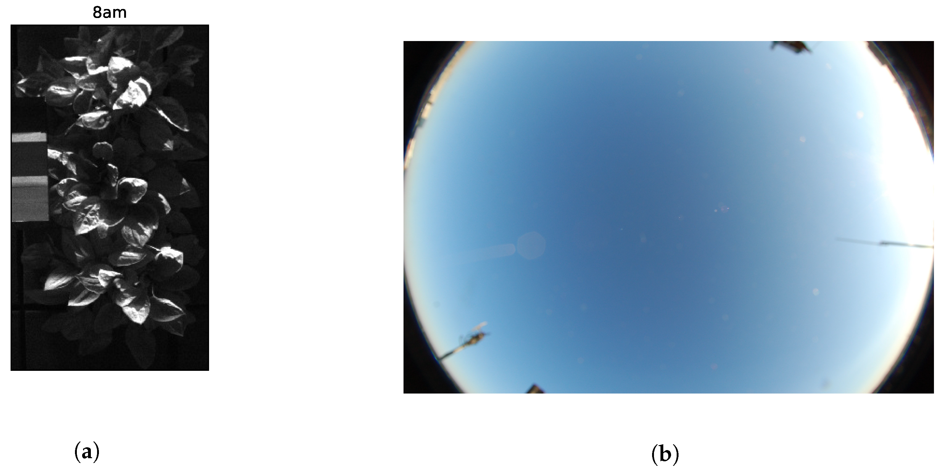
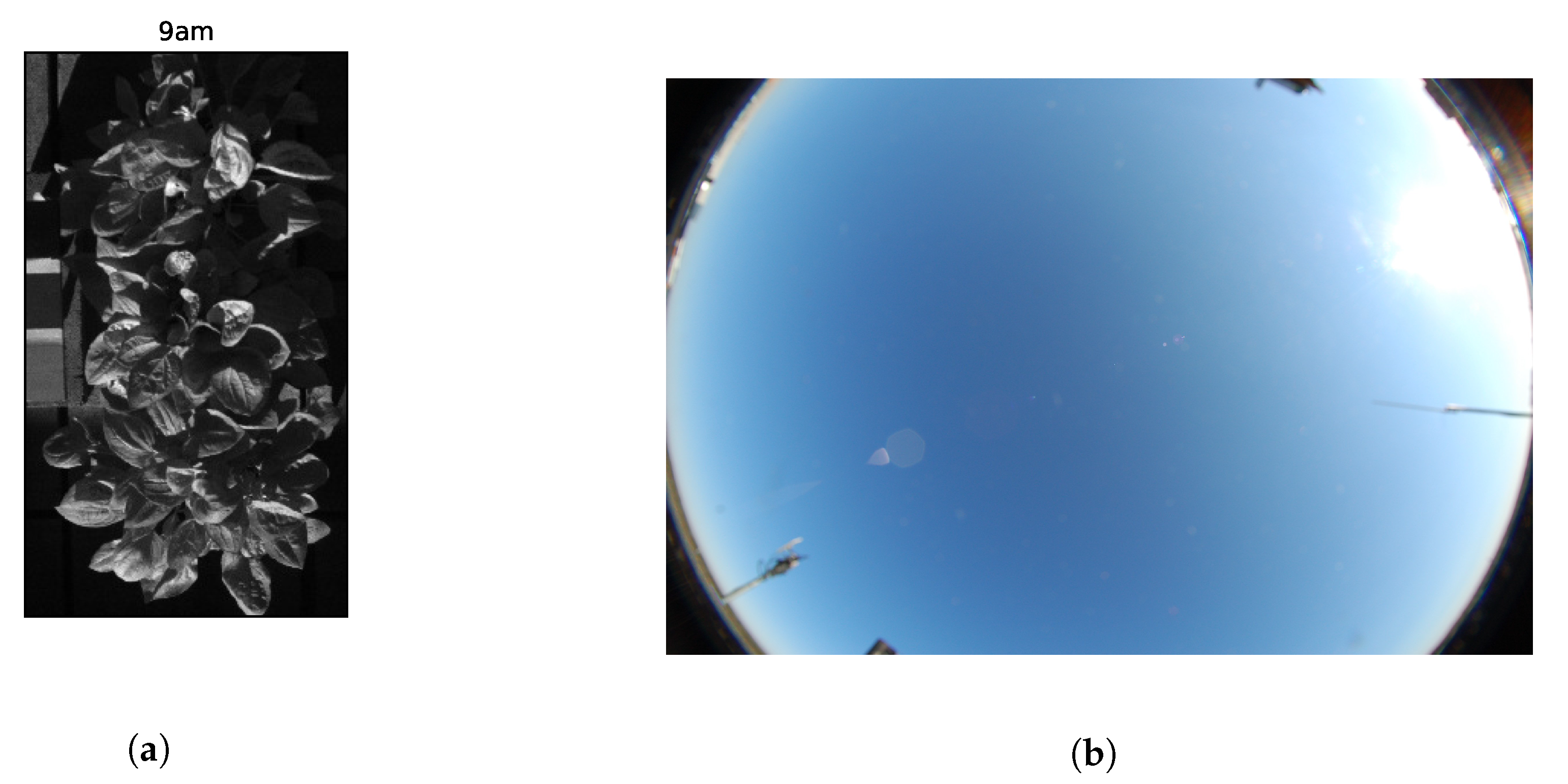
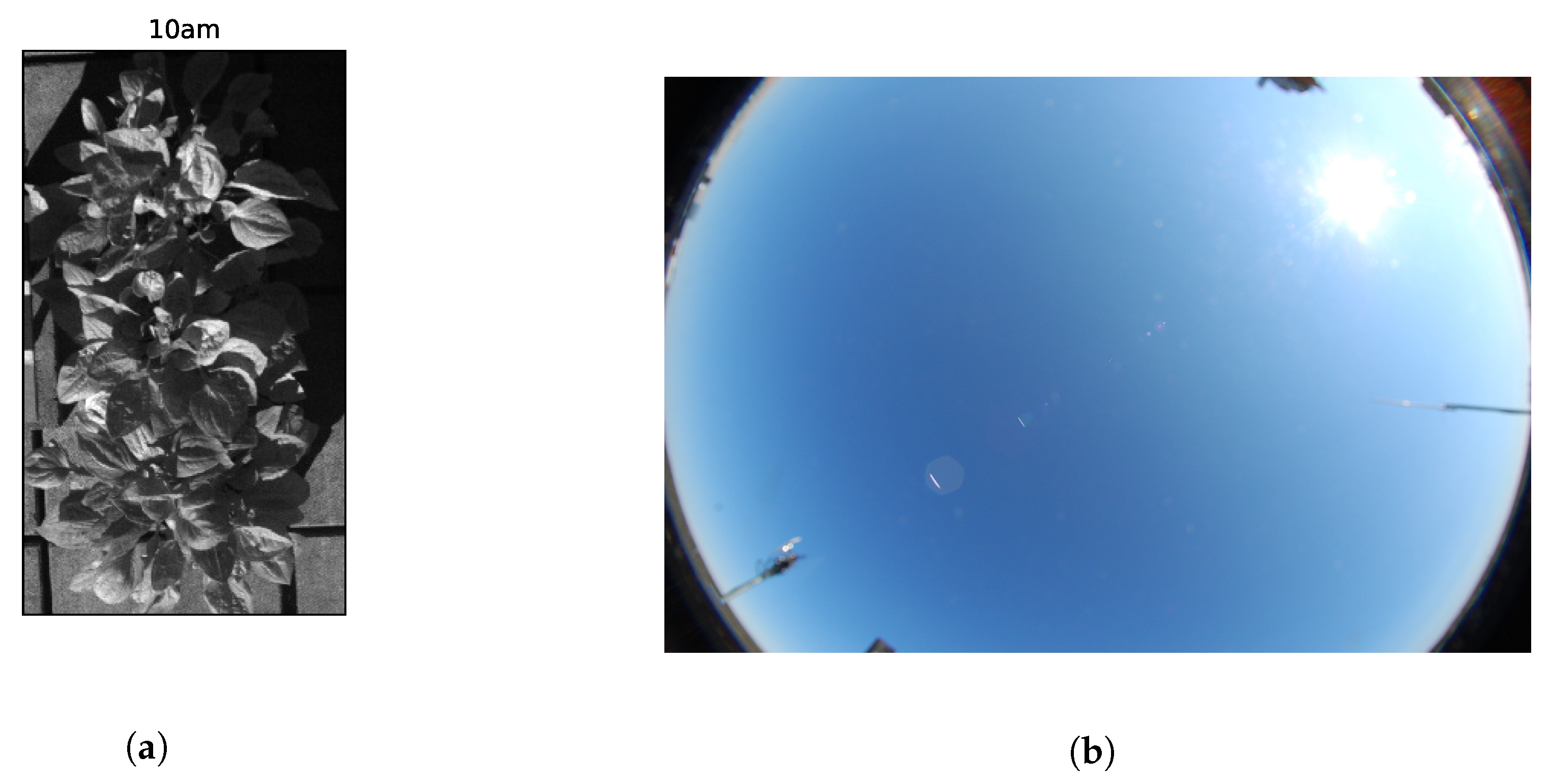
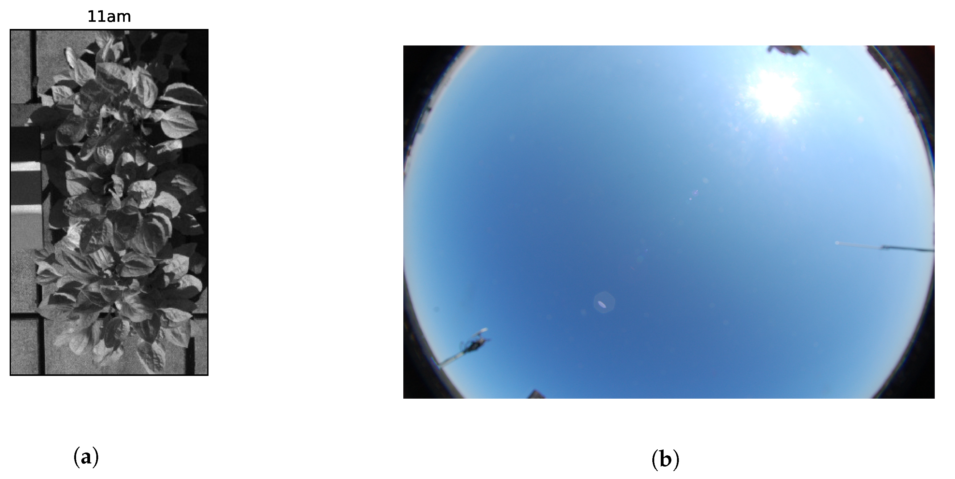
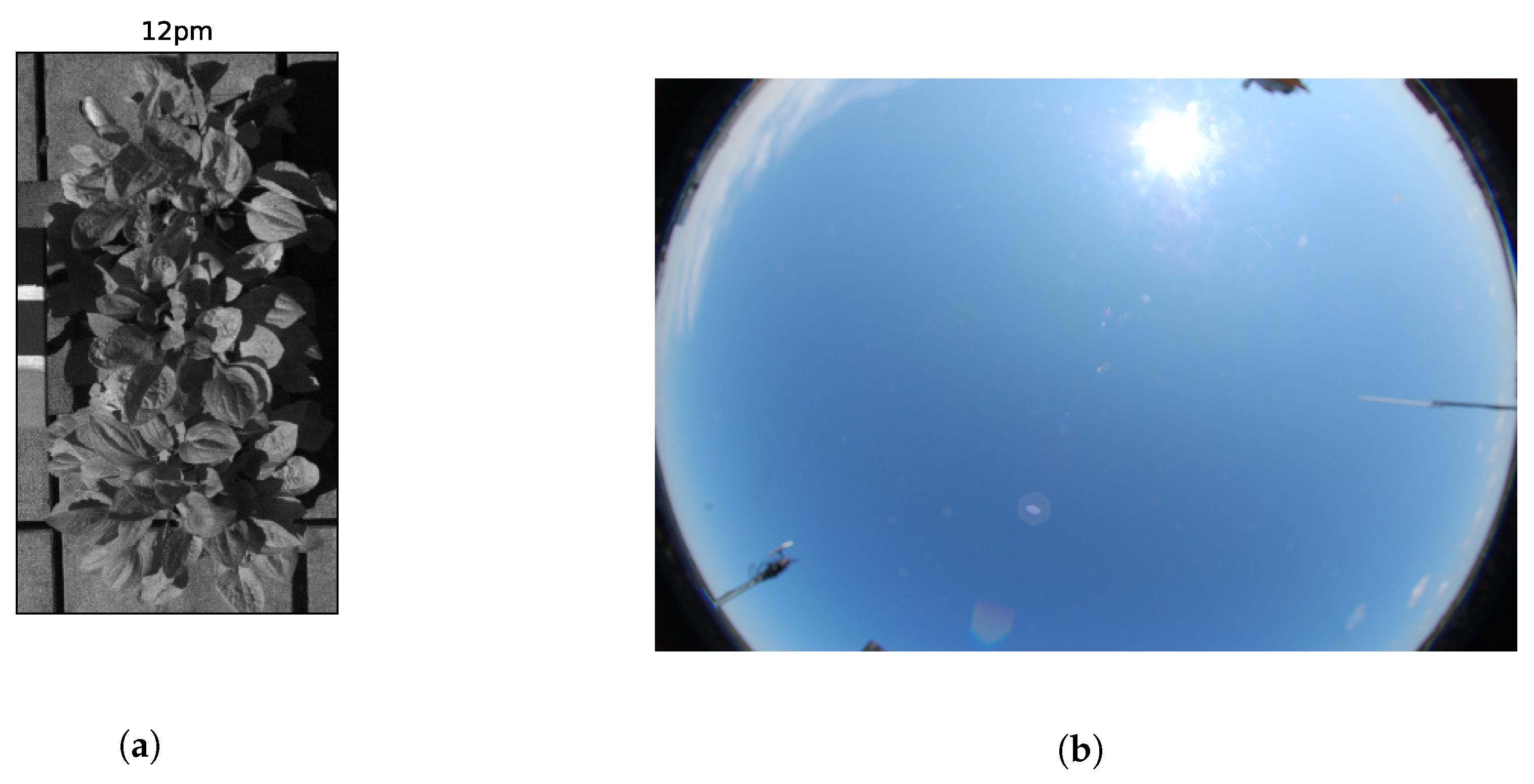
To showcase the affect of solar illumination, Figure 1, Figure 2, Figure 3, Figure 4 and Figure 5 displays the same scene captured at five various hours on a sunny day. These images were captured at the Rochester Institute of Technology Carlson Center for Imaging Science (43.0846 N, 77.6743 W). The difference in illumination and the shadow being cast is noticeable. These images showcase the variation in the imagery as the solar zenith angle decreases. These are important issues to consider because, while sUAS are exceptional for imaging agricultural fields, depending on the size of the field and how fast the sUAS is flying, the change in solar zenith angle during the data collection could impact the results. As demonstrated by Granzier, solar illumination changes based on time of day, season, and weather conditions [13].
2.2. Small Unmanned Aircraft System (sUAS)
Since the inception of precision agriculture, significant advancements have been made in both sensor technology and the platforms that carry these sensors [14]. With the development of sUAS, the capability of capturing high spatial resolution imagery at any moment in time has been achieved. These sUAS have become increasingly popular among both researchers as well as commercial businesses due to their relatively low initial start-up cost, straight forward implementation, and easy maintenance. They also provide users with long flight durations, mission safety and the ability to repeat the same flight pattern [14]. Limitations do exist for sUAS users, such as a maximum flying altitude of 122 m (in the United States) above the ground [15], and a limited battery life. On the other hand, it is possible to apply for waivers to fly over 122 m if required.
Various kinds of sensors have been utilized for precision agriculture. These sensors include, but are not limited to: multispectral, hyperspectral, LiDAR, short-wave infrared and long-wave infrared [16]. All of these sensors provide a unique look into the plants and provide different analytics on their health. For the purposes of this study, the MicaSense RedEdge-3 (MicaSense, Seattle, WA, USA), a field portable spectrometer—ASD Field Spec (Analytik Ltd., Cambridge, UK), and a high resolution handheld field portable spectroradiometer—SVC HR-1024i (Spectra Vista Corporation, Poughkeepsie, NY, USA), were used.
2.3. Multispectral Sensing
The MicaSense RedEdge-3 is a multispectral sensor that captures five channels simultaneously. It can capture as fast as one image per second with a 47.2 field of view (FOV). The sensor can be run in Auto capture or Manual mode. Auto capture mode sets gain and integration time for each channel separately based on the scene being imaged, while Manual mode allows the user to select these parameters. In addition, the RedEdge-3 comes with a downwelling light sensor (DLS) which measures the illumination (downwelling light) of the scene when each image is captured. The bands of the RedEdge-3 camera and their respective Full Width Half Max (FWHM) are listed in Table 1.
2.4. Conversion to Radiance
Utilizing MicaSense’s Radiometric Calibration Model, the raw digital count imagery can be converted into absolute spectral radiance [W/m/sr/nm]. This model addresses the vignette/row-gradient issues that exist in the raw images and then converts digital counts into radiance. The conversion process is demonstrated in both: [17], and [18].
2.5. Conversion to Reflectance
Converting raw digital counts to reflectance is a very important task in the field of remote sensing as it allows for different sets of imagery (or data) to be compared against one another. Without converting to reflectance, factors such as the illumination, integration time, and gain settings can drastically affect results. Two different methods will be used in this paper for reflectance conversion: Empirical Line Method and At-Altitude Radiance Ratio.
2.5.1. Empirical Line Method (ELM)
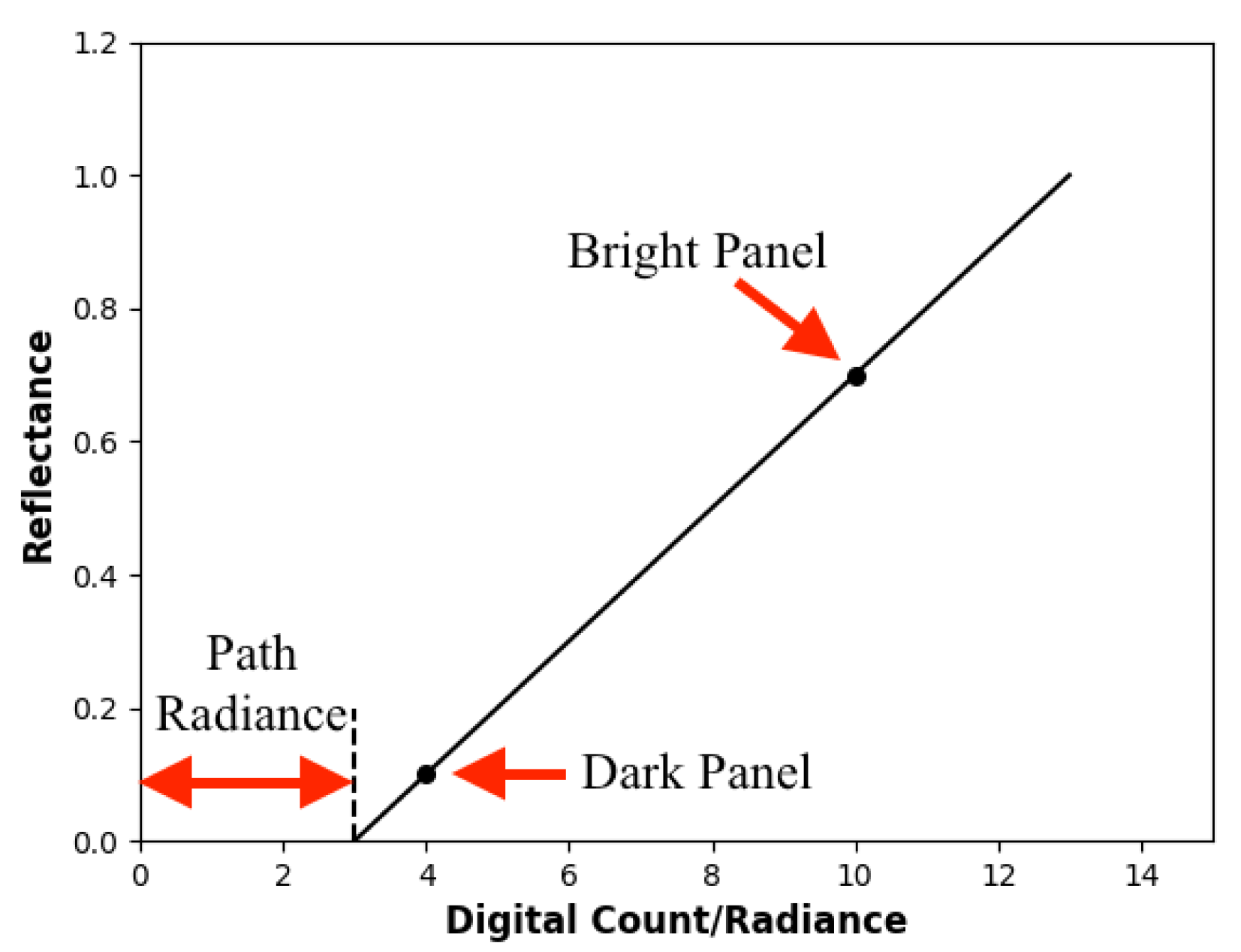
Empirical Line Method (ELM) is one the most well known techniques for converting either digital count or radiance imagery into reflectance imagery. The two variations of ELM that are used in this study are 2-Point ELM, and 1-Point ELM, although more can be used [19]. 2-Point ELM utilizes two reflectance conversion panels, a bright and a dark panel, to derive a conversion into reflectance, while 1-Point ELM only uses the bright panel and the origin (Radiance = 0, ). In addition, these reflectance conversion panels need to be measured at the time of data collection, so their reflectance values can be used to compute a best fit line. Since its inception, ELM has been used for a multitude of applications [20,21,22,23,24]. An example computation of ELM can be seen in Figure 6 and Equation (1).
where, is the reflectance factor, is the slope, is the band effective spectral radiance, is the bias, and i denotes the spectral band number. By using the computed slope and bias, the rest of the pixels in that image can be converted into reflectance.
2.5.2. At-Altitude Radiance Ratio (AARR)
One of the newest methods of reflectance correction, At-Altitude Radiance Ratio (AARR), was tested in-depth by Mamaghani et al. in 2018 [25]. This technique utilizes a downwelling light sensor (DLS) to convert radiance images into reflectance. This means that no reflectance conversion panels are required for the AARR technique. While AARR saves sUAS users significant time in the field (no need to deploy panels, record their spectra, etc.), and saves time in processing the data (locating the panels, applying ELM, etc.), the overall error was higher than ELM. After studying six targets from four altitudes and under three various weather conditions with a MicaSense RedEdge-3 sensor, AARR, 1-Point ELM, and 2-Point ELM produced −0.0244%, −0.0028%, −0.0050% average band effective reflectance factor errors respectively. This study also demonstrated that atmospheric effects (degradation in transmission and path radiance) are negligible up to 122 m, because 1-Point and 2-Point ELM produced similar overall band effective reflectance factor errors and standard deviations [25].
2.6. Reflectance Variation Importance
While AARR does not strictly outperform ELM, its performance is close enough to pose a new question: How accurate does the reflectance imagery have to be? Moreover, is the error that is produced when converting from digital count to reflectance overshadowed by other factors, mainly the inherent reflectance variability of the target in question? For example, if the variability in vegetation reflectance is lower than the error produced in the reflectance imagery, it is up to the sUAS user whether or not they would prefer to save time (AARR) or produce more accurate imagery (ELM). On the other hand, if the variability of vegetation is shown to be higher than the error produced during the conversion to reflectance, then utilizing a technique such as AARR is recommended because it saves the sUAS ground crew time in the field, less crew members are needed, and saves time during the data processing portion.
2.7. Normalized Difference Vegetation Index (NDVI)
Once the images have been converted to reflectance, vegetation health indices can be applied. Normalized Difference Vegetation Index (NDVI) is a metric that has been used to determine if a remotely sensed image contains healthy vegetation. By using the near-infrared and red channels, NDVI can be computed using Equation (2) [26,27].
NIR and Red bands are utilized because healthy vegetation (healthy chlorophyll) reflects more light in the NIR and green regions and absorbs more red light. With this in mind, NDVI values range between −1 (no or stressed vegetation), and 1 (very healthy vegetation). Some of the benefits of using NDVI are its stability over time as well as the fact that it is not very susceptible to noise [28]. Computation of NDVI can also be accomplished using other band combinations [29]. But, these combinations are not as frequently used as the NIR and red bands. While this research investigates the impact of illumination conditions on plant reflectance, and to a certain extent NDVI, other variables such as precipitation and temperature have an effect as well [30].
3. Materials and Methods
Six coneflowers (Rudbeckia fulgida) were used for data collection. Collections occured on 22 September and 24 September 2018 under cloudy and sunny conditions respectively. Background effects and temperature measurements were not taken into consideration during data collection for either the ASD or MicaSense measurements. On each day, data was collected from three plants with the following methodology at the top of every hour between 08:00 a.m. and 12:00 p.m. EST:
- Capture sky image with Nikon Camera
- Collect first set of ground reference reflectance of conversion panels
- Collect 15 min of MicaSense RedEdge-3 Imagery ( 90 images captured between minutes 3 and 18 every hour)
- Collect second set of ground reference reflectance of conversion panels
- Collect reflectance from all three plant’s using an ASD FieldSpec at three various heights (15 cm, 30 cm and 60 cm)
3.1. Field Spectroradiometer and Leafclip Contact Probe Measurements
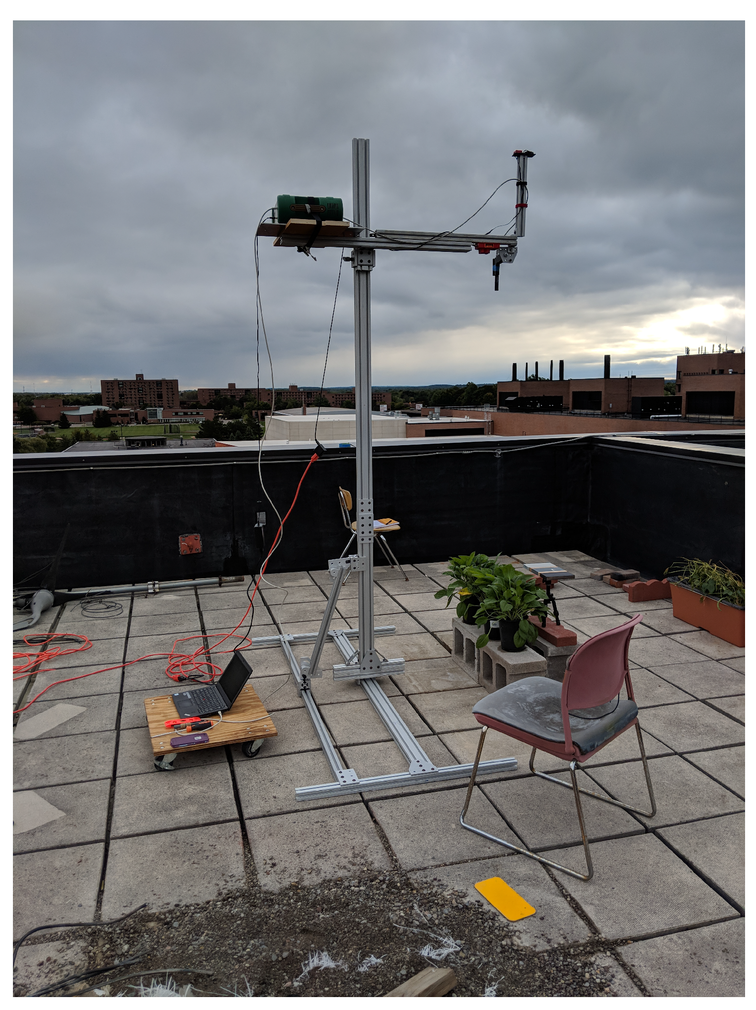
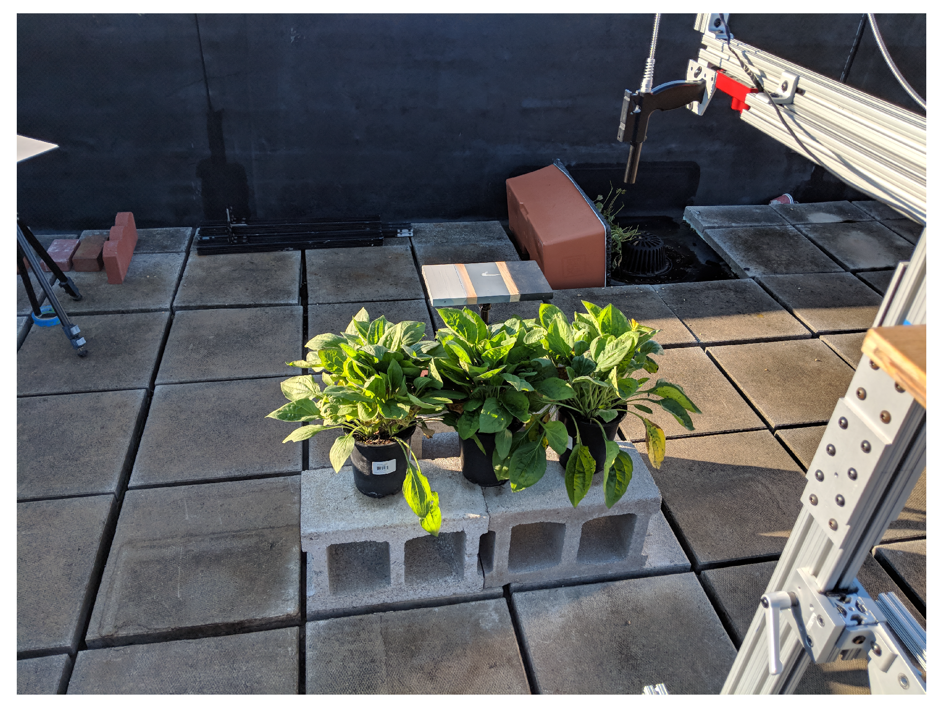
For every combination of time, height, and plant, five reflectance spectra files were recorded by the ASD. Each of these ASD reflectance spectra files were produced by averaging five measured spectra. Therefore, every combination of time, height and plant averaged 25 reflectance spectra. Furthermore, the heights of 15 cm, 30 cm, and 60 cm were selected because they produced 2 cm, 4 cm and 8 cm GSD with a 3-degree foreoptic. These GSDs correlate with a MicaSense RedEdge-3 capturing images at heights of 30.5 m, 61 m and 122 m. Finally, while measuring the reflectance of the plants, a before and after reference measurement was made of a 100% reflectance panel (that was horizontally level) to ensure the illumination was consistent throughout plant reflectance measurement. Figure 7 and Figure 8 show the collection setup and the plants measured. The setup picture was captured on the cloudy day (22 September) while the close up of the plants was captured on the sunny day (24 September 24).
After all of the MicaSense RedEdge-3 images and ASD measurements were completed, ten leaves on each of the plants were analyzed using a leafclip measurement tool that attached to the SVC HR-1024i spectroradiometer. This data collection was performed to measure the variability of reflectance on a single plant from a random selection of its leaves. Three locations on each leaf were selected at random and measured. These leafclip measurements were taken to measure the reflectance variability of vegetation in a controlled laboratory environment. Figure 9 displays the leafclip attached of the SVC spectroradiometer being used for measure an example leaf.
Once these spectra files were averaged, and standard deviations were computed, NDVI variability was able to be computed for all the measurement varieties. In addition, average and standard deviation spectra were computed for each plant using all leafclip contact probe measurements, along with their NDVI. This would provide a more accurate representation of the reflectance spectra of the Coneflower plants. In order to compute NDVI, the averaged reflectance spectra were integrated with the measured relative spectral response (RSR) functions of the MicaSense RedEdge-3. This produced band effective reflectance factors for all five bands of the RedEdge-3, which allowed for computation of NDVI.
3.2. Multispectral Sensor Measurements
After the RedEdge-3 images were converted into reflectance using all three methods (2-point ELM, 1-Point ELM, and AARR), a region of interest (ROI) over the plants was manually selected to use for analysis. All the pixels in the ROI were averaged together and utilized for statistical analysis of both the reflectance factor values and the NDVI of the plants. An example ROI is shown in Figure 10. Different ROIs were selected for each band of the sensor because the bands are not aligned.
3.3. DIRSIG5
Some of the measured reflectances were validated using DIRSIG5 software [31]. DIRSIG5 is a physically-based Monte Carlo path tracer—i.e., DIRSIG5 estimates the radiance incident upon a virtual detector array by tracing light transport paths randomly through a virtual scene, wherein triangles constitute virtual surfaces, which are characterized by energy-conserving light scattering models. Furthermore, DIRSIG5 is specifically designed to simulate multispectral (as well as hyperspectral) Earth-observing imagery, and accepts parameters such as geodetic location, absolute day and time, detector band positions and widths, and atmospheric characteristics.
To use DIRSIG5 for validation, a virtual scene was constructed at Rochester, NY (43.1566 N, 77.6088 W) on 24 September 2019, which is where and when the data were collected. The virtual scene consists of (1) A ground plane characterized by a spectrally-flat 5% reflectance chosen to mimic asphalt, (2) A pair of calibration panels characterized by field-measured reflectances of the actual calibration panels used in the collect, and, (3) A group of three procedurally-generated, ad hoc broadleaf plants characterized by field-measured leaf-level reflectances of the actual plants used in the collect.
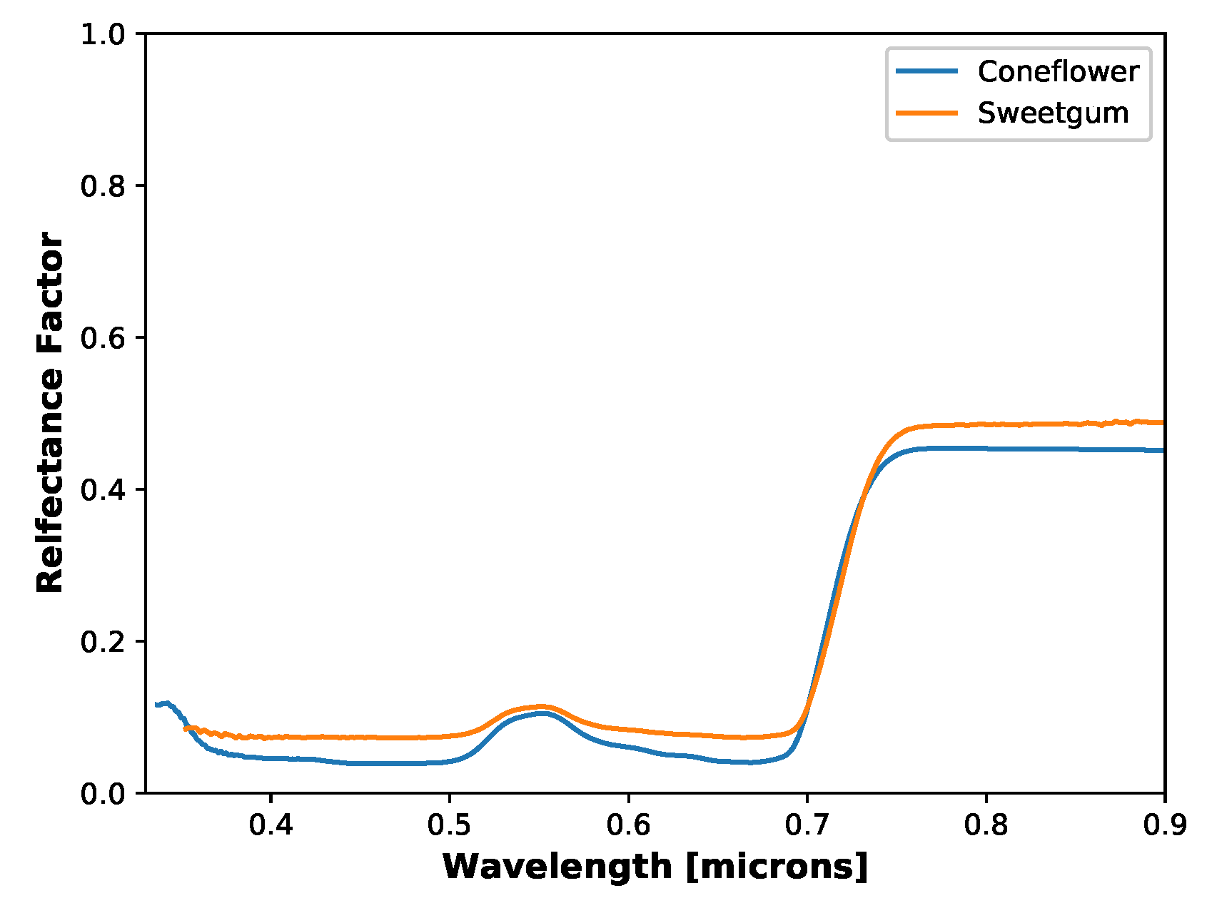
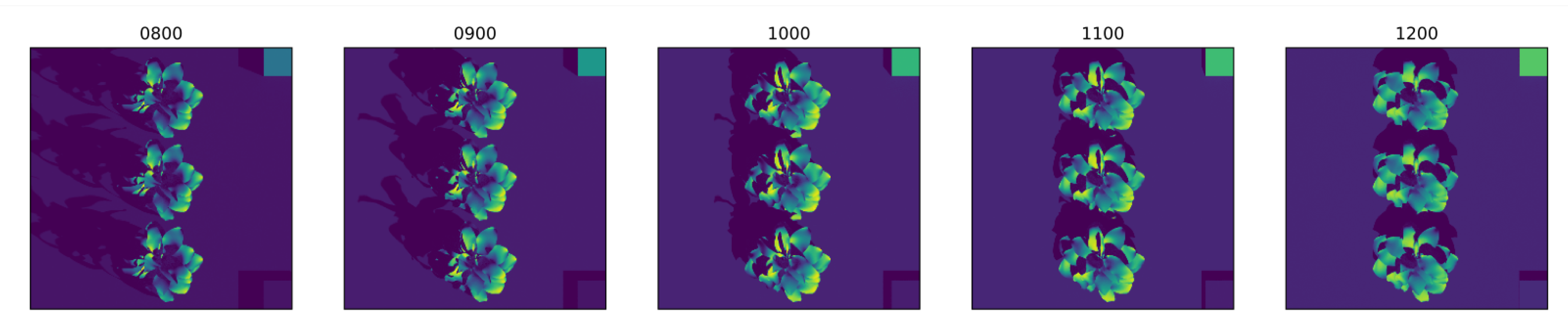
For simplicity, all surfaces use a Lambertian reflection model. However, to account for the significant increase in transmission by vegetation in the infrared, plant surfaces also use a Lambertian transmission model, whereby we attribute plant surfaces with a representative transmittance spectrum. Specifically, we attribute the transmittance of a Sweetgum leaf, which has a very similar reflectance to the leaf reflectances measured (Figure 11). The virtual detector array features five bands, corresponding to those of the Micasense imager. Using a mid-latitude summer atmospheric profile with no cloud cover, images were simulated at 08:00 a.m., 09:00 a.m., 10:00 a.m., 11:00 a.m., and 12:00 p.m. Figure 12 displays the scaled NIR bands of the DIRSIG images.
4. Results and Discussion
4.1. Field Spectroradiometer
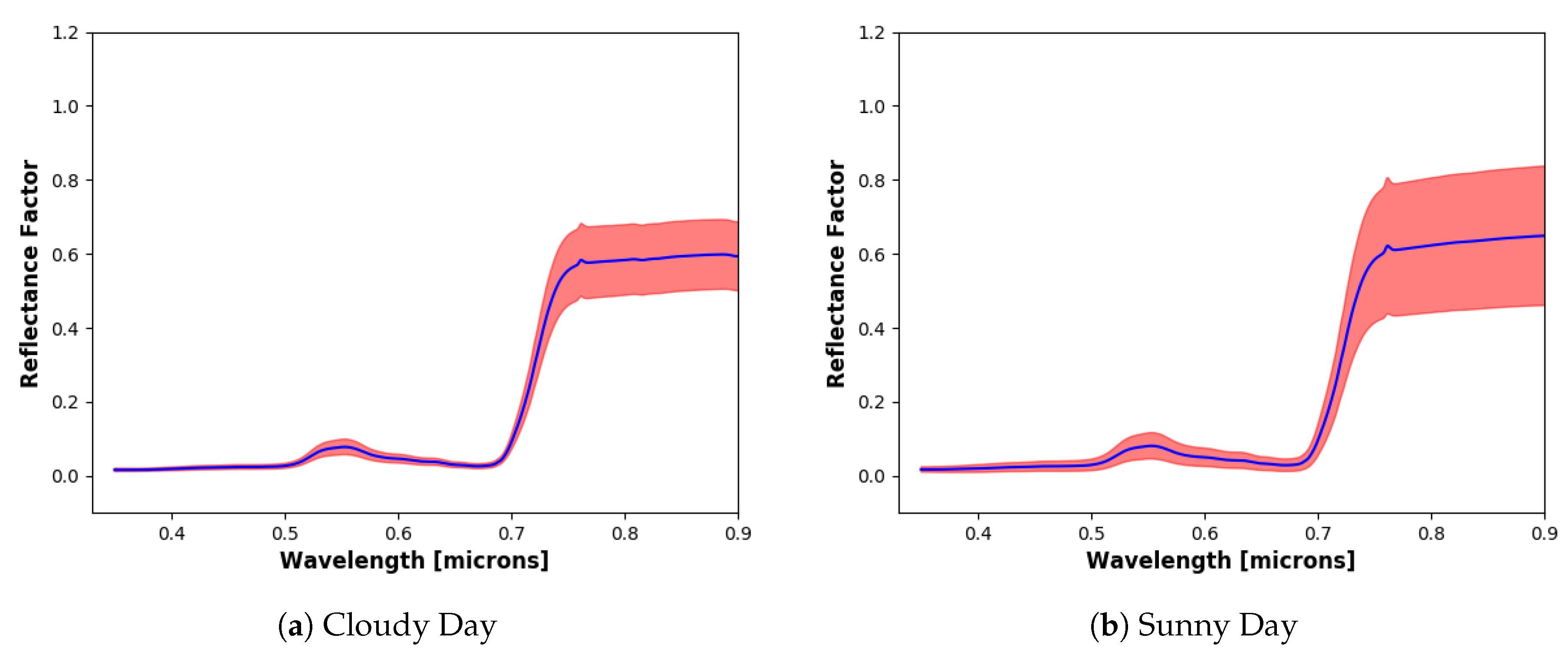
Figure 13 shows the average and standard deviation of the reflectance spectra measured on the cloudy and sunny days using the ASD. These results were computed by averaging over all three plants, all three heights, and all five hours on their respective days. Overall, the average reflectance spectra on both the cloudy and sunny days were very similar, as shown by the blue spectra in the Figures below. The significance of these results is the standard deviation of the measurements. As seen in the plots, the variability is very high in the infrared region of the spectrum (700 nm and higher). This is significant because many vegetation health indices use reflectance values from the infrared region, thus it is difficult to accurately measure the health of vegetation. Using the results in Figure 13, the computed NDVI is: 0.912 ± 0.026 on the cloudy day, and 0.905 ± 0.257 on the sunny day. While NDVI ranges between −1 and 1, some of the sunny day results would fall above 1. This is possible because of the varying leaf geometries that exist in the scene. The measured leaves that are angled directly at the sun will produce higher reflectance spectra curves, because the reference panel measured was horizontally level. In addition, some of the darker regions of the canopy (shadowed regions) will have a lower measured radiance than the reflectance conversion panels. This could produce negative reflectances in the Red band, which would produce NDVI values above 1.0. As stated before, the average NDVI computed using both data sets produce similar values, but the standard deviation is ten times higher for the sunny day. The two changing factors during these data collections were: the illumination (sun angle/time of day), and the orientation of the leaves. While the orientation of the leaves could change by gusts of wind, there was no way to measure or account for any change in orientation. However, the illumination was changing consistently as the time of day progresses, which creates the noticeably higher standard deviation.
Band effective reflectance factors were computed from the average ASD reflectances for every combination (Figure 14 and Figure 15).
NDVI was computed for every plant, time and GSD combination. NDVI were computed using the band effective reflectance factors from the ASD measurements shown above (Figure 16 and Figure 17). ASD measurements were not made for the Plant 2 at 12 p.m. because the cloud cover had passed.
NDVI results shown in Figure 16 and Figure 17 were expected, and there are a few ways to analyze the results. The first variable to analyze is the weather. The cloudy forecast produced a small NDVI variability regardless of which plant, GSD, or time of day was measured. The small decrease in NDVI that is seen as time progressed could be attributed to the orientation of the leaves when the data was collected, or because of the increase in illumination. While that sounds counter-intuitive, solar illumination still reaches the ground on a cloudy day, and if the cloud cover is consistent (uniform), the light travels through less clouds when it is directly overhead. This is the difference between direct illumination (direct sunlight), and diffuse illumination (sunlight scattered off atmospheric particles) [32]. This will produce a higher illumination near noon. For sunny conditions, the NDVI variability is more noticeable, specifically in in Plants 4 and 6. As the GSD changed, the NDVI changed. This is expected because sunny days produce shadows which can cover various leaves of the plant by self-shadowing (from other leaves). Therefore, higher GSDs cover more pixels on the plant, which could include more or less shadowed areas on the plant which will produce different NDVI values.
Two of the other variables that were tested in this experiment were the GSDs and time of day. The data collected on both the cloudy and sunny day showed no pattern with GSD. While the NDVI measured did change as the GSD was increased, there was no obvious correlation between NDVI and GSD. As previous stated, this is probably because the higher GSDs either measured more or less shadowed leaves, and without knowing the exactly percentage of shadowed coverage, there is no way to draw a correlation between NDVI and GSD. A one-way ANOVA test was used to determine if there was any significance across GSD. It was shown that for all plants, and times of day, the GSD produced statistically significant difference in NDVI (p < 0.001).
Overtime, the cloudy day displays a small decrease in NDVI as the day progressed. It is entirely possible that this small increase in illumination that occurs on cloudy days as the sun rises caused a small increase the reflectance measured in the Red and/or NIR channel, which could cause a slight decrease in the computed NDVI. On the other hand, the NDVI shows more scattering on the sunny day along the time variable. As the day progressed and the sun rose in the sky, the illumination and the cast shadows change on the plants, which alters the radiance being seen at the sensor. To further demonstrate the scattering, R values were computed across the time of day variable, and are displayed in Table 2. These values showed little to no correlation between time of day and NDVI, but did show higher correlations on the cloudy day, than the sunny day.
4.2. Leafclip Contact Probe
Figure 18 displays the average spectra and the respective standard deviations for all six plants. These leafclip spectra were captured by measuring three various locations from ten various leaves on each plant (30 measurements per plant).
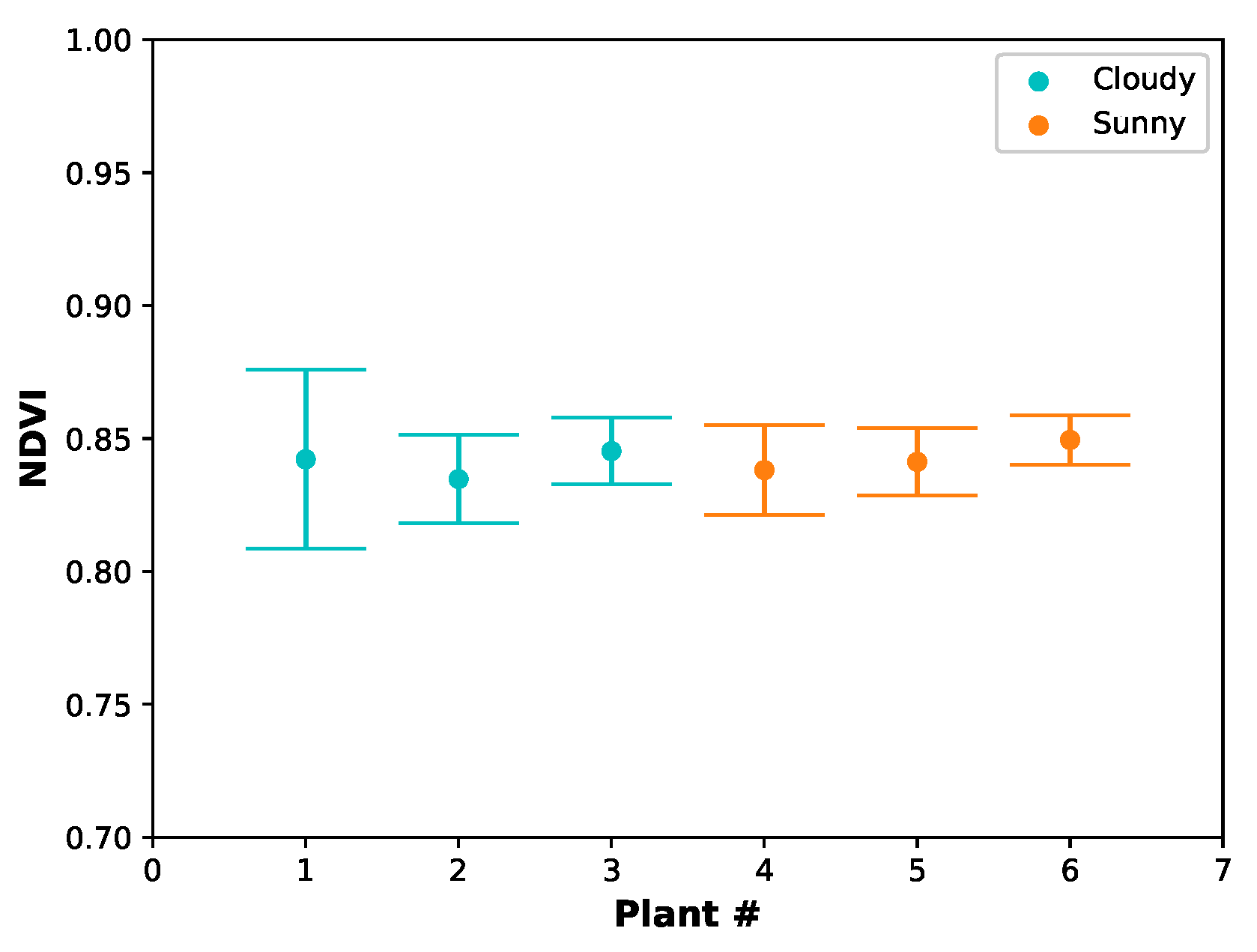
The plants produced nearly identical average reflectance spectra, and very similar standard deviations. This suggests that all the variations that were seen in the band effective reflectance factors from the ASD and MicaSense data were produced as a result of the conditions the plants were under (i.e., the illumination conditions). NDVI was also computed for each of the six plants (Figure 19). As expected, the average and standard deviations of the NDVI across all six plants did not vary significantly from one another. This was because the plant’s measured reflectance spectra produced very similar morphologies and reflectance values to each other, even though the spectra were measured from random locations on randomly selected leaves. In other words, the plants exhibited the same health index from randomly sampled selections. To showcase this, a one-way ANOVA test was performed on the computed NDVI values, which produced a p-value of 0.018. This result signifies that there is no statistically significant difference in the NDVI of leaves. The second takeaway from these results, is the standard deviation of the NDVI values, which ranged from 0.0095 to 0.0339. The highest standard deviation, Plant 1 (0.0339), is due to the higher variation at the red wavelength (∼668 nm) Plants 2 through 6 had less variation at that band, which is seen by the variation in the NDVI plots.
4.3. DIRSIG
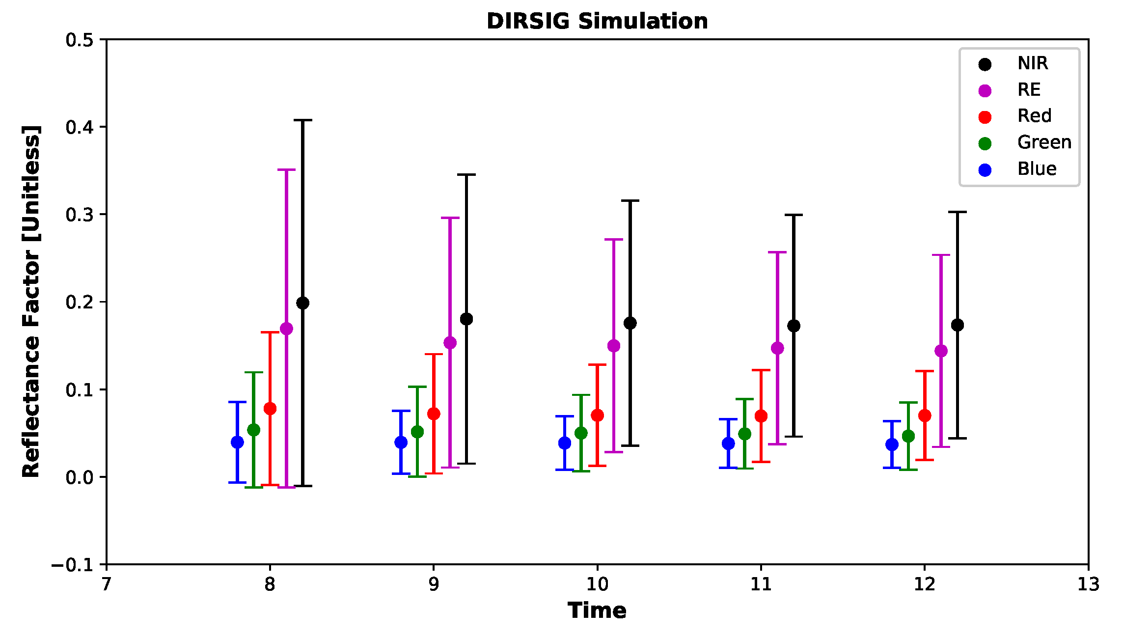
DIRSIG simulations also demonstrated this phenomenon as can be seen in Figure 20. The overall reflectance of the plants dropped as the solar zenith angle decreased. As can be seen by comparing Figure 20 with any of the scatter plots with error bars in Figure 21, the simulated DIRSIG band effective reflectance factors do not reproduce the MicaSense reflectance factors. This has been a difficult problem to investigate because of the number of variables affecting the simulation. Coneflowers (Rudbeckia fulgida) have a specific leaf structure and composition. While the virtual plants used in the DIRSIG simulation were generated to have the same shape and orientation, as well as the same representative reflectance and transmittance spectra as the Coneflowers used in the experiment, the specific scattering properties of the leaves were not taken into account. By default, we attributed Lambertian (constant) reflection and transmission properties to the leaves in the DIRSIG simulation. In reality, the leaves are certainly not perfectly Lambertian surfaces, and may exhibit scattering phenomena such as the Fresnel effect, whereby reflectivity increases as incident angle increases. As the effective reflectance factors are highly variable, and are in fact sensitive to leaf geometry as well as leaf scattering properties, we only expect the DIRSIG simulation to reproduce the MicaSense reflectance factors once a proper model of bidirectional leaf scattering properties is introduced.
4.4. Multispectral Sensor
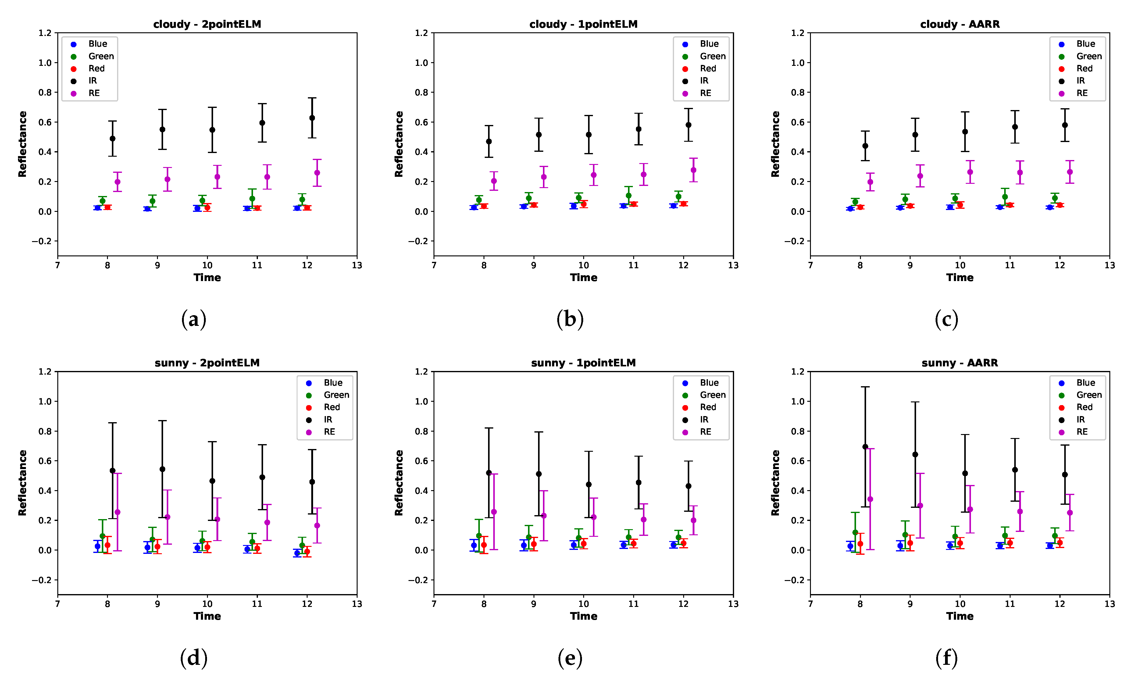
Figure 21 displays the average and standard deviation of the MicaSense reflectance imagery for all five hours, all three conversion techniques, and both days. Each average and standard deviation was computed from all of captured MicaSense images at that particular hour (90 images per hour).
There are a few interesting trends that can be seen in these MicaSense reflectance results. The first trend that can be seen is the increase in average reflectance on the cloudy day, as demonstrated by the R values seen in Table 3. The increase in average reflectance on the cloudy day is expected because as the solar zenith angle decreases, the light from the sun travels through less clouds (assuming a consistent cover). This increased the amount of illumination that reached the plants which increased the measured reflectance values.
The second trend is the higher standard deviation on the sunny day reflectances, as well as the overall decrease in reflectance overtime. The higher standard deviations are produced because the sunny day contains shadows which significantly vary the reflectance values of the scene. Shadowed leaf pixels will produce lower reflectance values than the illuminated leaf pixels in every band. While cloudy days also contain some faint shadows, they did not effect the standard deviations across time. In addition, there is a decrease in the overall reflectance in each band as the solar zenith angle decreases. This is because the self-shadowing of the plants increase as the sun rises (Figure 12), which decreases the overall measured reflectance in each band. The decrease in reflectance overtime is also showcased by the large R values seen in Table 3 as well as the values shown in Table 4.
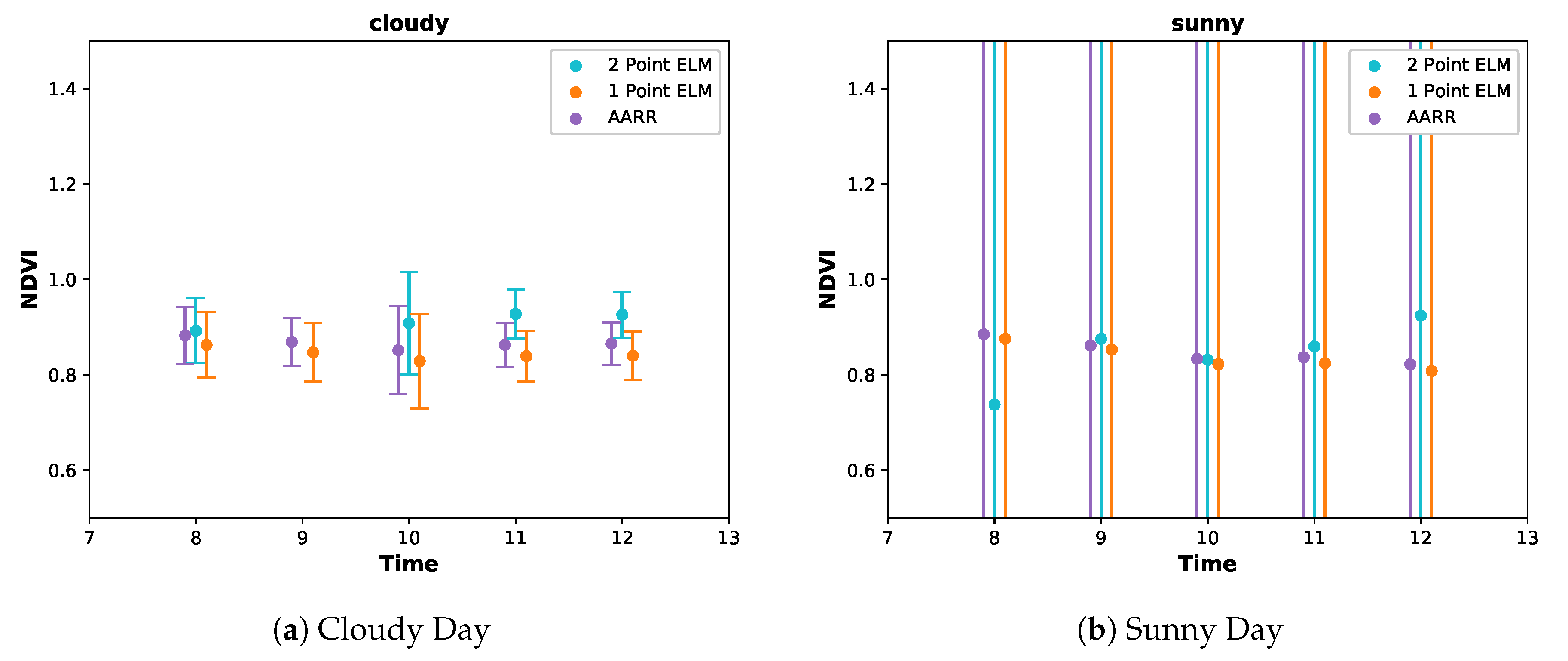
NDVI was also computed using the band effective reflectance factor results from the MicaSense data. The NDVI measured from the ROI of the plants can be seen below in Figure 22. These results again showcased the same trends. Significantly higher standard deviations were witnessed on the sunny day due to the self-shadowing of the plants. The NDVIs computed for the sunny day (Figure 22 (b)) had to be capped because the variability in both the Red and NIR channels produced negative or in some cases, higher than 1.0 reflectance factor values.
In the early years of remote sensing, when satellites and manned aircrafts were used, it was always desired to collect data on sunny and clear days. For satellites, this is obvious, because clouds would cover the targets that were being imaged. As for manned aircrafts, the illumination was desired for high signal to noise ratios (SNR). This way of thinking continued through to sUAS platforms as well. However, this study reached the opposite conclusion. Because sensors produce better resolution imagery, and sUAS can be flown closer to the targets of interest, SNR is not as big of a concern as the variability in the data. The data collected shows that cloudy days around noon are the best time for collection of sUAS imagery because of the smaller variation produced in the results. Without clouds, shadows impact results on a greater scale for sUAS imagery (because of the higher resolution/smaller GSDs). Noon can be seen as the optimal time because, in the event that the clouds are not perfectly uniform, a solar zenith angle close to 0 would produce the lowest variation while providing a good SNR.
5. Future Work
5.1. Data Recollection
To further investigate, a subsection of this study could be accomplished which would allow the data being collected to be more precise. When the ASD rig was shifted horizontally from plant to plant, and also raised to capture various GSDs, the collection team did their best to ensure the ASD rig was placed back into the exact same spot. It was impossible to place the ASD rig back into the previous position, therefore, ASD measurements could have been made from slightly different locations above the plants, which would result in improper comparison of reflectances as well as NDVI measurements. Recollecting a subsection of the data from this experiment would ensure that the ASD never moves, and the same part of the plant canopy is measured. For example, only measuring a single plant, from one height, at various times. This would reduce the human error component for the ASD data collection and ensure that the same area of the plant canopy (leaves) is measured every time. Second, by recording the temperature during data collection, potential trends between the reflectances or NDVI and temperature could have also been investigated. Third, if data recollection was performed, using more plants would be highly recommended. By filling the entire MicaSense RedEdge-3’s field of view with plants, albedo effects from the background would be removed, and this would better simulate a farmer’s field. Finally, a smaller ROI could have been used to compute the reflectance factors from the RedEdge-3 imagery. For example, using a 20 × 20, 40 × 40, or 80 × 80 ROI for a MicaSense RedEdge-3 sensor at 1.5 m would correspond to 2, 4, and 8 cm GSD respectively.
5.2. Entire Simulation Study
This entire study could also be performed using simulations produced by software like DIRSIG. By collecting lots of leaf reflectances, and even the Bidirectional Reflectance Distribution Function (BRDF) of the coneflower leaves (using software such as PROSAIL), a more accurate representation of a coneflower plant could be simulated and tested across a multitude of variables: days, seasons, latitudes/longitudes, weather conditions, etc. Even the plant could be changed from coneflower to whatever vegetation the user wishes to study. This could provide agricultural scientists, and remote sensing practitioners with incredible insights into vegetation variability.
5.3. Reflectance Variability of Target X
While this study focuses on a particular plant, there are many other crops that could have been studied. Those other plants could have produced a different result simply because their leaf structure is vastly different than that of a coneflower. It is recommended to study the variability of one’s target of interest before making a decision on which calibration and reflectance conversion techniques to utilize. There is a possibility that some targets being studied have little to no variability.
6. Conclusions
This study investigated the variation in reflectance spectra of six coneflower (Rudbeckia fulgida) plants. These plants were measured using an ASD spectroradiometer under different forecasts (cloudy and sunny), at different times (08:00 a.m., 09:00 a.m., 10:00 a.m., 11:00 a.m. and 12:00 p.m.), and at different GSDs (2, 4 and 8 cm). The collected ASD spectra were compared against leafclip contact probe measurements, as well as MicaSense RedEdge-3 reflectance imagery. ASD results showed no correlation across times or GSDs (one-way ANOVA p < 0.001, and low R). The cloudy day produced less variation in both reflectance factor, and NDVI when compared to the sunny day. This was caused by the shadows that were present on the sunny day. Finally the leafclip spectra demonstrated the similarity in reflectance spectra and the health of all the coneflower plants used in the study one-way ANOVA p-value of 0.018. Ultimately, the results showcased in this study have shown the high variability in vegetation reflectance regardless of the time, forecast, GSD, or plants being measured. These variabilities are much higher than the reflectance factor errors produced by the AARR conversion technique. This indicates that AARR is accurate enough for the purposes of agricultural remote sensing. With this new insight, it is recommended to capture sUAS vegetation imagery on cloudy days, at 8 cm GSD (or larger), and as close to noon as possible. This setup will produce the lowest variability for the vegetation being measured as demonstrated by the ASD field spectrometer measurements, MicaSense RedEdge-3 images, and the DIRSIG simulated images. It is also recommended to do a similar study for any target the remote sensing practitioner is investigating. These other targets may not posses the same inherent reflectance variability.
Author Contributions
This manuscript represents a portion of the research conducted by B.M. in pursuit of his doctoral degree in Imaging Science at the Rochester Institute of Technology. B.M. was the primary author, conducted all of the experiments, performed all data curation, prepared the visualizations presented in this manuscript, and was responsible for the analyses carried out. M.G.S. designed and produced the DIRSIG simulations used in the comparative analyses and assisted in the writing of the manuscript. C.S. served as B.M.’s doctoral advisor, assisted in the experiment planning and conceptualization, guided the analyses conducted, and contributed to the authoring and editing of this manuscript.
Funding
This research received funding from the Office of the Vice President for Research at the Rochester Institute of Technology through the Signature Interdisciplinary Research Areas—Center for Unmanned Aircraft Systems Research program, the Director of the Chester F. Carlson Center for Imaging Science at the Rochester Institute of Technology, and the L3Harris Corporation under contract number 915388J titled “Infrastructure Monitoring Using Aerial Drone Imaging Systems”.
Conflicts of Interest
The authors declare no conflict of interest.
References
- Robertson, M.; Carberry, P.; Brennan, L. The Economic Benefits of Precision Agriculture: Case Studies from Australian Grain Farms. Crop Pasture Sci. 2007, 60, 2012. [Google Scholar]
- Stafford, J.V. Implementing Precision Agriculture in the 21st Century. J. Agric. Eng. Res. 2000, 76, 267–275. [Google Scholar] [CrossRef]
- Zhang, C.; Kovacs, J.M. The application of small unmanned aerial systems for precision agriculture: A review. Precis. Agric. 2012, 13, 693–712. [Google Scholar] [CrossRef]
- Moran, M.; Inoue, Y.; Barnes, E. Opportunities and limitations for image-based remote sensing in precision crop management. Remote Sens. Environ. 1997, 61, 319–346. [Google Scholar] [CrossRef]
- Yang, C.; Everitt, J.H.; Bradford, J.M. Comparison of QuickBird Satellite Imagery and Airborne Imagery for Mapping Grain Sorghum Yield Patterns. Precis. Agric. 2006, 7, 33–44. [Google Scholar] [CrossRef]
- McBratney, A.; Whelan, B.; Ancev, T.; Bouma, J. Future Directions of Precision Agriculture. Precis. Agric. 2005, 6, 7–23. [Google Scholar] [CrossRef]
- Bauer, M.E. Spectral inputs to crop identification and condition assessment. Proc. IEEE 1985, 73, 1071–1085. [Google Scholar] [CrossRef]
- Ollinger, S.V. Sources of variability in canopy reflectance and the convergent properties of plants. New Phytol. 2011, 189, 375–394. [Google Scholar] [CrossRef] [PubMed]
- Kollenkark, J.C.; Vanderbilt, V.C.; Daughtry, C.S.T.; Bauer, M.E. Influence of solar illumination angle on soybean canopy reflectance. Appl. Opt. 1982, 21, 1179–1184. [Google Scholar] [CrossRef] [PubMed]
- de Souza, E.G.; Scharf, P.C.; Sudduth, K.A. Sun position and cloud effects on reflectance and vegetation indices of corn. Agron. J. 2010, 102, 734–744. [Google Scholar] [CrossRef]
- Suits, G.H. The calculation of the directional reflectance of a vegetative canopy. Remote Sens. Environ. 1971, 2, 117–125. [Google Scholar] [CrossRef]
- Smith, J.; Berry, J.; Heimes, F. Signature Extension for Sun Angle; Colorado State University: Fort Collins, CO, USA, 1975; Volume 1. [Google Scholar]
- Granzier, J.J.; Valsecchi, M. Variations in daylight as a contextual cue for estimating season, time of day, and weather conditions. J. Vis. 2014, 14, 22. [Google Scholar] [CrossRef] [PubMed]
- Watts, A.; Ambrosia, V.; Hinkley, E.A. Unmanned Aircraft Systems in Remote Sensing and Scientific Research: Classification and Considerations of Use. Remote Sens. 2012, 4, 1671–1692. [Google Scholar] [CrossRef]
- Unmanned Aircraft Systems. Available online: https://www.faa.gov/uas/ (accessed on 6 October 2018).
- Mulla, D.J. Twenty five years of remote sensing in precision agriculture: Key advances and remaining knowledge gaps. Biosyst. Eng. 2013, 114, 358–371. [Google Scholar] [CrossRef]
- MicaSense Incorporated. Image Processing. Available online: https://github.com/micasense/imageprocessing (accessed on 13 December 2018).
- Mamaghani, B.; Salvaggio, C. Multispectral Sensor Calibration and Characterization for sUAS Remote Sensing. Sensors 2019, 19, 4453. [Google Scholar] [CrossRef] [PubMed]
- Padró, J.C.; Muñoz, F.J.; Ávila, L.; Pesquer, L.; Pons, X. Radiometric Correction of Landsat-8 and Sentinel-2A Scenes Using Drone Imagery in Synergy with Field Spectroradiometry. Remote Sens. 2018, 10, 1687. [Google Scholar] [CrossRef]
- Karpouzli, E.; Malthus, T. The empirical line method for the atmospheric correction of IKONOS imagery. Int. J. Remote Sens. 2003, 24, 1143–1150. [Google Scholar] [CrossRef]
- Kruse, F.; Kierein-Young, K.; Boardman, J. Mineral mapping at Cuprite, Nevada with a 63-channel imaging spectrometer. Photogramm. Eng. Remote Sens. 1990, 56, 83–92. [Google Scholar]
- Laliberte, A.S.; Goforth, M.A.; Steele, C.M.; Rango, A. Multispectral remote sensing from unmanned aircraft: Image processing workflows and applications for rangeland environments. Remote Sens. 2011, 3, 2529–2551. [Google Scholar] [CrossRef]
- Moran, M.S.; Bryant, R.; Thome, K.; Ni, W.; Nouvellon, Y.; Gonzalez-Dugo, M.; Qi, J.; Clarke, T. A refined empirical line approach for reflectance factor retrieval from Landsat-5 TM and Landsat-7 ETM+. Remote Sens. Environ. 2001, 78, 71–82. [Google Scholar] [CrossRef]
- Smith, G.M.; Milton, E.J. The use of the empirical line method to calibrate remotely sensed data to reflectance. Int. J. Remote Sens. 1999, 20, 2653–2662. [Google Scholar] [CrossRef]
- Mamaghani, B.; Salvaggio, C. Comparative study of panel and panelless-based reflectance conversion techniques for agricultural remote sensing. arXiv 2019, arXiv:1910.03734. [Google Scholar]
- Rouse, J., Jr.; Haas, R.; Schell, J.; Deering, D. Monitoring vegetation systems in the Great Plains with ERTS. In NASA Goddard Space Flight Center 3d ERTS-1 Symposium, Proceedings of the Third Symposium on Significant Results Obtained from the First Earth, Washington, DC, USA, 10–14 December 1974; NASA: Washington, DC, USA, 1974. [Google Scholar]
- Doraiswamy, P.C.; Moulin, S.; Cook, P.W.; Stern, A. Crop Yield Assessment from Remote Sensing. Photogramm. Eng. Remote Sens. 2003, 69, 665–674. [Google Scholar] [CrossRef]
- Huete, A.; Didan, K.; Miura, T.; Rodriguez, E.; Gao, X.; Ferreira, L. Overview of the radiometric and biophysical performance of the MODIS vegetation indices. Remote Sens. Environ. 2002, 83, 195–213. [Google Scholar] [CrossRef]
- Thenkabail, P.S.; Lyon, J.G. Hyperspectral Remote Sensing of Vegetation; CRC Press: Boca Raton, FL, USA, 2011. [Google Scholar]
- Wang, J.; Rich, P.M.; Price, K.P. Temporal responses of NDVI to precipitation and temperature in the central Great Plains, USA. Int. J. Remote Sens. 2003, 24, 2345–2364. [Google Scholar] [CrossRef]
- Goodenough, A.A.; Brown, S.D. DIRSIG5: Next-Generation Remote Sensing Data and Image Simulation Framework. IEEE J. Sel. Top. Appl. Earth Obs. Remote Sens. 2017, 10, 4818–4833. [Google Scholar] [CrossRef]
- Padró, J.C.; Carabassa, V.; Balagué, J.; Brotons, L.; Alcañiz, J.M.; Pons, X. Monitoring opencast mine restorations using Unmanned Aerial System (UAS) imagery. Sci. Total Environ. 2019, 657, 1602–1614. [Google Scholar] [CrossRef]
Figure 1.
(a) NIR image captured by MicaSense RedEdge-3 of coneflower plants and (b) Sky at 8 a.m. on 24 September 2019. These images were captured at the Rochester Institute of Technology Carlson Center for Imaging Science (43.05′09.5″ N 77.40′39.6″ W).
Figure 1.
(a) NIR image captured by MicaSense RedEdge-3 of coneflower plants and (b) Sky at 8 a.m. on 24 September 2019. These images were captured at the Rochester Institute of Technology Carlson Center for Imaging Science (43.05′09.5″ N 77.40′39.6″ W).

Figure 2.
(a) NIR image captured by MicaSense RedEdge-3 of coneflower plants and (b) Sky at 9 a.m. on 24 September 2019. These images were captured at the Rochester Institute of Technology Carlson Center for Imaging Science (43.05′09.5″ N 77.40′39.6″ W).
Figure 2.
(a) NIR image captured by MicaSense RedEdge-3 of coneflower plants and (b) Sky at 9 a.m. on 24 September 2019. These images were captured at the Rochester Institute of Technology Carlson Center for Imaging Science (43.05′09.5″ N 77.40′39.6″ W).

Figure 3.
(a) NIR image captured by MicaSense RedEdge-3 of coneflower plants and (b) Sky at 10 a.m. on 24 September 2019. These images were captured at the Rochester Institute of Technology Carlson Center for Imaging Science (43.05′09.5″ N 77.40′39.6″ W).
Figure 3.
(a) NIR image captured by MicaSense RedEdge-3 of coneflower plants and (b) Sky at 10 a.m. on 24 September 2019. These images were captured at the Rochester Institute of Technology Carlson Center for Imaging Science (43.05′09.5″ N 77.40′39.6″ W).

Figure 4.
(a) NIR image captured by MicaSense RedEdge-3 of coneflower plants and (b) Sky at 11 a.m. on 24 September 2019. These images were captured at the Rochester Institute of Technology Carlson Center for Imaging Science (43.05′09.5″ N 77.40′39.6″ W).
Figure 4.
(a) NIR image captured by MicaSense RedEdge-3 of coneflower plants and (b) Sky at 11 a.m. on 24 September 2019. These images were captured at the Rochester Institute of Technology Carlson Center for Imaging Science (43.05′09.5″ N 77.40′39.6″ W).

Figure 5.
(a) NIR image captured by MicaSense RedEdge-3 of coneflower plants and (b) Sky at 12 p.m. on 24 September 2019. These images were captured at the Rochester Institute of Technology Carlson Center for Imaging Science (43.05′09.5″ N 77.40′39.6″ W).
Figure 5.
(a) NIR image captured by MicaSense RedEdge-3 of coneflower plants and (b) Sky at 12 p.m. on 24 September 2019. These images were captured at the Rochester Institute of Technology Carlson Center for Imaging Science (43.05′09.5″ N 77.40′39.6″ W).

Figure 6.
Example 2-Point Empirical Line Method best fit line. Bright and dark panel reflectance values measured in scene which allows for linear relationship between digital count/radiance and reflectance to be formed. Any offset from the origin is considered as path radiance.
Figure 6.
Example 2-Point Empirical Line Method best fit line. Bright and dark panel reflectance values measured in scene which allows for linear relationship between digital count/radiance and reflectance to be formed. Any offset from the origin is considered as path radiance.

Figure 7.
Setup used for data collection. MicaSense RedEdge-3 and ASD FieldSpec are attached on the arm of the rig. Rig was designed to move vertically as well as horizontally to allow for data collection for all three plants at all three heights. Laptop at base of rig was used to run the ASD. Image was taken on 22 September (cloudy day).

Figure 8.
Close up image of the Coneflower plants. ASD set at 15 cm (2 cm GSD) over Plant 6 (right most plant). Reflectance conversion panel can be seen behind the plants. Panel contains bright, medium grey, and dark sections. Image was taken on 24 September (sunny day).
Figure 8.
Close up image of the Coneflower plants. ASD set at 15 cm (2 cm GSD) over Plant 6 (right most plant). Reflectance conversion panel can be seen behind the plants. Panel contains bright, medium grey, and dark sections. Image was taken on 24 September (sunny day).

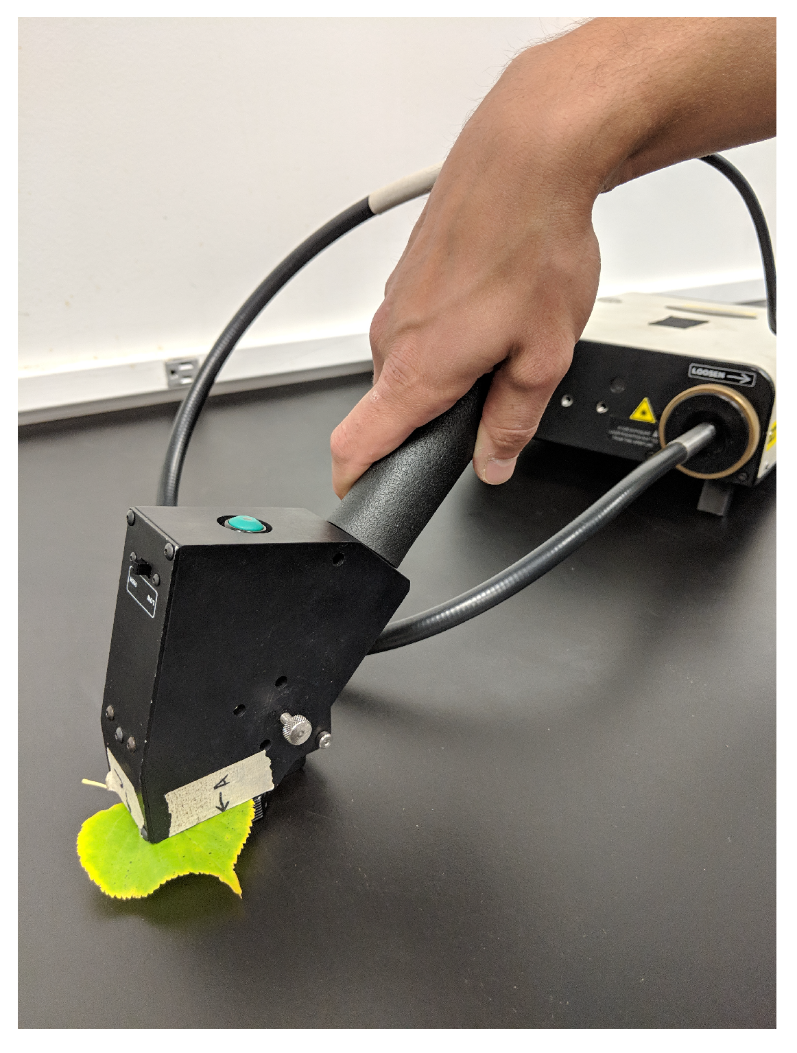
Figure 9.
Example leafclip measurement. SVC HR-1024i spectroradiometer is seen in the back. This example measurement image was staged after the collection. In reality, the leaves were measured while they were still attached to the plant.
Figure 9.
Example leafclip measurement. SVC HR-1024i spectroradiometer is seen in the back. This example measurement image was staged after the collection. In reality, the leaves were measured while they were still attached to the plant.

Figure 10.
Example region of interest selection from MicaSense (a) Blue (b) Green (c) Red (d) RedEdge and (e) NIR channel images. Reflectance conversion panel can be seen to the left of the plants. Image displayed was captured at 11 a.m. on 24 September 2018 (sunny day). Images captured at a height of 1.5 m, which translates to a frame size of 96 × 128 cm.

Figure 11.
Example Coneflower and Sweetgum leafclip contact probe reflectance measurements.

Figure 12.
DIRSIG simulations of sunny day. Images range from 08:00 a.m. to 12:00 p.m. Three coneflower plants were generated for the simulation. leafclip measurements (shown later) were utilized for the simulated plant reflectances. These images were converted into reflectance using 2-Point ELM. Bright panel in the top right corner, and the dark panel in bottom left corner were used for this conversion. Self-shadowing on the plants increases as the solar zenith angle decreases, which ultimately lowers the measured reflectances.

Figure 13.
Average ASD results from (a) cloudy day, and (b) sunny day. Reflectance spectra were computed by averaging all spectra collected by the ASD on the particular day (three plants, three heights, five times). Average reflectance spectra shown in blue, while one standard deviation is displayed as the red region. Average reflectance values similar across both days, but standard deviation was much higher on sunny day.

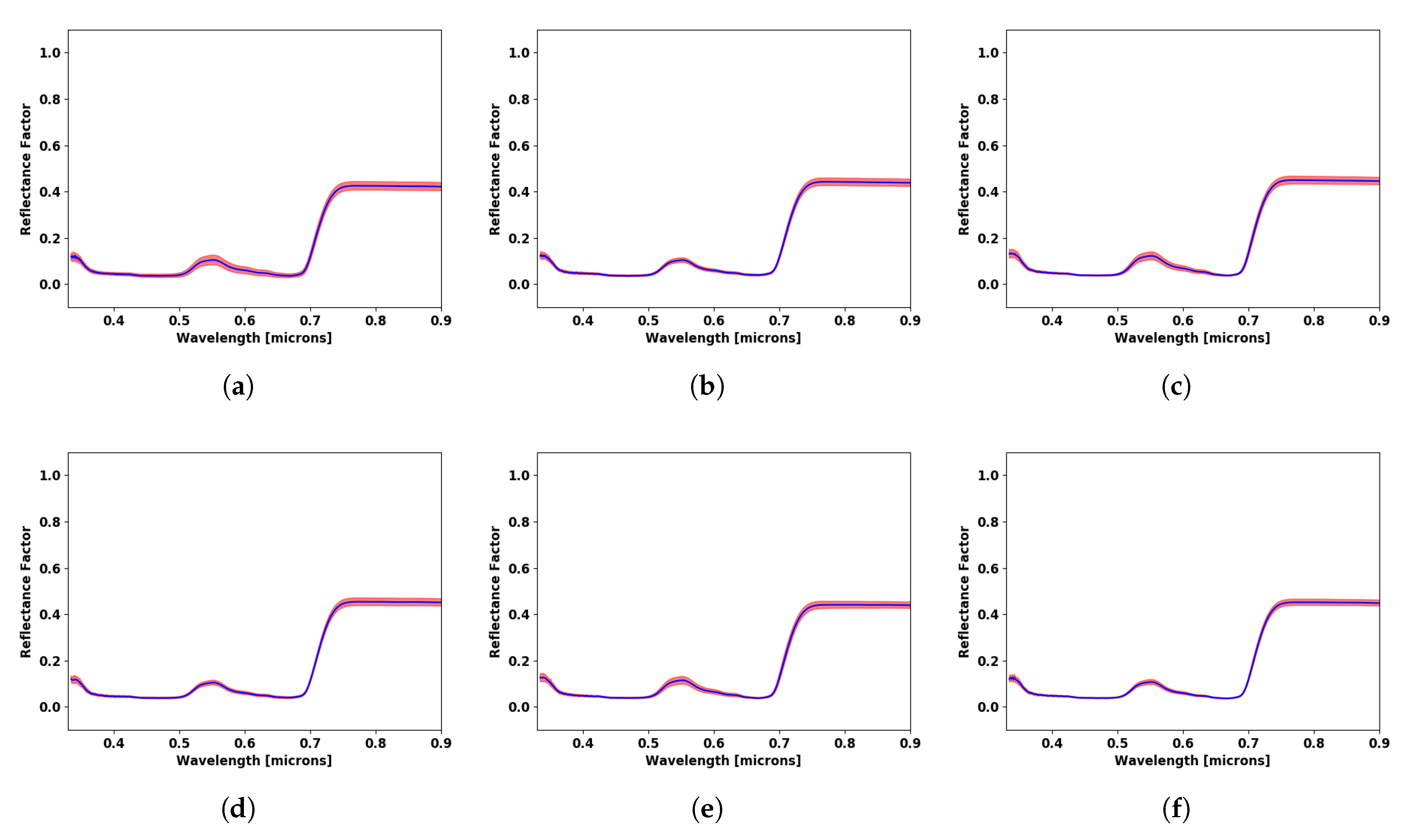
Figure 14.
Band effective reflectance factors measured from (a) Plant 1 (b) Plant 2 and (c) Plant 3 during cloudy forecast (22 September). (Left) 2 cm GSD, (Middle) 4 cm GSD, and (Right) 8 cm GSD. Reflectance values at 12:00 p.m. were not collected for Plant 2 because the cloud cover had passed. Therefore the measurements would not have been comparable with the rest of the data set that was collected on that day.

Figure 15.
Band effective reflectance factors measured from (a) Plant 4 (b) Plant 5 and (c) Plant 6 during sunny forecast (24 September). (Left) 2 cm GSD, (Middle) 4 cm GSD, and (Right) 8 cm GSD.
Figure 15.
Band effective reflectance factors measured from (a) Plant 4 (b) Plant 5 and (c) Plant 6 during sunny forecast (24 September). (Left) 2 cm GSD, (Middle) 4 cm GSD, and (Right) 8 cm GSD.

Figure 16.
Cloudy ASD NDVI results. Data was not collected for Plant 2 at 12 p.m. because the cloud cover had disappeared. Stable NDVI results seen across all three plants, all three GSDs and all five times. Average NDVI shown as scatter points, and one standard deviation displayed as error bars.
Figure 16.
Cloudy ASD NDVI results. Data was not collected for Plant 2 at 12 p.m. because the cloud cover had disappeared. Stable NDVI results seen across all three plants, all three GSDs and all five times. Average NDVI shown as scatter points, and one standard deviation displayed as error bars.

Figure 17.
Sunny ASD NDVI results. NDVI values changed across all variables: plant, GSD, time. No particular pattern is displayed. Average NDVI shown as scatter points, and one standard deviation displayed as error bars.
Figure 17.
Sunny ASD NDVI results. NDVI values changed across all variables: plant, GSD, time. No particular pattern is displayed. Average NDVI shown as scatter points, and one standard deviation displayed as error bars.

Figure 18.
Average and standard deviation reflectance captured from a leafclip for (a) Plant 1, (b) Plant 2, (c) Plant 3, (d) Plant 4, (e) Plant 5, (f) Plant 6. Plants 1, 2, and 3 were measured with the field spectroradiometer and MicaSense RedEdge-3 on the cloudy day, while plants 4, 5, and 6 were measured on the sunny day. Each plant had 30 reflectance measurements made from various leaves.

Figure 19.
NDVI computed using leafclip spectra for all six plants.

Figure 20.
Average reflectance factors computed from DIRSIG simulations (error bars represent one standard deviation). Same downward trend in reflectance is seen in the simulations.
Figure 20.
Average reflectance factors computed from DIRSIG simulations (error bars represent one standard deviation). Same downward trend in reflectance is seen in the simulations.

Figure 21.
MicaSense RedEdge-3 reflectance results on cloudy day using (a) 2-Point ELM, (b) 1-Point ELM, (c) AARR, and reflectance results on sunny day using (d) 2-Point ELM, (e) 1-Point ELM, and (f) AARR. Averages and standard deviation values computed from all captured images at their particular hours. Downward trend in reflectance can be seen across all bands as the sun rose in the sky.

Figure 22.
MicaSense average NDVI results. Significantly higher standard deviations seen in the sunny day, because of the higher variabilities measured by the RedEdge-3 sensor.
Figure 22.
MicaSense average NDVI results. Significantly higher standard deviations seen in the sunny day, because of the higher variabilities measured by the RedEdge-3 sensor.


Table 1.
MicaSense RedEdge-3 spectral bands with respective center wavelengths and bandwidth values.
Table 1.
MicaSense RedEdge-3 spectral bands with respective center wavelengths and bandwidth values.
| Band Name | Wavelengths [nm] | FWHM [nm] |
|---|---|---|
| Blue | 475 | 20 |
| Green | 560 | 20 |
| Red | 668 | 10 |
| Red Edge | 717 | 10 |
| Near IR | 840 | 40 |
Table 2.
R-squared values computed across time of day. Correlations are lower on sunny day as opposed to the cloudy day.
Table 2.
R-squared values computed across time of day. Correlations are lower on sunny day as opposed to the cloudy day.
| Cloudy Day | Sunny Day | ||||||
|---|---|---|---|---|---|---|---|
| Plant 1 | Plant 2 | Plant 3 | Plant 4 | Plant 5 | Plant 6 | ||
| GSD | 2 cm | 0.227 | 0.331 | 0.552 | 0.009 | 0.707 | 0.063 |
| 4 cm | 0.216 | 0.159 | 0.927 | 0.529 | 0.958 | 0.176 | |
| 8 cm | 0.705 | 0.849 | 0.898 | 0.155 | 0.089 | 0.022 | |
Table 3.
R-squared values computed across time of day for both days, all three reflectance conversion techniques and all five sensor bands.
Table 3.
R-squared values computed across time of day for both days, all three reflectance conversion techniques and all five sensor bands.
| Cloudy Day | Sunny Day | |||||
|---|---|---|---|---|---|---|
| 2-Point ELM | 1-Point ELM | AARR | 2-Point ELM | 1-Point ELM | AARR | |
| Blue | 0.020 | 0.820 | 0.652 | 0.853 | 0.939 | 0.807 |
| Green | 0.654 | 0.808 | 0.713 | 0.950 | 0.388 | 0.578 |
| Red | 0.125 | 0.848 | 0.710 | 0.918 | 0.871 | 0.725 |
| RE | 0.930 | 0.939 | 0.751 | 0.985 | 0.946 | 0.911 |
| NIR | 0.935 | 0.949 | 0.903 | 0.686 | 0.810 | 0.813 |
Table 4.
MicaSense RedEdge-3 and DIRSIG average (standard deviation) reflectance factors measured at 08:00 a.m. and 12:00 p.m. DIRSIG simulations do not match with RedEdge-3 results because DIRSIG does not compute the Fresnel reflection.
Table 4.
MicaSense RedEdge-3 and DIRSIG average (standard deviation) reflectance factors measured at 08:00 a.m. and 12:00 p.m. DIRSIG simulations do not match with RedEdge-3 results because DIRSIG does not compute the Fresnel reflection.
| 08:00 a.m.-Sunny | 12:00 p.m.-Sunny | |||||||
|---|---|---|---|---|---|---|---|---|
| 2-Point ELM | 1-Point ELM | AARR | DIRSIG | 2-Point ELM | 1-Point ELM | AARR | DIRSIG | |
| Blue | 0.025 (0.039) | 0.032 (0.039) | 0.027 (0.033) | 0.039 (0.046) | −0.021 (0.026) | 0.035 (0.022) | 0.030 (0.019) | 0.037 (0.027) |
| Green | 0.094 (0.110) | 0.096 (0.109) | 0.119 (0.134) | 0.054 (0.066) | 0.031 (0.055) | 0.085 (0.047) | 0.096 (0.053) | 0.046 (0.038) |
| Red | 0.033 (0.057) | 0.034 (0.057) | 0.042 (0.070) | 0.078 (0.087) | −0.011 (0.035) | 0.046 (0.030) | 0.050 (0.033) | 0.070 (0.051) |
| RE | 0.255 (0.260) | 0.257 (0.254) | 0.342 (0.339) | 0.169 (0.182) | 0.165 (0.118) | 0.200 (0.097) | 0.251 (0.122) | 0.144 (0.110) |
| NIR | 0.534 (0.323) | 0.519 (0.302) | 0.694 (0.404) | 0.199 (0.209) | 0.459 (0.216) | 0.430 (0.168) | 0.507 (0.198) | 0.173 (0.129) |
© 2019 by the authors. Licensee MDPI, Basel, Switzerland. This article is an open access article distributed under the terms and conditions of the Creative Commons Attribution (CC BY) license (http://creativecommons.org/licenses/by/4.0/).
Share and Cite
MDPI and ACS Style
Mamaghani, B.; Saunders, M.G.; Salvaggio, C. Inherent Reflectance Variability of Vegetation. Agriculture 2019, 9, 246. https://0-doi-org.brum.beds.ac.uk/10.3390/agriculture9110246
AMA Style
Mamaghani B, Saunders MG, Salvaggio C. Inherent Reflectance Variability of Vegetation. Agriculture. 2019; 9(11):246. https://0-doi-org.brum.beds.ac.uk/10.3390/agriculture9110246
Chicago/Turabian StyleMamaghani, Baabak, M. Grady Saunders, and Carl Salvaggio. 2019. "Inherent Reflectance Variability of Vegetation" Agriculture 9, no. 11: 246. https://0-doi-org.brum.beds.ac.uk/10.3390/agriculture9110246
Note that from the first issue of 2016, this journal uses article numbers instead of page numbers. See further details here.