Intercropping Simulation Using the SWAP Model: Development of a 2×1D Algorithm


1
Soil Physics Laboratory, Center for Nuclear Energy in Agriculture, University of São Paulo, PO Box 96, Piracicaba SP 13416-970, Brazil
2
Department of Environmental Sciences, Wageningen University and Research Centre, PO Box 47, 6700 AA Wageningen, The Netherlands
*
Author to whom correspondence should be addressed.
Agriculture 2019, 9(6), 126; https://0-doi-org.brum.beds.ac.uk/10.3390/agriculture9060126
Submission received: 21 May 2019
/
Revised: 8 June 2019
/
Accepted: 12 June 2019
/
Published: 16 June 2019
Abstract
:Intercropping is a common cultivation system in sustainable agriculture, allowing crop diversity and better soil surface exploitation. Simulation of intercropped plants with integrated soil–plant–atmosphere models is a challenging procedure due to the requirement of a second spatial dimension for calculating the soil water lateral flux. Evaluations of more straightforward approaches for intercrop modeling are, therefore, mandatory. An adaptation of the 1D model Soil, Water, Atmosphere and Plant coupled to the World Food Studies (SWAP/WOFOST) to simulate intercropping (SWAP 2×1D) based on solar radiation and water partitioning between plant strips was developed and the outcomes are presented. An application of SWAP 2×1D to maize–soybean (MS) strip intercropping was evaluated against the monocropping maize (M) and soybean (S) simulated with the 1D model SWAP/WOFOST, and a sensitivity analysis of SWAP 2×1D was carried out for the intercropping MS. SWAP 2×1D was able to simulate the radiation interception by both crops in the intercropping MS and also to determine the effect of the radiation attenuation by maize on soybean plants. Intercropped plants presented higher transpiration and resulted in lower soil evaporation when compared to their equivalent monocropping cultivation. A numerical issue involving model instability caused by the simulated lateral water flux in the soil from one strip to the other was solved. The most sensitive plant parameters were those related to the taller plant strips in the intercropping, and soil retention curve parameters were overall all significantly sensitive for the water balance simulation. This implementation of the SWAP model presents an opportunity to simulate strip intercropping with a limited number of parameters, including the partitioning of radiation by a well-validated radiation sharing model and of soil water by simulating the lateral soil water fluxes between strips in the 2×1D environment.
1. Introduction
Intercropping is a method employed for agricultural sustainability in which two or more plant species are simultaneously cultivated together on the same land [1,2,3] Intercropping systems are favored by a better land occupation, a decrease in the use of agrochemicals, better soil conservation, and yield diversification, among other benefits [4,5,6,7]. Management challenges for intercropping include the use of an optimum plant density, cultivation design or plant strip widths, and the best times of seeding for each of the crops to maximize crop productivities [8]. A better strategy of intercropping cultivation can be facilitated and accomplished with multi-species cropping system modeling [9].
Models for intercropping systems have been developed using several approaches [10] simulating the competition of intercrop plants mainly for water and radiation. The competition for radiation by intercropped plants is, however, the main process taken into account in modeling studies [11,12,13,14,15,16,17]. Chimonyo [18] pointed out the difficulties of evaluating the root systems and water extraction dynamics of multicropping systems are the main reason for the modeling of the processes belowground to be put aside. Another reason for avoiding the belowground modeling in intercropping is the difficulty of integrating two spatial dimensions for the simulation of the vertical and horizontal soil water fluxes [19].
Approaches in which the belowground resource sharing can be simulated simply and feasibly are highly desirable [20,21]. Chen [22] evaluated the concept that the lateral movement of water within strips of an intercropping occurs predominantly when a gradient of soil water content exists between strips. This procedure, physically based on Darcy’s law, was used also in Karray [23] for modeling the water exchange between plots of olive-trees and annual crops. Such a simple concept can facilitate the modeling of the lateral soil water flow in the strip intercropping with 1D-models in which only the vertical coordinate is simulated.
The hydrological model Soil, Water, Atmosphere and Plant (SWAP) [24] coupled to the crop growth model World Food Studies (WOFOST) [25] simulates the hydrological processes and plant growth in cropping systems and provides detailed water balances and crop productivity predictions. SWAP/WOFOST is a 1D model, simulating flow processes in the vertical direction. Results may be considered representative of a plot or a field-scale region if soil, cropping system, and meteorological data are considered spatially uniform. Implicitly, SWAP/WOFOST is unable to simulate two crops growing together and partitioning water and radiation, like in intercropping or agroforestry. Intercropping simulation with SWAP could be accomplished, however, by simulating two soil-plant modules simultaneously, having a third routine controlling the interchange of water and radiation between plants.
In this context, we aimed to develop a modified version of SWAP/WOFOST that allows simulating upper and belowground resources partitioning between intercropped plants. In the present evaluation, we considered that in each intercropping strip the plant and root system are limited to the respective soil profile as well as to the aerial portion of the strip. Hence, plants can be simulated separately in modules, sharing radiation in accordance to plant strip geometry, and interchanging water between modules by a lateral flow dependent on the soil hydraulic status of the soil layers in both strips. The new version of SWAP/WOFOST combines the robustness of the existing 1D model to the possibility of simulating the water balance components and crop growth in an intercropping scenario. Model theory and assumptions are described and tested for a hypothetical case of relay-strip intercropping.
2. Material and Methods
2.1. Model Description
2.1.1. SWAP 2×1D
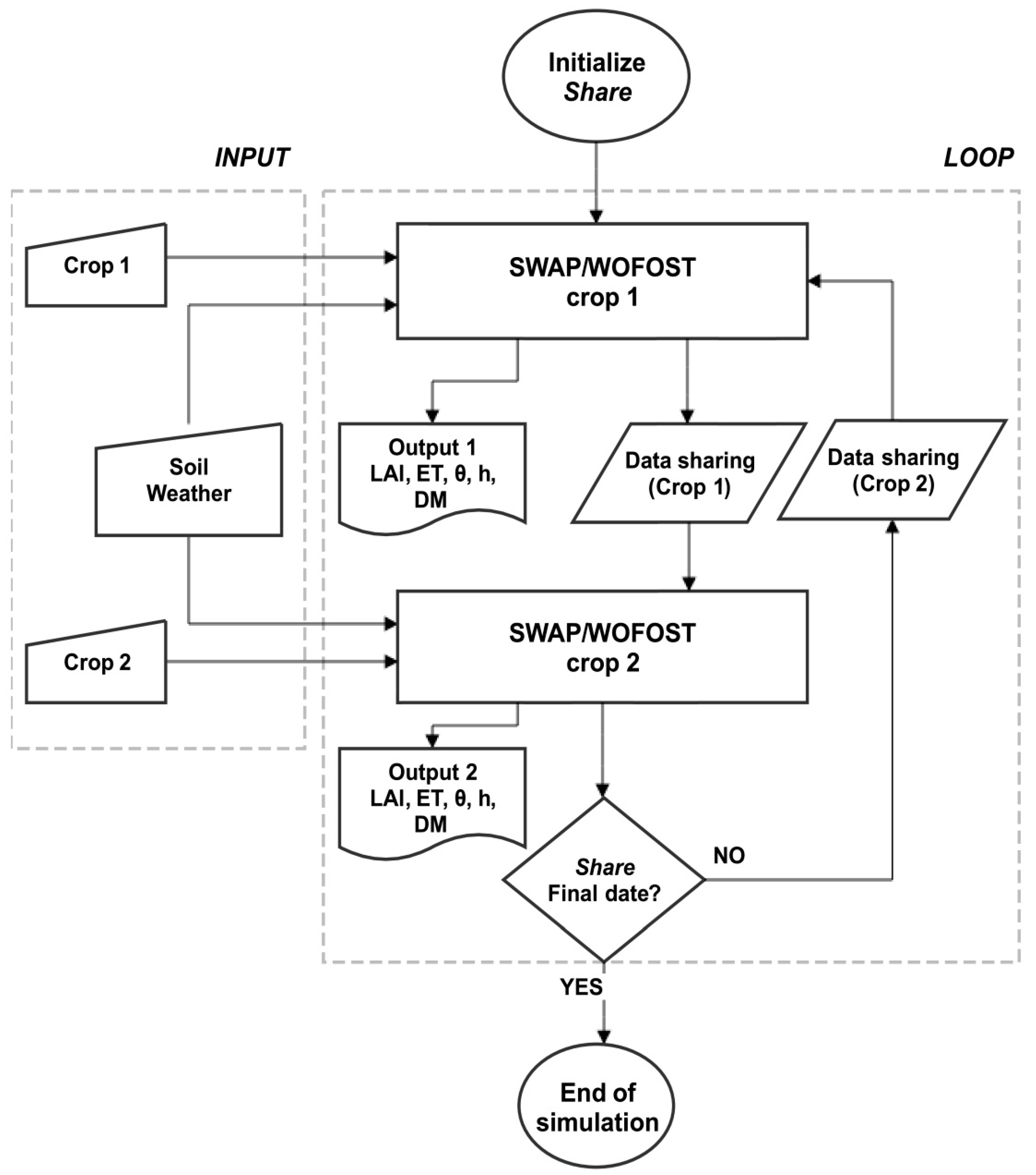
The intercropping simulation model SWAP 2×1D consists of two joined conventional SWAP/WOFOST (1D) (version 4.0.4) modules, capable of interchanging data of plant and soil-water fluxes after every 24 h simulation period. The daily loops of simulation (the LOOP process in Figure 1) for the desired period of intercropping cultivation with SWAP 2×1D are executed by an external routine named Share in combination with a batch file. Reading and storage of data (INPUT process) takes place once at the onset of a simulation. Output data are written to default SWAP document files every loop until the end of the simulation.
2.1.2. Radiation Interception
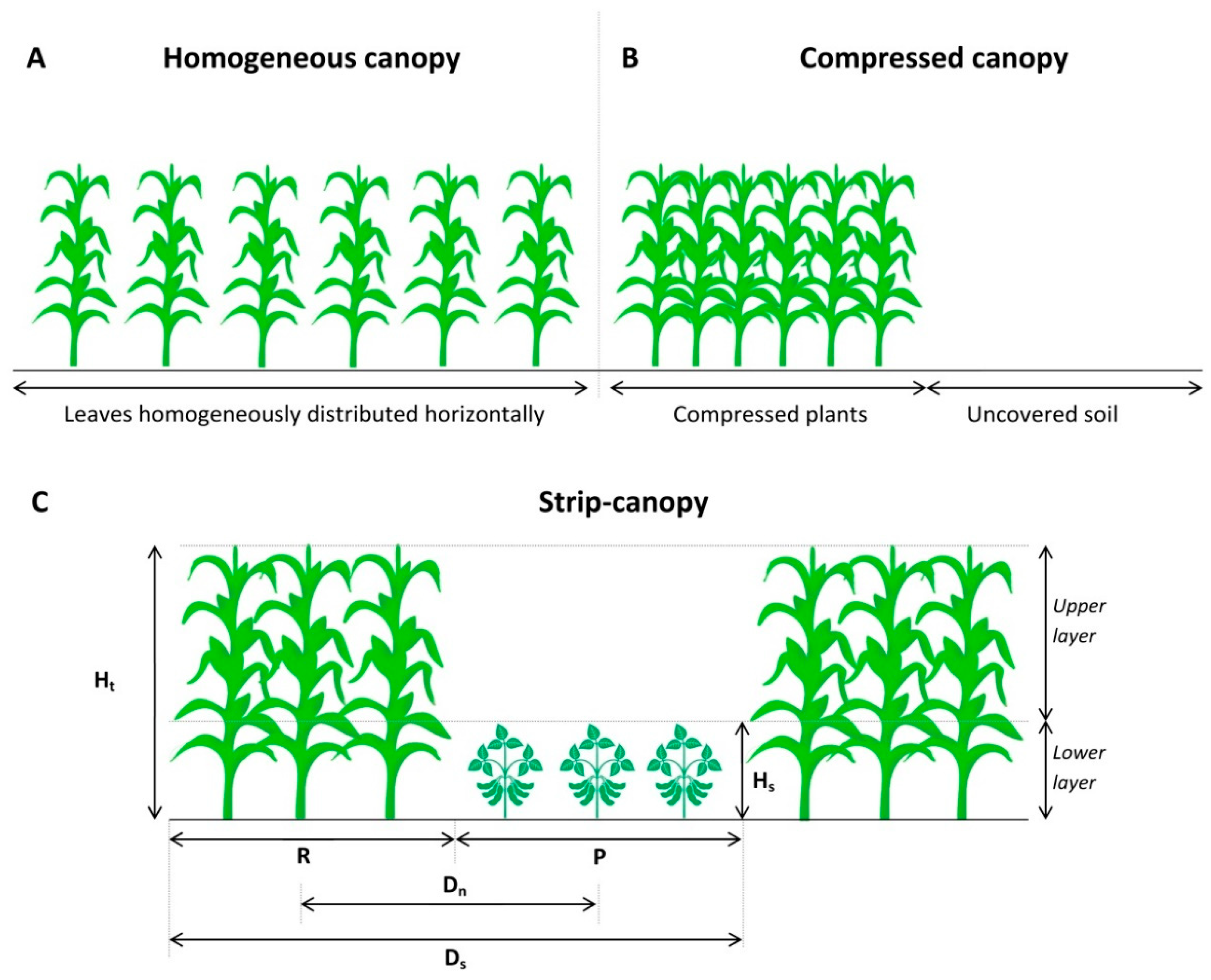
A radiation interception model for relay-strip intercropping based on a canopy formed by block-structures was developed by Pronk [15], and evaluated by Gou [11,12]. The radiation interception by strip intercropping plants as described by Pronk [15] and Gou [11,12] remains in between the radiation intercepted by a homogeneous and a compressed canopy. In a homogeneous canopy (Figure 2), leaf areas are considered homogeneously distributed horizontally, like in mixed pastures. The radiation interception of a homogeneous canopy is higher than the radiation interception by a strip intercropping canopy for two main reasons: (1) A homogenous canopy model does not take into account the soil paths present in the relay-strip intercropping when only one crop species is in the field; and (2) the border effects of the strips are not taken into account in the homogenous canopy model. In a compressed canopy scenario, the plant rows and the soil paths can be thought of as two separate units: (1) plant rows without paths and (2) uncovered soil paths, both occupying a complementary fraction of the total soil area (Figure 2). In the compressed type canopy model, the radiation is partly intercepted by the canopy with plants very close to each other, and partly by the uncovered soil. The strip-canopy radiation interception is larger than in a compressed canopy because the strip-border plants are more exposed to the radiation and are more numerous than in the compressed canopy [11,12].
In a relay-strip intercropping, one of the canopies is taller than the other and referring to radiation interception the taller one is subdivided in an upper part (above the shorter canopy) and a lower part, according to the computation algorithm described in the following.
The fraction of the intercepted radiation by a strip-canopy (ft) is in between a maximum value, the radiation interception fraction by a homogeneous canopy, and a minimum value equal to the addition interception fraction by a compressed canopy. ft is calculated as the weighted average of the radiation interception fraction by a homogeneous and a compressed canopy (Figure 2A,B), as described by Gou [11]:
Fractions fh and fc are calculated by:
The leaf area index (LAI) of a compressed canopy LAIc is defined by:
The weighting factor w in Equation (1), which represents the relative contribution of the homogeneous and compressed parts, is defined by:
In this equation, SP is the fraction of radiation reaching the path between strips soil surface, and SR the fraction of radiation reaching the soil under the strips:
IP is the fraction which represents the spatial integration of radiation reaching the path between strips, and IR the fraction of representing the spatial integration of the radiation reaching the strip [15]. IP and IR are dependent on the crop plantation form (P and R, respectively) and plant height (H). IP and IR are view factors of the path and plant strip, respectively, and can be calculated according to [26]:
To calculate IP and IR in an intercropping system, the plant height of the taller plant species Ht is used to substitute H in Equations (8) and (9).
To calculate the radiation interception fraction of intercropping plants with different heights, the intercropping canopy is divided into two layers limited by the shorter (Hs) and the taller (Ht) plant height (Figure 2C). The upper layer is limited at the top by Ht and at the bottom by Hs. The lower layer is limited at the top by Hs, and at the bottom by the soil surface. The lower layer is composed by both crop strips alternated. The LAI of the taller canopy is separated into an upper part (Equation (10)), referring to the upper layer of the canopy, and a lower part (Equation (11)) belonging to the lower layer of the canopy.
In these equations, LAIt,u is the portion of the LAI of the taller plant in the upper layer, and LAIt,l is the portion of the LAI in the lower layer. The compressed form of Equations (10) and (11) can be obtained similarly, replacing the homogeneous plant LAI by the respective LAI for the compressed canopy (LAIc).
The fraction of the radiation intercepted by the taller crop in the intercropping (Figure 3B) is the sum of radiation intercepted by the taller plant in the upper layer (ft,u) and in the lower layer (ft,l) of the canopy:
The fraction of the radiation intercepted by the taller plant in the upper layer ft,u is calculated using Equations (1)–(9). The fraction of the radiation intercepted by the taller plant in the lower layer of the canopy is calculated considering plants to have a compressed arrangement in the field. The lower layer of the canopy consists of the lower part of the taller crops sharing space with the shorter plants. The lower part of the taller plants receives the fraction of the radiation transmitted through the upper part of the taller plant strip (SRt,u):
The fraction of the radiation intercepted by the shorter plants is calculated according to:
where SPt,u is the fraction the directly incident radiation transmitted through the taller plant strips to the soil path:
In the case of intercropping species with equal heights (Figure 3C), the fraction of the radiation intercepted by each plant strip is calculated according to:
For all plant height combinations in the simulations, the fraction of radiation intercepted by the soil (fg) is calculated as:
2.1.3. Atmospheric Vapor Fluxes
Potential plant transpiration Tp (cm) and soil evaporation Ep (cm) are predicted in the SWAP model using the Penman–Monteith equation [27]. Plant species growing together affect each other’s Tp and Ep. The fraction ft,i is plant-dependent; therefore, plant transpiration is calculated for each crop (Tp,i) in the simulation unit according to the Penman–Monteith equation with the effect of the presence of the other plant species in the field accounted for by ft,i in Tp, and the fraction of the radiation intercepted by the soil (fg) controls the radiation and the aerodynamic terms [28]:
The aerodynamic terms of the Penman–Monteith equation (ra,c,i and ra,s) are calculated according to:
In the SWAP model, the actual transpiration Ta,i (cm) is calculated as a function of the soil root distribution and Tp,i, and the combined effect of water, oxygen and salt stress are accounted [24]. In SWAP 2×1D, the assumption of the roots overlapping in the intercropping [29] is not considered and the root distribution model is the SWAP default. The water interception Pin,i (cm) by the canopy of each plant in the intercropping unit is obtained by the method of Von Hoyningen-Hüne and Braden [24]. To distribute Pin,i between plant species canopy, the ft,i factor of each crop type is added to the Pin,i calculation according to:
2.1.4. Lateral Soil Water Flux
To calculate the lateral exchange of water between both intercropping strips (ql,d, cm d−1) in SWAP 2×1D, the Darcian flow based on the pressure head gradient between two equal-level compartments and their average soil hydraulic conductivity on a daily basis is considered:
The lateral water balance component is calculated at the end of each simulated 24 h period and then added to the water balance of both SWAP 2×1D modules. SWAP uses a variable but smaller time step (between 1.0∙10−6 and 0.8 d) to calculate the soil water fluxes and solve the Richards equation, and the addition of a daily water flux at a relatively large time step may cause numerical instability or lead to non-convergence of the numerical scheme in the subsequent time step. To avoid this, a limiting lateral water flux qlim,d is defined as:
The actual lateral flux per compartment (qd) applied in SWAP 2×1D is calculated based on qlim,d and ql,d according to:
The lateral flux qd is adjusted to the plant-specific below ground coverage Bc,i (Equation (27)). Bc,i is the proportion of land coverage by the plant species intercropped and its value represents relatively the plant root dominance in the soil profile. The coverage coefficient Bc,i is an input value specified by the user, and the Bc,i values of both plants intercropped must sum up to 1. The relative plant root dominance in soil influences the exchange of water between SWAP 2×1D modules:
The total horizontal soil water flux QL,i (cm d−1) is calculated as the daily sum of compartment lateral fluxes qd,i:
2.1.5. Water Balance
The water balance is initially independently calculated for both strips as:
where indices 1 and 2 refer to strips with crops 1 and 2.
The water balance is subsequently calculated for the intercropping simulation unit in SWAP 2×1D from both modules 1 and 2. The intercropping water balance is equal to ∆Sint (Equation (31)), and the sum of ∆S1 and ∆S2 multiplied by the respective values of Bc for strip 1 (Bc,1) and strip 2 (Bc,2):
2.2. Model Evaluation
To evaluate the performance of SWAP 2×1D, a scenario with maize (Zea mays L.) and soybean (Glycine max L.) was simulated using both the single crop SWAP 1D and the strip intercropping SWAP 2×1D. Some details about the simulated scenarios are presented in Table 2 and Figure 4.
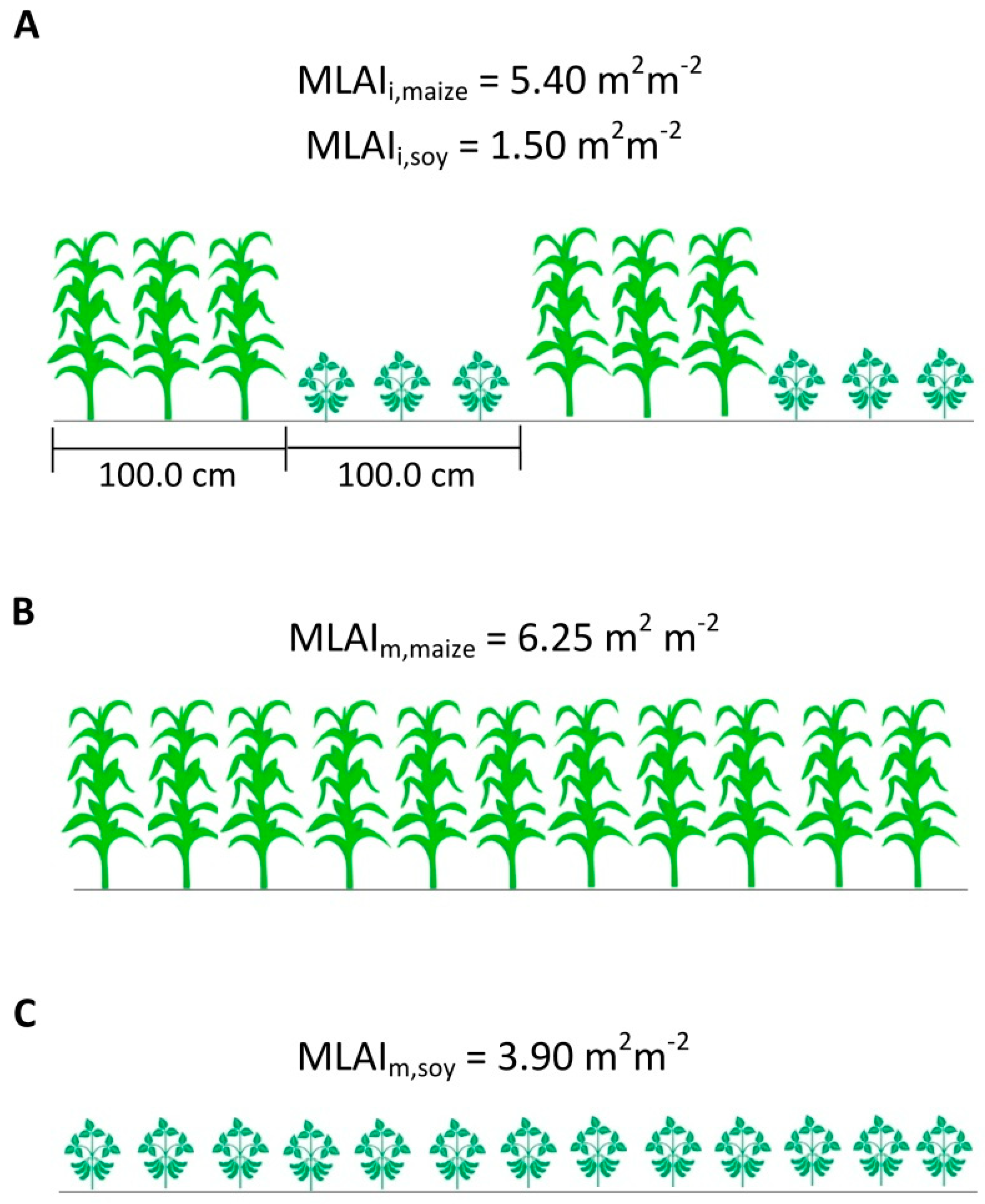
For scenarios MS and M, the maize crop cycle started on January 1 (day 1) and ended on April 22, 2015 (day 112), and for MS and S, soybean was simulated to grow from February 20 (day 51) to July 12, 2015 (day 193). To include the entire maize and soybean cycles in the simulations, the simulated period for all scenarios was from January 1 to July 12 (193 days). The distance between two strips of maize (Ds,maize) was 2.0 m in the intercropping scenarios maize-soybean (MS). Ds, strip (R) and path (P) widths are input values for the radiation distribution module in SWAP 2×1D. The strip width R and soil strip width P were both equal to the average 1.0 m and were kept constant during the cropping seasons. R and P were obtained by multiplying plant coverage (Bc) by the distance between rows (Ds). The number of plant rows is absent in the simulations of SWAP 2×1D or SWAP 1D, but it is accounted for by the LAI. Default plant development parameters were used in the WOFOST crop file (Table 3). Plant H, Rd, and specific leaf area LA were set based on experimental data reported in the scientific literature [29,30,31]. For maximum rooting depths Rd,m, 100 cm was used both for maize and soybean. The soil was of sandy-clay texture as described in de Jong van Lier [32], with hydraulic properties in Table 4. The soil profile depth is 112 cm, and the profile is subdivided into four sub-layers: 0–12 cm, 12–32 cm, 32–62 cm, and 62–112 cm. Free drainage of the soil profile was used as the bottom boundary condition.
Weather data were taken from the weather station of the University of São Paulo in Piracicaba, Brazil (22°42′ S, 47°38′ W). The total precipitation during the cropping season was 289 mm. No irrigation was applied in the simulation scenarios.
2.3. Sensitivity Analysis
To evaluate the sensitivity of output variables (Vf) to soil and plant parameters, a sensitivity analysis was performed for the intercropping of maize and soybean (Table 1). The evaluated output variables are: radiation interception fraction by the intercrop (ft), actual crop transpiration (Ta), actual soil evaporation (Ea), lateral soil water flux (QL) and flux below the root zone (Qb). Each of these output variables were evaluated using the relative partial sensitivity index η:
in which Vf is the evaluated output variable, Vs is the new value of the output variable after a selected parameter was changed, and (Vf − Vs) the difference of an output variable due to the change of parameter p. The reference Vr is the average of Ta, Ea, QL, and Qb output values for water fluxes, and the average of the output values of ft for the radiation interception simulated with the default (reference) parameters values. To calculate η, the selected parameter was changed by 1% (Δp/p = 0.01) while the others were maintained at their default value. The reference value Vr was 9.5 cm for the soil fluxes variables Ta, Ea, QL, and Qb, and 0.38 for the radiation interception ft. A variable with |η| ≥ 0.5 was considered to have high sensitivity to the parameter evaluated.
3. Results and Discussion
3.1. LAI and Radiation Interception
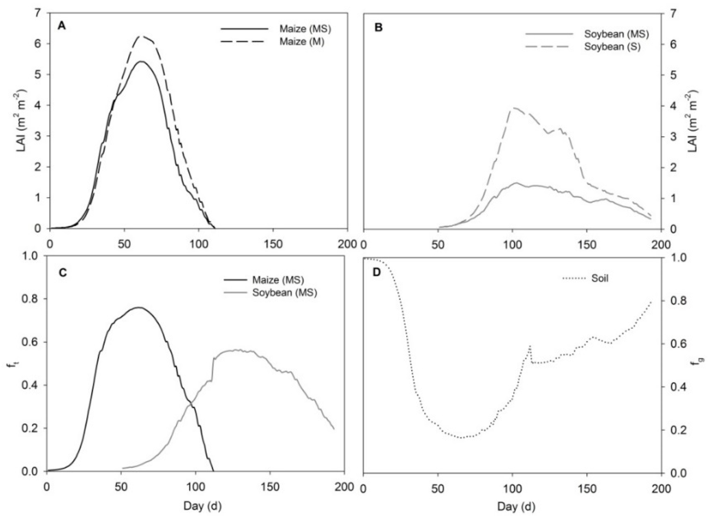
Intercropped maize LAI simulated by SWAP 2×1D was lower than in maize monocropping (Figure 5A) for most of the simulation period. This difference in LAI can be explained since in the intercropping maize–soybean plants of soybean were occupying half of the cultivation area covered by maize plants in the monocropping. Maize LAI was calculated for the whole cultivated area in SWAP 2×1D and for that reason it is lower than the monocropping maize LAI predicted by SWAP 1D. Intercropped soybean plants were simulated to grow together with taller plants of maize and to receive less radiation compared to the monocropping cultivation of soybean, another reason for soybean intercropping LAI to be reduced (Figure 5B). SWAP 2×1D was able to reproduce the reduction in the intercrop LAI compared to the monocropping system, similarly to the behavior of the intercropping LAI observed by Gou [11] and Liu [34].
The fraction of radiation interception (ft) in maize as a function of time showed similar to the intercropping LAI, showing the low interference of the shorter soybean plants in this scenario. Soybean ft increased suddenly on day 112 because maize plants were harvested on this date and no longer covered the remaining soybean plants. The maximum ft by the intercropped maize canopy simulated by SWAP 2×1D was 0.80 at LAI 5.40 m2 m−2 and maximum ft by soybean canopy was 0.49 at LAI 1.38 m2 m−2 (Figure 5C).
The fraction of radiation intercepted by the soil surface (fg) suddenly decreased at the end of maize cycle on day 112 (Figure 5D). After maize harvest, more radiation reached the soil, attenuated only by the soybean plants. SWAP 2×1D does not consider the possibility of existing plant shoots and remaining biomass over the soil after harvest, which could result in a smaller value of fg.
3.2. Transpiration and Evaporation Fluxes
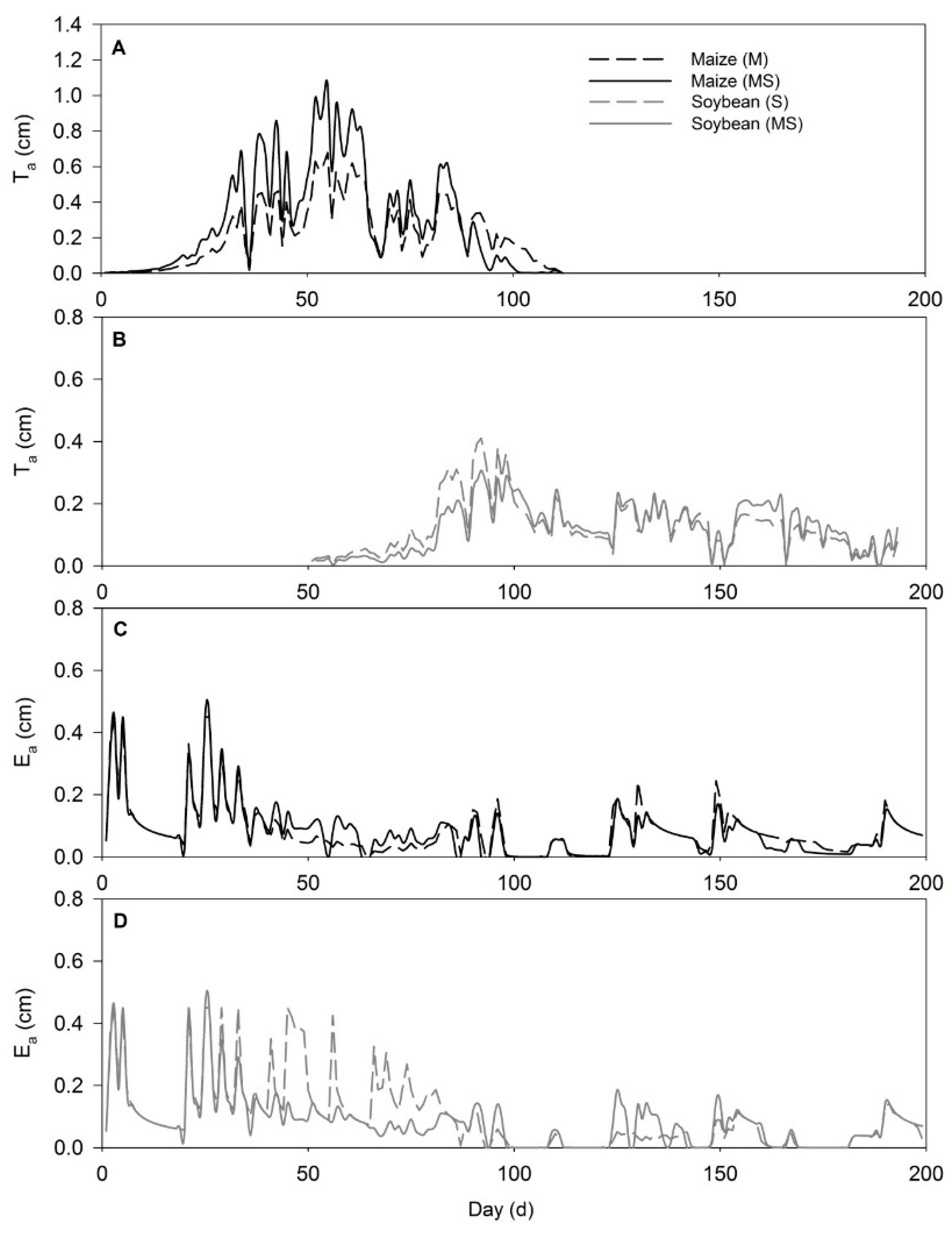
Intercropped maize Ta is higher than maize monocropping Ta for most of the cultivation period (Figure 6A). The maximum Ta for intercropped maize is 1.05 cm d−1 and for maize monocropping is 0.68 cm d−1 at the end of the vegetative cycle (day 55). The effect of shadowing of soybean by maize is observed between days 50 and 100, when soybean (MS) Ta is 0.05 cm d−1 and monocropping soybean (S) Ta is 0.14 cm d−1. The maximum Ta for intercropped soybean is 0.30 cm d−1 and for monocropping soybean is 0.41 cm d−1 (on day 92, Figure 5B). The sudden reduction in soybean monocropping and intercropping Ta after day 95 is a response to water shortage, however. On average, intercropped soybean Ta is reduced by 0.05 cm d−1 and monocropping soybean Ta by 0.06 cm d−1 due to water shortage from day 95 to 192.
The transpiration fluxes obtained in these hypothetical scenarios were not validated, but the intercropped plant transpiration behavior (Ta) simulated by SWAP 2×1D in comparison to their monocropping Ta values was in agreement with the behavior of the intercropping wheat-maize and wheat-sunflower compared to their monocropping systems as obtained by Miao [31].
Intercropped maize (MS) soil Ea predicted by SWAP 2×1D was correspondent to maize monocropping (M) soil Ea in most of the season except a few periods (Figure 6C). From day 50 to 80, differences in MS and M Ea are probably an effect of distinct plant transpiration in both scenarios. Between days 150 to 200, the soil was uncovered in scenario M, while in MS the soil evaporation was affected by soybean strips and their partial interception of the incoming radiation, causing the difference in evaporation between M and MS. The intercrop effect of maize plants on soybean Ea are simulated by SWAP 2×1D (Figure 6B,D). From day 41 to 80, in the intercropping period, average Ea of the soil under intercrop soybean is 0.04 cm d−1 while Ea in monocropping soybean is 0.20 cm d−1 (Figure 6D).
3.3. Lateral Soil Water Flux
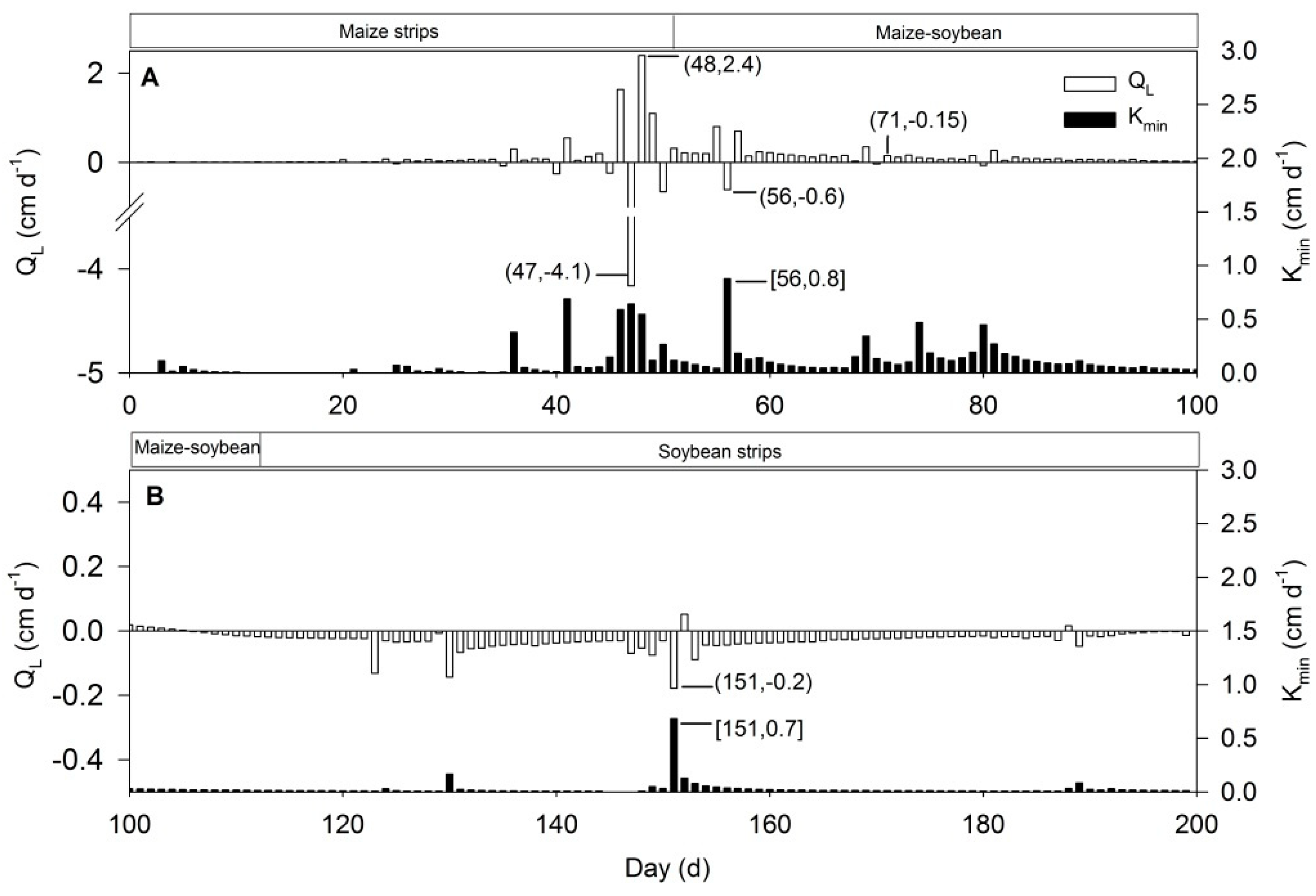
The higher water demand by maize plants made SWAP 2×1D predict a lateral water flow (average 0.15 cm d−1) from the soybean towards the maize strips (Figure 7A) during most of the time until day 112. In the first 20 days of maize development, water was supplied by the frequent rainfall events and no significant lateral flow developed. Intercropped maize water demand increased, making the lateral water flow to increase from day 20 to 48. As QL is governed by soil pressure head gradients as well as by Kmin, peak events of QL (e.g., on days 47, 48, 56 and 151) were caused by events of high precipitation causing an instantaneous increase of Kmin (Figure 7A,B). After the end of the maize cycle (day 112), water flows laterally at an average 0.03 cm d−1 towards the soybean soil region until the end of the soybean crop season.
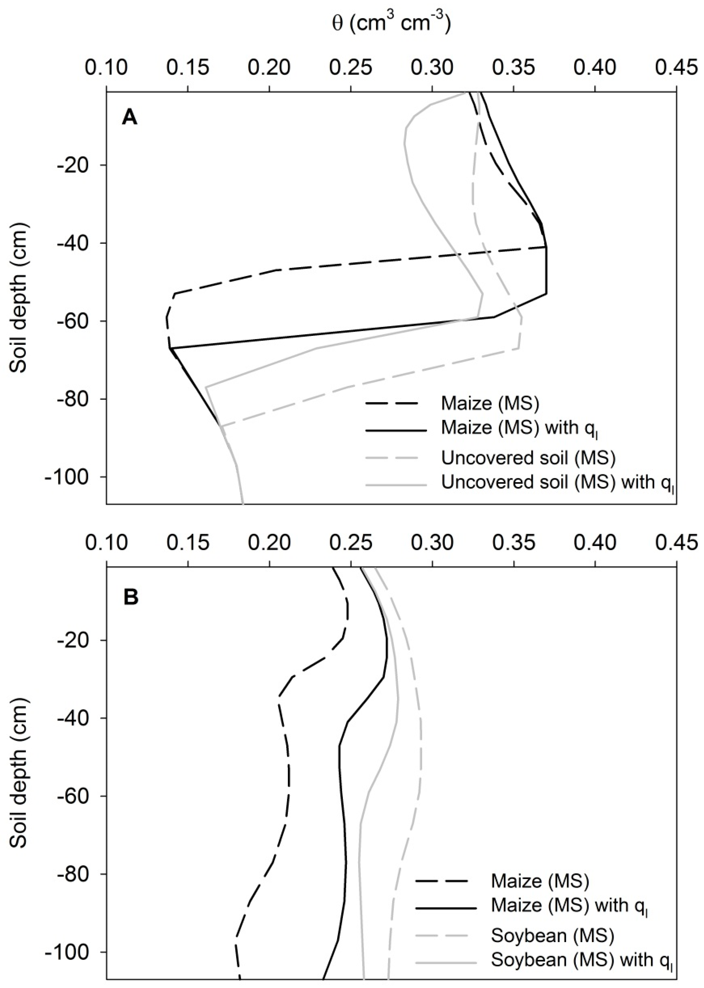
The significance of the lateral water flow for soil water availability in the intercropping (MS) is observed comparing the soil water content profiles of maize and soybean predicted by SWAP 2×1D with and without the horizontal soil water exchange (Figure 8). Within the first 48 days, maize strips are cultivated in between paths of uncovered soil (Figure 8A), and the soil water content (θ) in the 55–65 cm depth region in maize soil profile is greater than in maize (MS) simulation with no lateral flux. The θ of the soil path (strip of uncovered soil) in the soil depth 0–80 cm for the simulations with lateral water flow is lower than the θ of the soil profile in the simulations without the lateral water flow. On day 71, the effect of the lateral soil water flow on θ of the intercropping soil profile is evident (Figure 8B). Soybean soil θ distribution tends to be lower in the simulation with lateral flux since water was flowing preferentially from soybean to maize until day 71.
3.4. Water Balance
The water balance components of the intercropping MS and monocropping maize (M) and soybean (S) are shown in Table 5. The canopy water interception (Pi), soil evaporation (Ea), and bottom flux (Q) for the intercropping simulated with SWAP 2×1D were similar to the average of the monocropping water balance components simulated with SWAP 1D. MS intercropping potential and actual transpiration rates (Tp and Ta) predicted by SWAP 2×1D are higher than the weighted averages Ta and Tp of the monocropping maize and soybean obtained with SWAP 1D. Consequently, other components of the water balance, the water storage (S) and Qb for the intercropping MS, are reduced in comparison to average of the monocropping maize and soybean. The actual and potential evapotranspiration (ETa and ETp) were similar for the scenarios M, S, simulated with SWAP 1D, and MS with SWAP 2×1D.
The lateral water flux (QL) simulated with SWAP 2×1D for the whole period of MS intercropping is 5.0 cm, from the soybean to the maize soil strip. QL is significantly low compared to the other components of the water balance ETa, Ta and Ea. However, the low exchange of water laterally observed is the resultant sum of the daily positive (soybean to maize) and negative (maize to soybean) lateral fluxes. Positive lateral fluxes QL in the soil under maize occurred frequently in the first half of the whole simulation period (Figure 7). With the end of maize cycle, the lateral water flux was frequently in the soybean direction. The maximum QL was 4.1 cm d−1, and the water flow from maize to soybean strips. The wet period during maize-strips and MS intercropping is also predominant for the resultant low lateral flux. A scenario of intercropping in which water is not available sufficiently and plants are sown at the same time can result in distinct lateral flow behavior and resultant QL.
3.5. Sensitivity Analysis
Intercropped maize potential transpiration (Tp) is sensitive to maize radiation use efficiency (RUE), albedo (Cref), maximum increase of LAI (RLAI), and coefficients of light extinction (kdif and kdir). Since Tp is directly related to the radiation interception by the plant, an increase in Cref results an increase in the radiation reflection and decrease in the radiation absorption and, consequently, a reduction in Tp. An increase in RUE, RLAI, kdif, and kdir increased Tp due to an improvement in the conversion of the incoming radiation.
Maize plant parameters albedo (Cref) and maximum increase of LAI (RLAI) show significant influence on maize actual transpiration (Ta), lateral flux (QL), and bottom flux (Qb). Accordingly, changes in maize Cref and RLAI affect intercropped soybean QL and Qb significantly. Intercropped maize QL and Qb are sensitive to Cref and RLAI, as a consequence of Ta behavior in the sensitivity analysis.
Maize Ta is affected by the saturated soil water content (Өs), shape parameters of the soil water retention curve a and n, and the saturated hydraulic conductivity (Ks), which are the parameters that change effectively the soil water availability for plants in SWAP. The lateral flux QL and bottom flux Qb were sensitive to most of the evaluated soil parameters.
The variables presented in Table 6 had no significant sensitivity to soybean parameters in the evaluation, and their results were, therefore, omitted. The highest sensitivities (η > 2) of maize and soybean simulations were obtained for Өs and RLAI.
Most of the plant and soil parameters included in Table 6 are important for the simulation of intercropping MS. These parameters are recommended to be adjusted in a calibration and validation processes of the model SWAP 2×1D. Nevertheless, the sensitivity of the output variables available in Table 6 refers to SWAP 2×1D simulated with the default parameters and meteorological conditions in the current hypothetical scenario. The sensitivity of the output variables to the selected parameters may be different in a distinct scenario.
4. Conclusions
Radiation and soil water sharing subroutines were implemented in the model SWAP/WOFOST 1D for the simulation of strip intercropping cultivation. We presented theory and concepts used in the newly developed model SWAP 2×1D and simulated hypothetical scenarios to discuss the significance of simulating the lateral soil water flux in the intercropping in addition to the radiation sharing between plants. SWAP 2×1D was capable of simulating above- (light) and belowground (water) interactions in strip intercropping.
The lateral water flow between soil strips in the intercropping scenario was relatively low compared to other components of the water balance on a cumulative basis. Daily values, however, were of the same order of magnitude as transpiration and evaporation rates. The effect of the lateral water exchange on the soil water storage of the intercropping was shown to be significant.
Author Contributions
Conceptualization, V.M.P., J.C.v.D. and Q.d.J.v.L.; methodology, V.M.P. and J.C.v.D.; validation, V.M.P., J.C.v.D., Q.d.J.v.L. and K.R.; software, V.M.P. and J.C.v.D.; formal analysis, V.M.P., J.C.v.D., Q.d.J.v.L., and K.R.; investigation, V.M.P. and J.C.v.D.; resources, J.C.v.D. and Q.d.J.v.L.; data curation, V.M.P. and J.V.D.; writing—original draft preparation, V.M.P.; writing—review and editing, V.M.P., J.C.v.D., Q.d.J.v.L., and K.R.; visualization, V.M.P. and K.R.; supervision, J.C.v.D. and Q.d.J.v.L.; project administration, V.M.P. and Q.d.J.v.L.; funding acquisition, V.M.P. and Q.d.J.v.L.
Funding
This research was funded by São Paulo Research Foundation (FAPESP), grant number 2016/22874-0.
Acknowledgments
A valuable contribution to the modeling procedure was given by Joop G. Kroes (WUR/Wageningen, The Netherlands), to whom we are very thankful.
Conflicts of Interest
The authors declare no conflict of interest. The funders had no role in the design of the study; in the collection, analyses, or interpretation of data; in the writing of the manuscript, or in the decision to publish the results.
References
- Martin-Guay, M.-O.; Paquette, A.; Dupras, J.; Rivest, D. The new Green Revolution: Sustainable intensification of agriculture by intercropping. Sci. Total Environ. 2018, 615, 767–772. [Google Scholar] [CrossRef] [PubMed]
- Himmelstein, J.; Ares, A.; Gallagher, D.; Myers, J. A meta-analysis of intercropping in Africa: Impacts on crop yield, farmer income, and integrated pest management effects. Int. J. Agric. Sustain. 2017, 15, 1–10. [Google Scholar] [CrossRef]
- Temesgen, A.; Fukai, S.; Rodriguez, D. As the level of crop productivity increases: Is there a role for intercropping in smallholder agriculture. Field Crops Res. 2015, 180, 155–166. [Google Scholar] [CrossRef]
- Duchene, O.; Vian, J.-F.; Celette, F. Intercropping with legume for agroecological cropping systems: Complementarity and facilitation processes and the importance of soil microorganisms: A review. Agric. Ecosyst. Environ. 2017, 240, 148–161. [Google Scholar] [CrossRef]
- Wu, K.; Wu, B. Potential environmental benefits of intercropping annual with leguminous perennial crops in Chinese agriculture. Agric. Ecosyst. Environ. 2014, 188, 147–149. [Google Scholar] [CrossRef]
- Borghi, E.; Crusciol, C.A.C.; Nascente, A.S.; Mateus, G.P.; Martins, P.O.; Costa, C. Effects of row spacing and intercrop on maize grain yield and forage production of palisade grass. Crops Past. Sci. 2013, 63, 1106–1113. [Google Scholar] [CrossRef]
- Chauhan, B.S.; Singh, R.G.; Mahajan, G. Ecology and management of weeds under conservation agriculture: A review. Crops Prot. 2012, 38, 57–65. [Google Scholar] [CrossRef]
- Lithourgidis, A.S.; Dordas, C.A.; Damalas, C.A.; Vlachostergios, D.N. Annual intercrops: An alternative pathway for sustainable agriculture. Aus. J. Crops Sci. 2011, 5, 396–410. [Google Scholar]
- Bedoussac, L.; Journet, E.-P.; Hauggaard-Nielsen, H.; Naudin, C.; Corre-Hellou, G.; Jensen, E.S.; Prieur, L.; Justes, E. Ecological principles underlying the increase of productivity achieved by cereal-grain legume intercrops in organic farming. A review. Agron. Sustain. Dev. 2015, 35, 911–935. [Google Scholar] [CrossRef]
- Gaudio, N.; Escobar-Gutiérrez, A.J.; Casadebaig, P.; Evers, J.B.; Gérard, F.; Louarn, G.; Colbach, N.; Munz, S.; Launay, M.; Marrou, H.; et al. Current knowledge and future research opportunities for modeling annual crop mixtures. A review. Agron. Sustain. Dev. 2019, 39, 1–20. [Google Scholar] [CrossRef]
- Gou, F.; van Ittersum, M.K.; van der Werf, W. Simulating potential growth in a relay-strip intercropping system: Model description, calibration and testing. Field Crops Res. 2017, 200, 122–142. [Google Scholar] [CrossRef]
- Gou, F.; van Ittersum, M.K.; Simon, E.; Leffelaar, P.A.; van der Putten, P.E.L.; Zhang, L.Z.; van der Werf, W. Intercropping wheat and maize increases total radiation interception and wheat RUE but lowers maize RUE. Eur. J. Agron. 2017, 84, 125–139. [Google Scholar] [CrossRef] [Green Version]
- Wang, Z.; Zhao, X.; Wu, P.; He, J.; Chen, X.; Gao, Y.; Cao, X. Radiation interception and utilization by wheat/maize strip intercropping systems. Agric. Forest Meteorol. 2015, 204, 58–66. [Google Scholar] [CrossRef]
- Knörzer, H.; Graeff-Hönninger, S.; Müller, B.U.; Piepho, H.-P.; Claupein, W. A modeling approach to simulate effects of intercropping and interspecific competition in arable crops. Int. J. Inf. Syst. Soc. Chang. 2010, 1, 44–65. [Google Scholar] [CrossRef]
- Pronk, A.A.; Goudriaan, J.; Stilma, E.; Challa, H. A simple method to estimate radiation interception by nursery stock conifers: A case study of eastern white cedar. NJAS-Wagening J. Life Sci. 2003, 51, 279–295. [Google Scholar] [CrossRef]
- Baumann, D.T.; Bastiaans, L.; Goudriaan, J.; Van Laar, H.H.; Kropff, M.J. Analysing crop yield and plant quality in an intercropping system using an eco-physiological model for interplant competition. Agric. Syst. 2002, 73, 173–203. [Google Scholar] [CrossRef]
- Baumann, D.T.; Bastiaans, L.; Kropff, M.J. Intercropping system optimization for yield, quality, and weed suppression combining mechanistic and descriptive models. Agron. J. 2002, 94, 734–742. [Google Scholar] [CrossRef]
- Chimonyo, V.G.P.; Modi, A.T.; Mabhaudhi, T. Perspective on crop modeling in the management of intercropping systems. Arch. Agron. Soil Sci. 2015, 61, 1511–1529. [Google Scholar] [CrossRef]
- Ozier-Lafontaine, H.; Lafolie, F.; Bruckler, L.; Tournebize, R.; Mollier, A. Modelling competition for water in intercrops: Theory and comparison with field experiments. Plant Soil 1998, 204, 183–201. [Google Scholar] [CrossRef]
- Berntsen, J.; Hauggard-Nielsen, H.; Olesen, J.E.; Petersen, B.M.; Jensen, E.S.; Thomsen, A. Modelling dry matter production and resource use in intercrops of pea and barley. Field Crops Res. 2004, 88, 69–83. [Google Scholar] [CrossRef]
- O’Callaghan, J.R.; Maende, C.; Wyseure, G.C.L. Modelling the intercropping of maize and beans in Kenya. Comput. Electron. Agric. 1994, 11, 351–365. [Google Scholar] [CrossRef]
- Chen, H.; Qin, A.; Chai, Q.; Gan, Y.; Liu, Z. Quantification of soil water competition and compensation using soil water differences between strips of intercropping. Agric. Res. 2014, 3, 321–330. [Google Scholar] [CrossRef]
- Karray, J.A.; Lhomme, J.P.; Masmoudi, M.M.; Mechlia, N.B. Water balance of the olive tree–annual crop association: A modeling approach. Agric. Water Manag. 2008, 95, 575–586. [Google Scholar] [CrossRef]
- Kroes, J.G.; Van Dam, J.C.; Bartholomeus, R.P.; Groenendijk, P.; Heinen, M.; Hendriks, R.F.A.; Mulder, H.M.; Supit, I.; Van Walsum, P.E.V. SWAP Version 4.0. Theory Description and User Manual; Alterra: Wageningen, The Netherlands, 2017. [Google Scholar]
- van Diepen, C.A.; Wolf, J.; van Keulen, C.; Rappoldt, C. WOFOST: A simulation model of crop production. Soil Use Manag. 1989, 5, 16–24. [Google Scholar] [CrossRef]
- Goudriaan, J. Crop Micrometeorology: A Simulation Study (Simulation Monographs); Pudoc, Center for Agricultural Publishing and Documentation: Wageningen, The Netherlands, 1977. [Google Scholar]
- Monteith, J.L. Evaporation and Surface Temperature, Quart. J. R. Meteorol. Soc. 1981, 107, 1–24. [Google Scholar] [CrossRef]
- Wallace, J.S. Evaporation and radiation interception by neighbouring plants. Q. J. R. Meteorol. Soc. 1997, 123, 1885–1905. [Google Scholar] [CrossRef]
- Gao, Y.; Duan, A.; Qiu, X.; Liu, Z.; Sun, J.; Zhang, J.; Wang, H. Distribution of roots and root length density in a maize/soybean strip intercropping system. Agric. Water Manag. 2010, 98, 199–212. [Google Scholar] [CrossRef]
- Gao, Y.; Duan, A.; Qiu, X.; Li, X.; Pauline, U.; Sun, J.; Wang, H. Modeling evapotrasnpiration in maize/soybean strip intercropping system with the evaporation and radiation interception by neighboring species model. Agric. Water Manag. 2013, 128, 110–119. [Google Scholar] [CrossRef]
- Miao, Q.; Rosa, R.D.; Shi, H.; Paredes, P.; Zhu, L.; Dai, J.; Gonçalves, J.M.; Pereira, L.S. Modeling water use, transpiration and soil evaporation of spring wheat–maize and spring wheat–sunflower relay intercropping using the dual crop coefficient approach. Agric. Water Manag. 2016, 165, 211–229. [Google Scholar] [CrossRef]
- De Jong van Lier, Q. Field capacity, a valid upper limit of crop available water? Agric. Water Manag. 2017, 193, 214–220. [Google Scholar] [CrossRef]
- Feddes, R.A.; Kowalik, P.J.; Zaradny, J. Simulation of Field Water Use and Crops Yield; Simulation Monographs; PUDOC: Wageningen, The Netherlands, 1978; p. 189. [Google Scholar] [CrossRef]
- Liu, X.; Rahman, T.; Yang, F.; Song, C.; Yong, T.; Liu, J.; Zhang, C.; Yang, W. PAR interception and utilization in different maize and soybean intercropping patterns. PLoS ONE 2017, 12, 1–17. [Google Scholar] [CrossRef] [PubMed]
Figure 1.
Flowchart of the intercropping Soil, Water, Atmosphere and Plant (SWAP 2×1D) functioning. INPUT, the section of model input data; LOOP, the sequence of model simulation and data sharing in SWAP 2×1D; Share, the routine managing the execution of SWAP 1D; LAI, leaf area index, ET evapotranspiration, θ soil water content, h soil pressure head, and DM crop yield.

Figure 2.
(A) Homogeneous canopy: leaves are distributed homogeneously horizontally; (B) compressed canopy: rows of a strip-planted crop are compressed on one side and the uncovered soil paths on the other side of the field; and (C) strip planted canopy: rows of plants form strips in the field and can be intercropped with other plant species. Ht and Hs, the plants heights of the taller and shorter plants in the field, respectively; R and P, the strip and path widths, respectively (each plant species has R and P specified); Ds, the distance between equal sides of two strips of the same plant species; and Dn, the distance between the middle points of two neighboring strips of different plant species.

Figure 3.
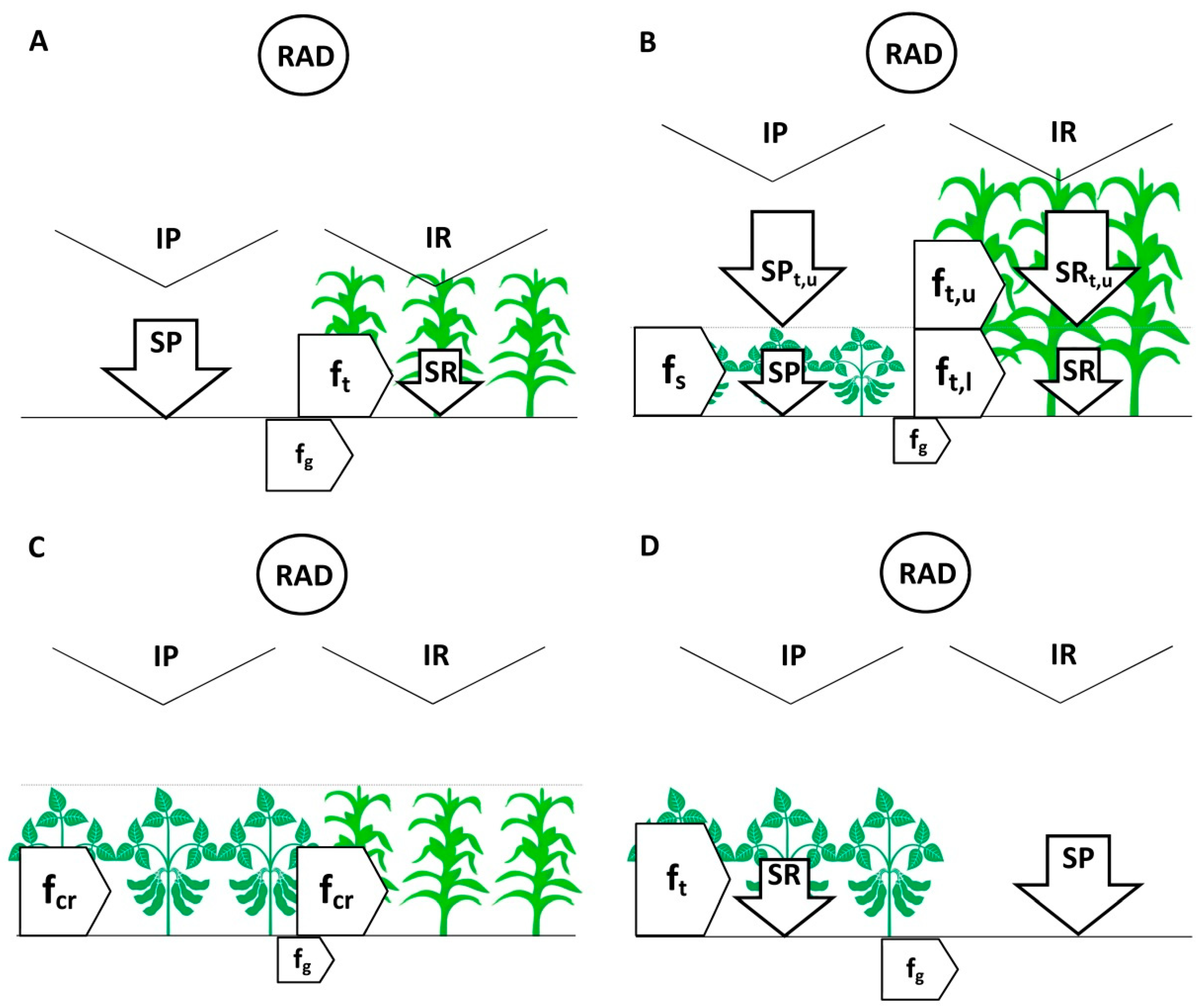
Radiation distribution in strip-crop cultivation scenarios. (A) First crop (main) is single, (B) intercropping, main crop is taller, (C) intercropping, crops are of equal height, (D) second crop (companion) is single. RAD, incoming radiation. See Table 1 for the description of the other symbols.
Figure 3.
Radiation distribution in strip-crop cultivation scenarios. (A) First crop (main) is single, (B) intercropping, main crop is taller, (C) intercropping, crops are of equal height, (D) second crop (companion) is single. RAD, incoming radiation. See Table 1 for the description of the other symbols.

Figure 4.
(A) Strip intercrop MS simulated with SWAP 2×1D, (B) monocropping maize (scenario M), and (C) monocropping soybean (scenario S), simulated with SWAP 1D. MLAI is the maximum LAI in the season.
Figure 4.
(A) Strip intercrop MS simulated with SWAP 2×1D, (B) monocropping maize (scenario M), and (C) monocropping soybean (scenario S), simulated with SWAP 1D. MLAI is the maximum LAI in the season.

Figure 5.
(A) LAI of intercropped maize (MS) and monocrop (M), (B) intercropped soybean LAI (MS) and monocrop (S), (C) fraction of the radiation interception by plants (ft) and (D) fraction of soil radiation interception (fg).
Figure 5.
(A) LAI of intercropped maize (MS) and monocrop (M), (B) intercropped soybean LAI (MS) and monocrop (S), (C) fraction of the radiation interception by plants (ft) and (D) fraction of soil radiation interception (fg).

Figure 6.
(A) and (B) Maize and soybean daily transpiration rates (Ta), and (C) and (D) soil evaporation rates (Ea).
Figure 6.
(A) and (B) Maize and soybean daily transpiration rates (Ta), and (C) and (D) soil evaporation rates (Ea).

Figure 7.
Soil lateral flux (QL) between soil strips and average minimum hydraulic conductivity (Kmin) from day number 0 to 100 (A) and from 100 to 200 (B). Horizontal bars over the graphs indicate the type and period of cultivation. // means a break in the vertical axis of QL from −1.0 to −3.5 cm d−1. Indicated points in the graphs are (Day,QL) and [Day,Kmin]. Positive values of QL indicate that water flows from the soil under soybean towards the soil under maize.

Figure 8.
Soil water content (θ) in soil profile of maize and soybean simulated with (solid lines) and without (dashed lines) soil water lateral flux on days 48 (A) and 71 (B).
Figure 8.
Soil water content (θ) in soil profile of maize and soybean simulated with (solid lines) and without (dashed lines) soil water lateral flux on days 48 (A) and 71 (B).


Table 1.
List of symbols with description, units, and first equation in which they occur.
| Symbol | Description | Equation | Unit |
|---|---|---|---|
| Radiation | |||
| ft | Fraction of radiation intercepted by a strip-canopy | (1) | - |
| fh | Fraction of radiation intercepted by a homogeneous type canopy | (2) | - |
| fc | Fraction of radiation intercepted by a compressed type canopy | (3) | |
| LAI | Leaf area index over the whole intercropped area | - | m2 m−2 |
| LAIc | Leaf area index of a compressed canopy | (4) | m2 m−2 |
| MLAIi | Maximum leaf area index over the whole intercropped area | m2 m−2 | |
| MLAIm | Maximum leaf area index over the whole monocropping area | m2 m−2 | |
| w | Factor expressing the relative homogeneous and compressed contribution to the canopy radiation interception model | (5) | - |
| SR | Fraction of radiation reaching the soil under the strip | (6) | - |
| SP | Fraction of radiation reaching the soil path | (7) | - |
| IP | View factor over the soil path | (8) | - |
| IR | View factor over the strip | (9) | - |
| LAIt,u | Leaf area index of the taller plants in the upper canopy layer | (10) | m2 m−2 |
| LAIt,l | Leaf area index of the taller plants in the lower canopy layer | (11) | m2 m−2 |
| LAIs,c | Leaf area index compressed of the shorter plant | ||
| ft,l | Fraction of radiation interception by the taller plant in the lower layer | (13) | - |
| ft,u | Fraction of radiation interception by the taller plant in the upper layer | (1)–(9) | - |
| SRt,u | Fraction of radiation transmitted through the upper part of the taller plants | (14) | - |
| fs | Fraction of radiation intercepted by the shorter plants | (15) | - |
| SPt,u | Fraction of radiation transmitted between and through the taller plant to the path | (16) | - |
| fcr | Fraction of radiation intercepted by strip plants with the same height | (17) | - |
| fg | Fraction of radiation intercepted by the soil | (18) | - |
| ft1 | Total fraction of the radiation interception by one plant species in the intercropping | (18) | - |
| ft2 | Total fraction of the radiation interception by a second plant species in the intercropping | (18) | - |
| kcf | Light extinction coefficient | - | - |
| ks | Light extinction coefficient of the shorter plant | - | - |
| kt | Light extinction coefficient of the shorter plant | - | - |
| kcr | Light extinction coefficient of a intercropped plant | - | - |
| R | Strip width | - | cm |
| P | Path width | - | cm |
| Ht | Plant height of the taller plant in the intercrop | - | cm |
| Hs | Plant height of the shorter plant in the intercrop | - | cm |
| Rt | Strip width of the taller plant in the intercrop | - | cm |
| Pt | Path width of the taller plant in the intercrop | - | cm |
| Rs | Strip width of the shorter plant in the intercrop | - | cm |
| Ps | Path width of the shorter plant in the intercrop | - | cm |
| Rcr | Strip width of a intercropped plant | - | cm |
| Pcr | Path width of a intercropped plant | - | cm |
| Water flux | |||
| Tp,i | Potential transpiration of each plant separately | (19) | cm |
| Ep | Potential evaporation | (20) | cm |
| Wc | Fraction of the day during which the canopy is wet | (19) | - |
| ∆v | Slope of the saturated vapor pressure-temperature curve | (19), (20) | kPa °C−1 |
| λw | Latent heat of vaporization | (19), (20) | kJ kg−1 |
| Rn | Net radiation at the canopy surface | (19), (20) | J m−2 d−1 |
| G | Soil heat flux density | (19), (20) | J m−2 d−1 |
| p1 | Unit conversion value | (19), (20) | s d−1 |
| ρa | Air density | (19), (20) | kg m−3 |
| Ca | Heat capacity of the moist air | (19), (20) | J kg−1 °C−1 |
| esat | Saturation vapor pressure | (19), (20) | kPa |
| ea | Actual vapor pressure | (19), (20) | kPa |
| γa | Psychrometric constant | (19), (20) | kPa °C−1 |
| ra,c,i | Aerodynamic resistance of the plant canopy | (21) | s m−1 |
| ra,g | Aerodynamic resistance of the soil | (22) | s m−1 |
| rs,min,i | Minimum stomatal resistance | (19) | s m−1 |
| LAIeff | Effective leaf area index | (19) | |
| rsoil | Soil resistance of a wet soil | (20) | s m−1 |
| Pin,i | Water interception by the plant canopy | (23) | cm |
| Pgross | Gross precipitation | (23) | cm d−1 |
| a | Empirical coefficient for the precipitation interception | (23) | |
| ql,d | Lateral Darcian water flux between soil compartments | (24) | cm d−1 |
| Kmin | Hydraulic conductivity of the driest same-level soil compartment | (24) | cm d−1 |
| Dn | Distance between the centers of two neighboring strips of different plant species | (24), (25) | cm |
| h1, h2 | Soil pressure head | (24) | cm |
| qlim,d | Limiting lateral flux per compartment | (25) | cm d−1 |
| ∆θ | Difference in soil water content of two same-level soil compartments | (25) | |
| qd | Lateral flux per soil compartment limited by qlim | (26) | cm d−1 |
| Bc,i | Plant-ground coverage fraction | (27), (31) | cm2 cm−2 |
| QL | Total lateral flux of the soil profile | (27) | cm d−1 |
| Water balance | |||
| Pa | Precipitation | (29), (30) | cm |
| Ta | Plant transpiration | (29), (30) | cm |
| Ea | Soil evaporation | (29), (30) | cm |
| Qb | Bottom flux | (29), (30) | cm |
| ∆S1 | Variation of soil water storage in soil-plant module 1 | (29), (31) | cm |
| ∆S2 | Variation of soil water storage in soil-plant module 2 | (30), (31) | cm |
| ∆Sin | Variation of soil water storage for the intercropping | (30), (31) | cm |
| Sensitivity analysis | |||
| η | Relative partial sensitivity index | (32) | - |
| Vf | Default value of a generic output variable | (32) | |
| Vs | New value of the output variable after a selected parameter was changed | (32) | |
| Vr | Reference value of the output variables evaluated in the sensitivity analysis | (32) | |
| p | General representation for parameter | (32) | |
| ∆p | Change in the parameter values in the sensitivity analysis | (32) | |
| Cref | Canopy reflection coefficient | - | |
| RLAI | Maximum relative increase in LAI | m2 m−2 d−1 | |
| kdif | Extinction coefficient for diffuse light | - | |
| kdir | Extinction coefficient for direct light | - | |
| Өr | Saturated soil water content | cm3 cm−3 | |
| Өs | Residual soil water content | cm3 cm−3 | |
| α | Soil water retention curve parameter | cm−1 | |
| n | Soil water retention curve parameter | - | |
| Ks | Saturated hydraulic conductivity | cm d−1 | |
| l | Soil hydraulic conductivity exponent | - |
Table 2.
Overview of the simulated scenarios.
| Scenario | Model | Description | Objective |
|---|---|---|---|
| Maize–soybean (MS) intercropping | SWAP 2×1D | Strip intercropping MS (Figure 4A). Soybean is sown approximately 50 days after maize. | Application of SWAP 2×1D to a strip intercropping system |
| Maize monocropping (M) | SWAP 1D | Monocropping cultivation of maize (Figure 4B) | To compare the water balance outcomes of monocropping to the intercropping scenario. |
| soybean monocropping (B) | SWAP 1D | Monocropping cultivation of soybean (Figure 4C) | To compare the water balance outcomes of monocropping to the intercropping scenario. |
Table 3.
Main plant parameters used in the simulation scenarios for maize and soybean (MS), maize (M) and soybean (S).
Table 3.
Main plant parameters used in the simulation scenarios for maize and soybean (MS), maize (M) and soybean (S).
| Description | Parameter | Maize | Soybean | Unit |
|---|---|---|---|---|
| Plant maximum height | Hmax | 200 | 80 | cm |
| Reflection coefficient, Albedo | Cref | 0.20 | 0.23 | - |
| Minimum canopy resistance | RSC | 131 | 70 | s m−1 |
| Temperature sum from emergence to anthesis | Tsum,ea | 1000 | - | °C |
| Temperature sum from anthesis to maturity | Tsum,am | 1150 | - | °C |
| Maximum CO2 assimilation rate | Amax,d | 35 | 37 | kg ha−1 d−1 |
| Maximum relative increase in LAI | RLAI | 0.012 | 0.010 | m2 m2 |
| Extinction coefficient for diffuse visible light | kdif | 0.60 | 0.80 | - |
| Extinction coefficient for direct visible light | kdir | 0.75 | 0.80 | - |
| Light use efficiency | eff | 0.45 | 0.40 | kg CO2 J−1 |
| Assimilates conversion efficiency into leaves | Cvl | 0.68 | 0.72 | kg kg−1 |
| Assimilates conversion efficiency into storage organs | Cvo | 0.67 | 0.68 | kg kg−1 |
| Assimilates conversion efficiency into roots | Cvr | 0.29 | 0.72 | kg kg−1 |
| Assimilates conversion efficiency into stems | Cvs | 0.66 | 0.69 | kg kg−1 |
| Relative increase in respiration rate with temperature | Rit | 2.00 | 2.00 | kg CH2O kg−1 d−1 |
| Relative maintenance respiration rate of leaves | Rml | 0.03 | 0.03 | kg CH2O kg−1 d−1 |
| Relative maintenance respiration rate of storage organs | Rmo | 0.01 | 0.017 | kg CH2O kg−1 d−1 |
| Relative maintenance respiration rate of roots | Rmr | 0.015 | 0.010 | kg CH2O kg−1 d−1 |
| Relative maintenance respiration rate of stems | Rms | 0.015 | 0.015 | kg CH2O kg−1 d−1 |
| Maximum relative death rate of leaves due to water stress | Pdl | 0.03 | 0.03 | d−1 |
| Critical pressure heads according to Feddes [33] | h1 | −10.0 | −15.0 | cm |
| h2u | −25.0 | −30.0 | cm | |
| h2l | −25.0 | −30.0 | cm | |
| h3h | −400.0 | −750.0 | cm | |
| h3l | −500.0 | −2000.0 | cm | |
| h4 | −10000.0 | −8000.0 | cm | |
| Interception coefficient, corresponding to maximum interception amount | a | 0.25 | 0.25 | cm |
| Maximum daily increase in rooting depth | Rrd,i | 2.20 | 1.2 | cm d−1 |
| Maximum root depth | Rd,m | 100 | 100 | cm |
| Below ground plant coverage | Bc | 0.5 | 0.5 | - |
Table 4.
Main soil parameters used in the simulation scenarios.
| Description | Parameter | Value | Unit |
|---|---|---|---|
| Soil resistance of wet soil | rsoil | 230 | s m−1 |
| Soil evaporation coefficient of Black | Cbk | 0.45 | cm1/2 |
| Residual water content | Өr | 0.13 | cm3 cm−3 |
| Saturated water content | Өs | 0.37 | cm3 cm−3 |
| Parameter alfa of the water retention curve | α | 0.04 | cm−1 |
| Parameter n of the water retention curve | n | 1.59 | - |
| Exponent in the hydraulic conductivity function | l | 1.2 | - |
| Hydraulic conductivity at saturated conditions | Ksat | 26 | cm d−1 |
Table 5.
Water balance components for intercropping MS and monocropping maize and soybean: ∆S, water storage change; P, precipitation; Qb, bottom flux; Pi, canopy water interception; Ta, actual transpiration; Ea, actual evaporation; ETa and ETP, actual and potential evapotranspiration, respectively; Tp, potential transpiration; Ep, potential evaporation.
| Water Balance Components | SWAP 1D | SWAP 2×1D | ||
|---|---|---|---|---|
| (cm) | Maize | Soybean | MS 1D Average | MS |
| Actual | ||||
| ∆S | 4.1 | 1.1 | 2.6 | 1.1 |
| Pa | 47.7 | 47.7 | 47.7 | 47.7 |
| Pi | −2.7 | −1.0 | −1.9 | −1.6 |
| ETa | −40.8 | −37.2 | −39.0 | −41.6 |
| Ta | −24.6 | −17.7 | −21.1 | −25.4 |
| Ea | −16.2 | −19.5 | −17.9 | −16.1 |
| Qb | −0.1 | −8.3 | −4.2 | −3.5 |
| Potential | ||||
| ETp | 74.3 | 75.0 | 74.7 | 73.2 |
| Tp | 24.6 | 24.2 | 24.4 | 31.4 |
| Ep | 49.7 | 50.8 | 50.3 | 41.8 |
Table 6.
Relative partial sensitivity index η of soil and atmospheric fluxes for plant and soil parameters predicted by the SWAP 2×1D model.
Table 6.
Relative partial sensitivity index η of soil and atmospheric fluxes for plant and soil parameters predicted by the SWAP 2×1D model.
| Parameter | η | |||||||||||||
|---|---|---|---|---|---|---|---|---|---|---|---|---|---|---|
| Maize | Soybean | |||||||||||||
| ∑ft | Tp | Ta | Ep | Ea | QL | Qb | ∑ft | Tp | Ta | Ep | Ea | QL | Qb | |
| Maize | ||||||||||||||
| RUE | 0.17 | 0.63 | −0.11 | 0.00 | −0.21 | −0.21 | −0.42 | 0.00 | 0.00 | 0.00 | −0.42 | −0.11 | 0.21 | 0.00 |
| Cref | 0.01 | −1.16 | 1.05 | 0.00 | 0.00 | 1.05 | 2.21 | −0.01 | 0.00 | 0.00 | 0.00 | 0.00 | −1.05 | −1.16 |
| RLAI | 0.27 | 1.26 | −2.00 | −0.01 | −0.42 | −2.31 | −4.62 | −0.01 | 0.00 | 0.11 | −0.74 | −0.21 | 2.31 | 2.00 |
| kdif | 0.19 | 0.53 | 0.00 | 0.00 | −0.42 | −0.42 | −0.95 | −0.07 | −0.21 | 0.11 | −0.42 | −0.11 | 0.42 | 0.21 |
| kdir | 0.40 | 1.26 | 0.42 | −0.01 | −0.53 | −0.11 | −0.11 | −0.06 | −0.21 | 0.11 | −0.84 | −0.21 | 0.11 | −0.32 |
| Soil | ||||||||||||||
| Өr | 0.00 | 0.00 | 0.32 | 0.00 | 0.11 | 0.74 | 1.47 | −0.18 | −0.42 | 0.63 | 0.21 | −0.11 | −0.74 | −1.58 |
| Өs | 0.01 | 0.00 | 5.78 | 0.00 | 1.26 | 7.04 | 14.18 | 0.09 | −0.32 | 0.53 | 0.11 | 1.05 | −7.04 | −7.25 |
| a | −0.03 | −0.11 | −1.16 | 0.00 | 0.00 | −0.74 | −1.47 | −0.12 | −0.32 | 0.42 | 0.21 | 0.00 | 0.74 | 0.53 |
| n | 0.00 | 0.00 | −1.37 | 0.00 | −0.42 | −0.53 | −1.16 | −0.16 | −0.32 | 0.63 | 0.21 | −0.21 | 0.53 | −0.21 |
| Ks | 0.00 | 0.00 | 1.47 | 0.00 | 0.11 | 1.79 | 3.68 | 0.01 | 0.00 | 0.00 | −0.11 | 0.00 | −1.79 | −2.31 |
| l | 0.00 | −0.11 | −0.21 | 0.00 | −0.11 | −0.21 | −0.42 | 0.02 | 0.00 | 0.00 | 0.00 | 0.00 | 0.21 | 0.32 |
Note: Output variable: ∑ft, the sum of daily plant interception fractions; Tp and Ta, potential and actual transpiration rates; Ep and Ea, potential and actual evaporation rates; QL-in, lateral influx; Qb, bottom flux. Parameter: RUE, radiation use efficiency; Cref, reflection coefficient (Albedo); RLAI, maximum relative increase in LAI; kdif and kdir, extinction coefficients for diffuse and direct light, respectively; Өr and Өs, the residual and saturated soil moistures, a and n, retention curve parameters, l, soil hydraulic conductivity parameter, and Ks, the saturated hydraulic conductivity.
© 2019 by the authors. Licensee MDPI, Basel, Switzerland. This article is an open access article distributed under the terms and conditions of the Creative Commons Attribution (CC BY) license (http://creativecommons.org/licenses/by/4.0/).
Share and Cite
MDPI and ACS Style
Pinto, V.M.; van Dam, J.C.; de Jong van Lier, Q.; Reichardt, K. Intercropping Simulation Using the SWAP Model: Development of a 2×1D Algorithm. Agriculture 2019, 9, 126. https://0-doi-org.brum.beds.ac.uk/10.3390/agriculture9060126
AMA Style
Pinto VM, van Dam JC, de Jong van Lier Q, Reichardt K. Intercropping Simulation Using the SWAP Model: Development of a 2×1D Algorithm. Agriculture. 2019; 9(6):126. https://0-doi-org.brum.beds.ac.uk/10.3390/agriculture9060126
Chicago/Turabian StylePinto, Victor Meriguetti, Jos C. van Dam, Quirijn de Jong van Lier, and Klaus Reichardt. 2019. "Intercropping Simulation Using the SWAP Model: Development of a 2×1D Algorithm" Agriculture 9, no. 6: 126. https://0-doi-org.brum.beds.ac.uk/10.3390/agriculture9060126
Note that from the first issue of 2016, this journal uses article numbers instead of page numbers. See further details here.