
Critique on Ecological Methodologies Used in Water Quality Studies and Coastal Management: A Review

Laboratory of Environmental Quality and Geospatial Applications, Department of Marine Sciences, University of the Aegean, GR-81100 Mytilene, Lesvos, Greece
J. Mar. Sci. Eng. 2022, 10(5), 701; https://0-doi-org.brum.beds.ac.uk/10.3390/jmse10050701
Submission received: 1 March 2022
/
Revised: 12 May 2022
/
Accepted: 12 May 2022
/
Published: 20 May 2022
(This article belongs to the Special Issue Decision Support Systems and Tools in Coastal Areas)
Abstract
:The subject of ecology is the understanding of the relations among living organisms and their interactions with the abiotic environment. The need to quantify ecological phenomena requires the development of mathematical tools, including ecological indices, statistical procedures and simulation models. Some of these tools have been found to be convenient by many scientists and policy makers in related scientific disciplines to express marine pollution levels, marine water quality and future trends; they have, therefore, been adopted in coastal management methodologies and practices. In the present work, a number of ecological tools are reviewed regarding their relevance to supporting water quality studies, as well as their suitability to be included in the toolkit of coastal management practices. Their problems and weaknesses, together with the science–policy misconnection, are discussed.
1. Introduction
The main objective of ecology is the study of the relations among organisms as well as their relation with the environment that they live in. Ecology is, therefore, a multidimensional approach embracing many different scientific disciplines; in addition to scientific fields, such as physics, chemistry and geology, ecology also includes diverse fields within the biological sciences, such as taxonomy, physiology, population dynamics, population genetics and evolutionary biology [1]. Ecological research can be classified into two main clusters: the qualitative approach and the quantitative assessment of particular phenomena. The qualitative aspect refers to the understanding of the life cycles of organisms, the type of relation between two or more organisms, their trophic behavior, their survival mechanisms and the factors affecting the population dynamics of some species, to mention a few. The need for quantitative knowledge of ecological processes increases at a more mature stage of ecological research, aiming at the evaluation of the significance of certain ecological issues in “terms of numbers”. The most common quantitative ecological methods focus on the assessment of species abundance, species richness, species associations, biomass, energy flow and nutrient cycling. The tendency of ecologists to formulate and solve issues by mathematical reasoning using a wide variety of mathematical tools is a common practice nowadays [2].
A few decades ago, environmental concerns were politicized. Due to this intense political interest in marine environmental issues, ecological information has been used as a tool in marine water quality and ecosystem health issues. According to De Jong [3]: “this relationship has been strengthened and thus, the potentials for the transfer of scientific information from science to politics and requests from politics to science” leading to “policy research connectivity”. In this way, various ecological measures, inter alia, species diversity, biomass and energy flow, gained environmental significance. Diversity indices are a good example—as early as 1968, Wilhm and Dorris [4] suggested that some biological parameters, mainly Shannon’s diversity index, could be used for water quality studies [4]. Meanwhile, many more ecological indices have become popular as environmental indicators. However, when the suitability of biotic diversity and similarity indices was reviewed by Washington [5], the findings were rather poor. Washington, after having examined eighteen diversity indices, nineteen biotic indices and five similarity indices, concluded that most of them were unsuitable for use in water pollution studies. However, it was at the Rio Summit in 1992 that diversity, although it was not an exclusive subject for ecologists and environmental activists, “became a matter of preoccupation and political debate” [6]. Many people and institutions outside the ecological community feel that biodiversity protection is a key issue for a sustainable planet. This is why diversity indices, together with other ecological indices, became the “Holy Grail” in environmental policy and decision making.
During the last three decades, ecological indicators have been highly recommended in legal documents, such as the European Union Directives [7,8] and International Conventions for the Protection of the Marine Environment [9,10,11]. A good example is the European Union Directives already mentioned above, namely the Directive for Water Policy [7] and the Directive for Marine Strategy [8]. The use of ecological indicators and the development of new ones is encouraged, as the main objective of those Directives is “good environmental status”, which is defined as “the environmental status of marine waters where these provide ecologically diverse and dynamic oceans and seas which are clean, healthy and productive within their intrinsic conditions…”. In spite of the objectivity of the indicators, it is not possible to gain a good understanding of the health of an ecosystem just by one or a few numbers. Reservations have already been expressed [12] regarding regulatory decisions to be made in the absence of understanding an ecosystem’s functioning. Although this skepticism has been expressed in connection with toxicity aspects, it may be considered as a general principle in policymaking. Beyond the ecological indicators, statistical methods, especially multivariate analysis and simulation modeling, also play an important role in ecological reasoning, assessment and prediction.
The use of mathematical procedures in ecology is different when addressing an ecological issue, being useful for hypothesis generation and understanding ecological phenomena, and are different when used as an “objective tool” for policy making, where precision and reliability are required. In pure ecological terms, the objectives of a quantitative ecological approach are: (a) to condense large data sets into a few numbers or even a graph, (b) to find any possible trends and (c) to use the results as a basis for further hypothesis generation. However, in terms of policy, the outcomes of data analysis can be used for policy purposes, sometimes being included in environmental laws and regulations. In spite of the research–policy connectivity, discrepancies often arise in the interface between science and policy [13]. These discrepancies may be due to a number of factors, such as problem complexity, disagreements among scientists and different scaling between scientific and political processes. An additional factor that has not received enough attention so far, in the author’s opinion, is the uncertainty of the scientific outcome due to physical uncertainty, as well as to the uncertainty carried through scientific information processing. The latter is the objective of the current work, which aims to evaluate the methodological limitations in ecological studies used for environmental regulatory purposes.
The objective of the present work is to evaluate quantitative ecological methods from two points of view. First, to determine whether they are suitable for marine water quality studies by considering their weak points. Second, to assess whether they are resilient enough to cope with a system’s uncertainty, taking into account the complexity of ecosystems, together with data availability, as sets of data may be limited in terms of variables and data points. In addition, certain variables of primary importance are rarely measured due to experimental and/or sampling or cost constraints. Limited data availability and a lack of key variables increase methodological error and bias in some data analysis procedures, adding to the uncertainty of the outcome.
2. Data Collection and Selection of Variables
2.1. Sampling Design Considerations
The difficulties regarding the validity of data start from sampling. The natural environment, terrestrial or marine, is not homogenous. A common phenomenon in the marine environment is what is known as “patchiness”, that is, many organisms are grouped together in specific patterns, forming clusters. Patchiness is very common in planktonic communities: one of the reasons is Langmuir circulation, as plankton assemblages are swept towards the edges of Langmuir cells. It seems that other mechanisms favoring patchiness also exist, but they are not yet known with certainty. These are questions beyond the objective of the current article regarding the survival of planktonic organisms [14]. Although the transportation of planktonic organisms mainly depends on the currents, fishes are active swimmers, able to avoid unfavorable conditions and search for suitable breeding and feeding grounds. Many individuals of the same fish species form clusters that are groups of fishes known as schools, a mechanism that also gives fish a patchy distribution pattern. Significant inhomogeneity also occurs in benthic biota: typical cases are bed formations of seaweeds, as well as beds of mussels. It is obvious that, if random sampling is applied in an area that shows significant heterogeneity, the variance of the measured variables would be rather high. However, the majority of the sampling schemes applied routinely follow a random sampling strategy. Some efforts have been made to develop sampling designs to optimize sampling site selection in coastal marine environments. In the Island of Lesvos, Greece, a grid of 34 sampling sites was organized along the Strait of Lesvos and water samples were collected for measuring the chlα concentrations [15]. The stations were reallocated into three groups based on the standard error of the chlα measurements. Variograms were used for station reallocation by estimating the heterogeneity and anisotropy of the chlα distribution pattern. The methodology proposed an optimized sampling design by eliminating the number of stations and maximizing information at the spatial level. Although stratified sampling and optimal sampling are known in the literature [16,17,18], applications of this methodology are limited in marine ecological studies, especially in terms of chlα distributions. One of the reasons may be the relatively high mathematical complexion, especially regarding the spatial methodology. Another reason is related to the need to perform a number of preliminary samplings in order to have enough data for optimizing the sampling sites. Many projects are run in the form of surveys, a fact that limits the possibility of repeated samplings and, therefore, does not give the experimenters a chance to elaborate a comprehensive design for the study area; in these cases, sampling design is based only on the personal experience of the researcher in the area. A marine monitoring program in the Bohai Sea (China) used a network of many sampling sites that were used for optimization [19]. They ended up with two groups of stations (225 and 181) for optimizing operational monitoring, accounting for 46.5% and 37.4% of the original sampling sites, respectively. Furthermore, they found higher reproducibility and efficiency in the optimized system.
Sampling design optimization is absolutely necessary, as, very often, plankton patchiness appears in both marine and fresh waters. An attempt has been reported in a lake in Finland; the researchers tried to obtain a number of samples in order to obtain an estimate of the representativeness of discrete chlα measurements [20]. Using a flow-through fluorimetric device for chlα concentration measurements, the work aimed: (a) to gain an estimate of the spatial representativeness of discrete sampling and (b) to assess the effect of sample size on both the mean chlα concentration and the observed proportion of variance. The authors suggested that it is risky to generalize the chlα distribution based on a small number of samples, a usual practice in marine monitoring; the low representativeness of the sampling sites was confirmed by the authors during their sampling effort. It has to be mentioned that marine monitoring is not an area of academic research, but collection of information regarding selected variables used for coastal management and decision making.
2.2. Sampling: Some Delicate Issues
It is generally difficult, during a sampling procedure, to judge whether the data sets formed are reliable enough or of limited value. The usual problems reducing sample validity are: (a) the scale of investigation, (b) the inaccessibility of habitats, especially when large depths or distance from the coast are involved, (c) the degree of familiarity of the particular biota sampled and (d) species richness, which is strictly connected to the sample size. When a group of marine organisms is studied, for example, phytoplankton communities, there is always an assumption that usually is not even mentioned: all the classified species are not “equivalent” in a number of ways. Species differ in their functional role within the ecosystem. In addition, the size of the individuals makes them differ in their behavioral and metabolic activities. The first assumption in diversity measurement is that all species are of equal size [6]. Differences in size among individuals make them differ in their behavioral and metabolic activities. Cell size, for example, is a major phytoplanktonic characteristic because it plays a prominent structural role—many physiological and ecological processes tend to escalate with cell size. Production, abundance, nutrient turnover rates and prey–predator aspects are the most important [21]. A cell size gradient has been identified regarding phytoplankton cell size, ranging from nanoplankton (10–103 μm3) and microplankton (103–106 μm3) up to macroplankton (106–109 μm3) [22,23]. Different sizes of phytoplankton cells respond in different ways to environmental perturbations, to nutrient availability and to the presence of organic compounds; organic compounds function either as stimulants or as inhibitors, inducing the loss of certain species in favor of others that can take an advantage. Unfortunately, because of the way that lists of species are set up, significant characteristics of subgroups are “flattened” and valuable information is lost. The consequences of the “species equivalence” assumption does not only affect biodiversity issues, but is also related to the carbon biomass of the cells. The algal cell carbon content is a key point in biomass estimates: chlorophyll concentrations as well as fluorescence responses cannot be used as reliable estimators of phytoplankton biomass [23]. Biomass estimates, however, are the principal variables in ecological modeling. In addition, phytoplankton biomass is currently used for estimates of carbon dioxide assimilation by marine photosynthetic biota in connection with climate change issues.
The classification and enumeration of plankton communities is carried out through the microscopic examination (microscope or stereoscope) of the samples. There are usually common species characterized by high abundance and frequency of occurrence. At the same time, there are species that occur once or twice in the whole sample; that is, they are restricted in numbers and, therefore, they are considered as “rare”. Although the recording of species of high abundance can be assumed, from the viewpoint of statistics, to follow normal or log-normal distribution, the recording of rare species seems to follow the binomial distribution (presence–absence). The overall result is the synthesis of the two distributions; in that case, the log-normal distribution pattern is further skewed to the right; in other words, the overall pattern is actually bimodal, disguising the two distributions [24]. The log-normality raises a number of problems during data analysis, and these problems are discussed later in this article (Section 6: “Statistical considerations”). After all, the absence of a rare planktonic species from the marine environment does not mean that the particular species does not exist. It is a matter of sample size whether a rare species appears under the microscope, and this is not, therefore, a real problem of species existence. The problem arising from the inclusion or non-inclusion of rare species in the sample is not simply a computational problem, but also a problem of great ecological significance. There are researchers [25] maintaining that rare species are artifacts, simply adding noise to statistical approaches and, therefore, should be excluded. Others [26] support the view that rare species are an ecologically significant component of population dynamics and, in any case, they should be taken into account. Rarity is considered more and more as an element of ecological importance regarding biodiversity and productivity-related processes. A study on rare species regarding coastal phytoplankton assemblages was published by Ignatiades and Gotsis-Skretas [27]. Using phytoplankton data collected in the Aegean Sea, Eastern Mediterranean, they found that rare species contributed 6.4% of the total cell abundance, 13.1% of the total species diversity, 21.2% of the total cell volume and 16.6% of the total carbon biomass. Unfortunately, there are only a few studies in marine communities depicting the significant role of rare species. Rare species have been characterized as reservoirs of ecological and genetic diversity [28]. The role of rare species is compensatory, contributing to the stability of the community [26]. Similar views have been expressed through “the insurance theory” [29] responding to disturbance, thereby strengthening the resilience of ecosystem processes.
2.3. Data Collection for Regulatory Policies
Political decisions regarding coastal management require, inter alia, reliable field information referring to coastal marine environmental quality and ecosystem health. Data collection should follow a regular time basis (monthly or seasonal collection of data), with a well-organized sampling design. This systematic observation of the marine environment, which forms the basis of marine environmental assessment regarding water quality and ecosystem health, is known as “monitoring” [30]: “monitoring is a systematic observation of parameters related to a specific problem designed to provide information on the characteristics of the problem and changes with time”. It is, therefore, evident that eco-logical–environmental assessment in marine monitoring is closely linked with policy making [30]. Due to the significance of this information, many international organizations, as well as international conventions, have indicated the mandatory variables that should be monitored. For example, the Mediterranean Monitoring Programme, known as MED POL [31], requires measurements of the sea temperature, pH, transparency, salinity (background variables), nutrients (causal variables), dissolved oxygen and chlorophylls (effect variables). It also requires measurements of the concentration of certain toxic compounds, including petroleum hydrocarbons and some heavy metals, in the water column, sediments and biota [32]. Some of the variables used for marine monitoring according the protocols of international conventions are provided in Table 1.
This way, scientists and policy makers can have a good understanding of the present conditions and they will be able, over time, to observe trends, if there are any. Beyond the monitoring mentioned above “senso stricto”, it is useful to develop ecological models, not so much for forecasting purposes, but for testing different scenarios. It is known that ecological models are more sensitive to rates rather than the state variables mentioned. The most important variables referring to rates are photosynthetic rates, grazing and the decomposition of organic matter by bacteria. The measurement of photosynthetic rates in the marine environment is based on a well-established 14CO2 method [38]. Although there have been data on photosynthetic rates available since the 1950s, the grazing and organic matter decomposition rates are rarely measured. This problem will be further discussed in the section regarding modeling.
3. Βiοindicator Species
As a response to ecosystem complexity, the practice of “indicator species” or bioindicators has been coined. There are many definitions in the literature, all focusing on the assessment of an ecosystem’s quality using a single species (or a small number of species). According to a relatively recent definition [39]: “Bioindicators are living organisms such as plants, planktons, animals and microbes which are utilized to screen the health of the natural ecosystem in the environment. They are used for assessing environmental health and biogeographic changes taking place in the environment”. Siddig et al. [40] provided a definition of bioindicators, connecting their use to environmental monitoring: “Indicator species are used to monitor environmental changes, assess the efficacy of management and provide warning signals for impeding ecological shifts”.
Marine bioindicator species include a wide spectrum of organisms, such as foraminifers, diatoms, dinoflagellates [41], microbes [39], crustaceans, mussels, sea turtles and fish [39,42]. Among the criteria for the selection of bioindicator species are their cosmopolitan distribution, easy sampling, high abundance, easy taxonomic identification and moderate tolerance of pollution [42,43]. Although the idea of using indicator species stems from toxicity experiments, including various types of industrial effluents and heavy metals [44], mainly mercury, cadmium, arsenic, chromium and lead, the fields of application these days have been widened. These fields include climate change, plastic pollution [42,45], petroleum hydrocarbons [46], eutrophication [47] and pesticides [43].
The use of indicator species has become wider over the last few years, not only by ecologists and conservation biologists, but also by environmental practitioners. Siddig et al. [40] presented an interesting review of the plethora of uses of indicator species, covering a 14-year period of bibliographic research. However, despite its popularity, the indicator species approach has been criticized for several reasons. Table 2 presents the benefits and drawbacks of the use of indicator species. Some authors have provided incentives for the use of indicator species in monitoring programs for assessing environmental quality [48]. A positive aspect is related, in most cases, to species of commercial value and, therefore, of economic interest. Although the use of indicator species is encouraged as mandatory in marine monitoring programs, international conventions and the European Union Directives, the multitude of causal interactions makes the interpretation of the results exceedingly difficult. These results may be of some value from an ecological point of view, as they can generate hypotheses for further research, but they are fulfilling managers’ expectations, as managers require simple, accurate and conclusive information, which is often used for environmental practices and regulatory policies. On the other hand, ecologists require an understanding of environmental and ecological processes before suggesting regulatory measures, as they have a better “feeling” of an ecosystem’s complexity. The problem of interfacing between ecologists and policy makers that is the coupling of ecological perspectives with managerial practices has been ongoing for a long time [13,49]. However, another benefit of the use of species indicators is the low cost of data collection. The easy sampling and taxonomic identification was mentioned in the previous paragraph. An additional benefit is their use as legislative mandates. If indicator species are included in international conventions for the protection and governance of the seas [10], such as the Barcelona Convention (BARCON), the North Sea and NE Atlantic Convention (OSPAR) and the Caspian Sea Convention (HELCOM), they cover wide areas and many member states participating in these conventions.
Despite the simplicity and the objectivity of species indicators, there are also drawbacks that reduce their effectiveness. Their prognostic power is limited. If their use is based on presence–absence, the development of an ordinal scale is not possible. This drawback is particularly important within, for example, the European Union (EU) legislation, as most of the EU Directives, such as the Directives on Water Policy (2000/60/EU) and the Marine Strategy Directive (2008/56/EU), require a five-level water quality scale to characterize an ecosystem’s quality (high, good, moderate, poor and bad status). If bioindicators are used in laboratory research, the possible lack of experimental protocols might lead to different results and, therefore, different conclusions [50]. Another point of criticism regarding the use of bioindicators is that they are scale-dependent: a fish species as an indicator is very likely to provide information that will not cover ecosystem aspects concerning, for example, the primary trophic level [51]. In addition, each indicator species has specific habitat requirements that do not necessarily reflect the habitat requirements of other species of the same ecosystem [51]. In other words, the use of one species or a small number of species may be an oversimplification of a complex system. Not all of these drawbacks mean that species indicators are not suitable for management practices. Simply, the information they provide should be assessed in connection with the body of information from physical, chemical and biological variables.

Table 2.
Bioindicator species: benefits and drawbacks from their use in water quality studies.
| Benefits and Drawbacks | References | |
|---|---|---|
| Benefits | ||
| A1 | Used for monitoring environmental quality | [48] |
| A2 | Data collection at a low cost | [52] |
| A3 | Testing of toxic contaminants | [52] |
| A4 | Monitoring synergistic and antagonistic impacts of various pollutants on a species | [39] |
| A5 | Easy identification of the indicator species | [52] |
| A6 | Legislative mandates covering wide areas | [51] |
| Drawbacks | ||
| B1 | Oversimplification of the ecosystem’s complexity | [51] |
| B2 | Sometimes different results leading to different conclusions are likely to be produced | [50] |
| B3 | Spatial and temporal uncertainties | [42] |
| B4 | Ecosystem’s complexity restricts their validity | [53] |
| B5 | Development of an ordinal water quality scale may not be possible | [54] |
| B6 | Bioindicator’s ability is scale-dependent | [51] |
4. Ecological Indices: Are They a Reliable Tool for Coastal Management?
4.1. General Views of Diversity
The family of diversity indices is the most popular among the ecological indices. Diversity, generally speaking, is quantified not only on the basis of the number of species in a collection, but also on the relative abundances of each species in the community. If all species in a community occur with almost the same proportion, then that community is more diverse than another where some of the species show high abundance and the rest are what are known as “rare species”. Many formulas have been proposed in the literature expressing diversity based on different principles or theories [5], but most of them share a common feature: the number of species and their evenness in abundance are introduced in most formulas. These days, there are more than ten different diversity indices routinely used for the marine environment [2,5,32,55]. The concept of diversity was first introduced by Williams in 1943 [56]. A number of diversity indices appeared in the literature over the two decades that followed this publication, but during the first period, they were used exclusively by ecologists in their research to express how variable and rich the ecosystem under study was. Later, some researchers found that there was a relationship between the values of some indices and water quality, characterizing an ecosystem’s health [4,55,57].
Whatever the use of diversity values may be, diversity measurements should obey three assumptions [6]: according to the first assumption, all species are equal. This assumption means that species important for conservation or species that make a disproportionate contribution to the community with special functions or genetic value do not receive special weighting. In this respect, species richness, being the oldest and most fundamental concept in expressing diversity [58], does not seem to be particularly informative as it does not quantify the contribution of each species in the community. According to the second assumption, all individuals are equal: a young, for example, fish “weighs” in the index’s outcome the same as an adult fish of the same species.
Among the ecological indices, the most popular are the diversity indices. There are a plethora of ecological indices to choose as a measure of diversity. Among the diversity indices occurring in the literature, some are popular, whereas others are not routinely used. A problem arises because some popular diversity indices are not the best, especially when used for water quality studies [59]. Beyond the problems arising from the use of diversity indices, researchers should bear in mind some basic criteria when choosing an index. Each ecological or diversity index is highlighting specific aspects of an ecosystem [60]; this means that, when an index is chosen, work objectives and experimental designs should be taken into account. In addition, criteria such as sample size, replication and heterogeneity should also be considered [6].
Indices chosen for coastal and marine water quality should fulfill, as much as possible, a number of criteria [61]. They should be sensitive to environmental conditions (geological, physical, chemical and biological), especially in relation to human activities. They also should be connected with functional aspects of the ecosystem, such as the food web, safety and risks from human activities. In addition, they should provide a basis for international comparisons as much as possible, and they should be easy to measure and interpret. The need for a wider geographical validity of these indices is connected with the fact that marine environmental governance and protection is now under the aegis of international conventions. Examples are the conventions for the Mediterranean Sea (BARCON), the North Sea (OSPAR), the Caspian Sea (HELCOM) and the Wider Caribbean Region (Cartagena Convention). The jurisdiction of these conventions extends over wide geographical areas. The data that are required to support the updating of an index’s values should be obtainable regularly through reliable procedures. At this point, the variables involved in an index used in monitoring schemes are included. The indices should be based on sound scientific theories and be robust enough for their information to be provided to economic models.
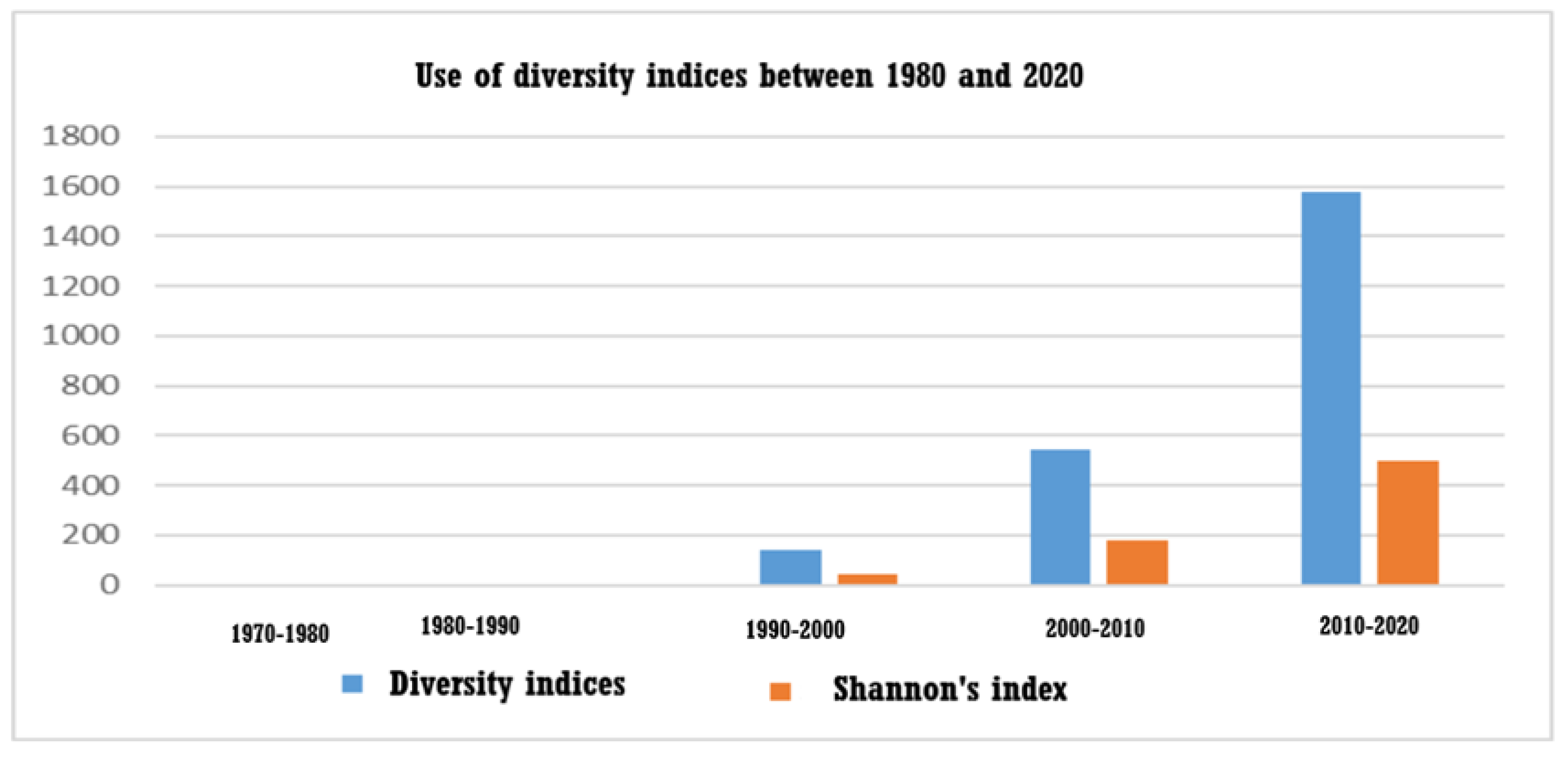
The most comprehensive presentation of diversity indices was presented in 1984 by Washington [5]. The author presented various indices, including Simpson’s Index, based on the probability theory, as well as Odum’s Index (relative to the number of species). Four indices are based on guesses by data fitting (Odum’s Index, Gealson’s Index, Margalef’s Index and Menhinick’s Index). Motomura’s Index is based on the curve-fitting approach and two more indices are based on the information theory (Brillouin’s Index and Shannon’s Index). All indices appearing in the literature obey two assumptions: (a) the whole community is not known, therefore, the calculation of the index is based on samples, being an estimate of the species diversity of the system studied, and (b) the sample is treated as an exact parameter. A bar chart showing the exponential increase in the use of diversity indices in marine studies over the last three decades is presented in Figure 1.
The efficiency of twelve ecological indices in assessing eutrophic levels, that is, their efficiency to discriminate between oligotrophic, mesotrophic and eutrophic conditions, was tested using reference sets of data [59]. These indices included the diversity, abundance, evenness, dominance and biomass of phytoplankton. The results were rather disappointing: three popular indices, fairly often used for water quality studies, that is, Shannon’s Index, Simpson’s Index and Margalef’s Index, seemed to be inappropriate for characterizing eutrophic trends. Other indices, which are less popular, (Menhinick’s index, Kothe’s Index, Species Evenness Index, Species Number Index and the Total Number of Individuals Index), were found to be suitable for assessing the levels of eutrophication. Further work was carried out along that line to test the sensitivity and statistical validity of a number of diversity, evenness and dominant indices to discriminate between oligotrophic and eutrophic conditions [62]. Phytoplankton data were collected from two sampling sites a priori known as oligotrophic and eutrophic, respectively, due to previous work in the area. Using analysis of variance for the detection of differences between the two sampling sites, it was found again that Simpson’s and Shannon’s Indices, widely used in environmental studies for water quality and ecosystem health evaluation, were unsuitable for discriminating between oligotrophy and eutrophication. Regarding Simpson’s Index, it has already been reported [63] that it is neither responsive to environmental impacts nor suitable for the evaluation of an ecosystem’s stability [64]. With the objective of using ecological indices for eutrophication assessment, [62] the following criteria were suggested: the index (a) should be sensitive to nutrient enrichments, (b) should be robust regarding the requirements for statistical analysis and (c) should be powerful in resolving eutrophic levels. Eventually, only four indices fulfilled these criteria: Kothe’s Species Deficit Index, Margalef’s and Gealson’s diversity Indices and Hill’s Index (species number).
The very high popularity of Shannon’s Index and the increasing use of this index in water quality studies have drawn the attention of some ecologists for the further investigation of this index along a eutrophication gradient [65]. Natural and simulated phytoplankton assemblages were studied, which allowed the assessment of the effect of environmental “noise” on an index’s behavior. The results showed that there was considerable unexplained variance in the field data, being sensitive to stochastic processes. The analysis of simulated phytoplankton assemblages using distributions based on the relative abundance indicated that increasing values of Shannon’s Index, in the low range of the eutrophication gradient, were related to increasing species richness, whereas the decreasing index values in the upper range of the eutrophication gradient were due to decreasing evenness. The high variability, together with the non-linearity of Shannon’s Index along a eutrophication gradient, indicates that these measures of diversity are unsuitable for use as tools in water quality monitoring programs. Furthermore, calculations of ecological quality ratios employed by the European Water Framework Directive showed unreliable (non-monotonic) predictions of marine water quality. Water quality assessments required by the European Union Directives, for example, the Water Framework Directive (WFD, 2000/60/EC), assume the monotonicity of the indices as a prerequisite because ecological quality status should be categorized into the five quality classes already mentioned in this article in a rank order. Water quality classification needs robust tools to synthesize information. Reservations about the validity and efficiency of Shannon’s index had already been expressed by Magurran [6]: “despite its popularity, the use of the Shannon Index needs much more justification”. This is a particularly valid comment, as investigations have used it for a long time as their benchmark measure of biological diversity.
4.2. Indices and Marine Environmental Governance
Testing the efficiency of indices for monitoring biodiversity change [66] confirmed what had been already known: “traditional diversity indices are unsuitable for monitoring of biodiversity intactness”. In addition to diversity indices, there are, in the literature, a plethora of indices used to assess an ecosystem’s quality. During the last twenty years, a boom of ecological indicators worldwide has been reported [67]. Some of them have been proposed to be used by International Organizations and Conventions as environmental and ecological quality assessment tools. These International Conventions cover wide geographical areas: the most important are the United Nations (UN) Convention for Biological Diversity, the UN Convention of the Law of the Sea, known as UNCLOS, the European Union Marine Strategy Directive and the US National Ocean Policy [68].
This overabundance of indicators has led to confusion between the concepts of indicators and indices, as they are often treated as synonyms; however, an indicator may be a proxy for something different from what it actually measures [69,70,71]. According to Pinto [71], an index can be considered as a measure of a system’s status, highlighting one or more qualitative and/or quantitative features of the system. However, in the present work, for simplicity reasons, the concept of indicator will also include the term index.
Environmental legislation has also included sections requiring the adoption of methodologies to assess the ecological integrity of both fresh and marine waters. Ecological integrity comprises plankton, zoobenthos, macroalgae, marine angiosperms and fish. Within this framework, an excess of indicators, metrics and evaluation tools was proposed by Borja and Dauer [72]. The main difficulties in developing or selecting an existing index to assess the state of a marine environment are focused on the reliability of the index to be used for policy choices and decision making. This means that the index should be a composite index to describe the dynamics of essential ecological processes, but, at the same time, not be so complex as its physical meaning may be obscured [73].
Indices should be validated, according to Borja and Dauer, according to the following steps [72]: (a) the index should be tested with an independent set of data used already in environmental assessments, (b) it is necessary to set a priori clear-cut criteria and (c) the justification of the results should be performed by personal judgement. At this point, it will be helpful if there is already published work about the issue under study. The validity of an index should be studied by different laboratories in different geographic areas (ecoregions) so that the limits in its applicability can be known. However, the situation described above is rather an ideal picture: very limited evidence exists in the literature regarding reference values (based on pristine conditions), calibration using independent data [74] and the wide geographic application of the index [32]. In addition, the new ecological indices proposed in the literature almost on an everyday basis complicate their validity and make difficult the choice of an index as a tool for policy making purposes.
5. Experimenting: Microcosm Systems
Although coastal management practices can be considered as an “open experiment”, no matter how much relevant information has been collected, there are also laboratory systems, as well as field experimental systems, that significantly contribute to the development of ecological thought. These systems are of relatively small dimensions, with the volume capacity usually ranging between a few liters and a cubic meter, and simple ecosystems set up by researchers are known as microcosm systems [75]. The term microcosm appeared in scientific publications as early as 1963, when they were used to study microbial processes in sewage oxidation ponds [76]. Microcosms also contribute to the understanding of chemical cycles, eutrophication [75,77], the role of limiting factors [78], diversity studies [79], stress and toxicity [80] and climate change [81], but they also contribute significantly to the development of ecological thought [82]. The fields of application of microcosm systems are presented in Table 3.
Microcosm systems can be used as models for generating and testing ecological community theories. Furthermore, they can provide to scientists, as well as policy makers, useful evidence regarding possible environmental decisions. However, the most important advantage of the use of microcosms is their contribution to the understanding of processes and biological mechanisms that cannot be evaluated under field conditions, that is, hazards from toxic compounds [92,93]. The toxic compounds studied in microcosms include petroleum hydrocarbons, insecticides, dispersants, heavy metals, halogenated hydrocarbons, PCBs, dredging spoils and industrial effluents. These days, various emerging pollutants could be added to the list.
Experiments based on single species, although they provide valuable information at biochemical and physiological levels, are inadequate to illustrate effects, processes and mechanisms at the community level. On the other hand, there are also a number of advantages regarding statistical power during the data-processing phase, speed of data analysis because of standard experimental designs, controlled conditions, possible reproducibility among different laboratories and lower cost compared to field studies [12]. There has been skepticism regarding the suitability of single species in toxicity testing [79,94]; the possibility of over or underestimates of toxicity levels to aquatic communities is always a possible outcome due to the fact that single species, no matter how careful and successful their choice may be, cannot efficiently reflect the impact at the community level. The advantages and disadvantages of the use of microcosms are presented in Table 4. There are two types of laboratory microcosms depending on the setting up of the initial community: standardized and natural microcosm systems. In standardized microcosms, the addition of species (usually microalgae and small invertebrates) is carried out according to protocols [95]. On the contrary, natural microcosms are initialized by using natural communities [81]. This type of microcosm is more comparable to the natural environment from where the inoculum comes, although the replicability of aquatic microcosm test systems is generally low. The reproducibility of multispecies experiments involves both precision and accuracy [96]; the number of factors and the duration of the experiment increase the variability of the measured parameters. Due to this constraint, the duration of a microcosm experiment rarely exceeds a period of one month and is usually shorter than that [80,97].
Repeatability is, therefore, rarely examined in microcosms [96]. Another problem regarding the loss of diversity and nutrient exhaustion has been a subject of research [97]. The exhaustion of dissolved nutrients during the experiment leads to the depletion of intercellular nutrient concentrations and this in turn affects the growth of zooplankton. Miller et al. [97] introduced nutrient pulses to microcosms, repeated every three days during their experiment. This type of handling induced greater copepod population densities, increased phytoplankton biomass and allowed the dominance of centric diatoms. Although this experimental approach appears promising, it is a drastic intervention on the design of the experiment and seems to introduce further variability. These limitations restrict the amplitude of data interpretation and primarily provide qualitative information regarding aspects of ecosystem phenomena, rather than endpoints that can be extrapolated directly to the natural environment. In [12], the authors expressed strong reservations regarding the use of the results from microcosm experiments for regulatory decisions, as there are many reasons why these experiments cannot predict effects that will be displayed in natural environments.
Table 4.
Advantages and limitations using laboratory aquatic microcosm systems.
| Advantages–Limitations | References | |
|---|---|---|
| STANDARDIZED AQUATIC MICROCOSMS | ||
| Advantages | ||
| A1 | Experimental replicability | [12,96,98] |
| A2 | No taxonomic uncertainties | [99] |
| A3 | Preformatted statistical analysis | [100] |
| A4 | Controlled degree of complexity | [12] |
| A5 | Species of known physio–ecological characteristics | [92] |
| Limitations | ||
| L1 | Limited number of trophic levels | [75,97] |
| L2 | Standardization cannot include regional or temporal differences | [93] |
| NATURAL AQUATC MICROCOSMS | ||
| Advantages | ||
| A1 | Initial community compatible with the natural environment | [75] |
| A2 | Shelf organization of the community | [75] |
| Limitations | ||
| L1 | Limited number of trophic levels | [75,97] |
| L2 | Limited repeatability | [96] |
| L3 | Uncontrolled degree of complexity | [97] |
| L4 | Unexpected mortality | [92] |
Despite the shortcomings mentioned above, it is interesting to note that the use of microcosms for modeling and simulating ecological processes has obvious advantages. They can provide a good background for describing the dynamics of a “model” of the natural system without the uncertainty of the real world and also provide to the experimenter a chance to test “what if” hypotheses by changing temperatures and nutrient levels (nutrient enrichment), or by adding toxic compounds and alien species to the system. They can be a useful tool in marine environmental assessments, provided that the system’s limitations are well understood.
6. Statistical Considerations
6.1. Assumptions and Drawbacks
Statistical methodology is widely used in ecological research and water quality studies. The current ecological research emphasizes the importance of sampling and statistical design that permit hypotheses to be isolated and tested [101]. However, it seems to be the weakest among the available quantitative tools. This is partly due to the misapplication of statistical models in fieldwork. Ecological statistics is a fast-growing field of statistical applications and it is beyond the limits of this work to deal with this field in detail. This article will be limited to a number of cases where methodological weaknesses can lead to erroneous interpretations and mislead policy makers. The problem starts from the fact that most of the statistical methods, at least the most powerful, have been designed for testing the results of laboratory experiments. Laboratory work can be organized within strict limits and the validity of the assumptions is known (or can be known) in advance [102,103,104].
When designing experiments, there are three possible sources introducing inaccuracies and errors [103]: (a) the “noise” of the system expressed in terms of statistical parameters as experimental error. The error during statistical procedures, derived from field data collected in the marine environment, is not only related to measurement errors, but also the built-in variability of the system, as well as variables that have not been included in the design of the work (uncontrolled factors). In many cases, a lack of statistical confirmation is due to the built-in variability of the results. (b) Often, correlation is confused with causation: researchers sometimes forget that two variables X and Y can both be controlled by a third factor Z. It is common that data mishandling sometimes leads to failure to assign the independent and the dependent variables. (c) The complexity of the effects under study. It is known that the number of variables interacting in the marine system is fairly large, whereas designs using inferential statistics can take into account two or three variables. In addition to linear additive effects, there are also non-linear effects as well as interactions among the variables, further complicating the statistical design and, therefore, drastically increasing the demand for observations.
6.2. Messy Data: A Problem with Field Observations
Even if the experimental design appears “good”, researchers disregard the fact that, in sets of data collected in the field, there are missing observations and outliers, as well as weaknesses of the data to comply with the assumptions of the statistical method used. These types of data have been characterized as “messy data” [105]. The analysis of messy data using ordinary statistical packages often leads to meaningless, uninterpretable or even misleading results and, most importantly, in many cases, the researchers are unaware of this situation. Due to the extent of the mishaps mentioned above, a checklist of ten statistical principles that have to be taken into account when field work is planned was proposed by Green a long time ago [106]. These rules are related to the clarity of the work objectives, replicate samples, randomness, sample size, spatial scales and the degree of homogeneity of variables. In addition, emphasis should be placed on the experience of the experimenter regarding both the area of study and the ecological phenomena under investigation. It is obvious that the manipulation of whole ecosystems is a very powerful analytical approach. It is a usual practice that the components of a marine ecosystem are usually studied either to better understand ecological processes or the possibility of an ecosystem’s disturbance by human activities. In this section, a number of examples will be provided from published work so that the problems and limitations mentioned above will become clear.
6.3. Probability Distributions
A routine measure for many variables empirically used in all kinds of measurements is the mean value or average. In the case, for example, of pollution problems, a number of field measurements are collected in the marine environment regarding biota and some chemical variables; in this case, the first summary statistics assessment is the average values provided for each variable. The arithmetic mean is used in many cases uncritically instead of the median and mode that better express the central tendency of non-normally distributed data [107], as it is well known that “normality” rarely occurs in nature.
The most well-studied distribution is the log-normal distribution [108], but the Poisson, beta and gamma distributions are also not uncommon when dealing with environmental variables, including the marine environment as well as the atmospheric environment [109,110,111]. Beyond the bias regarding the mean values, lack of normality limits the use of raw data for statistical analysis using “parametric statistical procedures”. The solution to this problem appears to be very simple for every data analyst: there are a wide range of formulas transforming the data from “messy” into “neat data” or “nice data” providing normality; the logarithmic transformation, the square root transformation, the Box-and-Cox transformation and the arcsine transformation are the most common, to mention a few. The effectiveness of these methods, that is, to what extent the transformed data conform to the normal distribution, is the next step and this can be tested—the most common statistical methods to test the transformed variables for normality are the chi-square test and the test of Kolmogorov–Smirnoff. However, a major problem arises regarding the field researcher: irrespective of the particular transformation used, a “compression” of the values is observed. This is absolutely intensified in the case of logarithmic transformation that actually flattens the physical values. If we consider two hypothetical values of a variable, for example, C1 = 100 mg/L and C2 = 1000 mg/L, then the log-transformed values will be 2 and 3, respectively. This means that a lot of physical information has been lost (compressed) and a statistical comparison using, for example, analysis of variance may not show statistically significant differences, although C2 is as much as ten times the value of C1. The physical information of the raw data values weakens drastically. This situation will probably incur a “Type II” error, which means that no significant differences can be found, although such differences may exist. This mishap has already been reported by Eadie et al. [112]—the authors maintained that comparing the arithmetic means of log-transformed distributed data is at least misleading. Apart from the log transformations of data, other types of transformation have been used in ecological research, including the square root transformation and the Box–Cox transformation [109], as well as the negative binomial distribution [111]. Although some of them are less drastic in distorting the physical information, they all come to the same point: transformed data are “nice data”, but not “real data”.
A rather interesting approach to address this problem for assessing eutrophic levels was published by Stefanou et al. [113]. A simulated normal distribution was developed for nitrate concentrations based on two “messy” data sets. One set of data was already known as representative of oligotrophic conditions, whereas the other was characterizing eutrophication [108]. The main characteristic of this procedure was that the distribution parameters were calculated from the raw data files without distorting the physical information. No data transformation was applied, or any other drastic manipulation of the data. The use of this simulated distribution can be a useful tool for eutrophication assessment, as it can be used for: (a) the definition of eutrophication scaling and (b) a reference curve to evaluate any nitrate concentration on a probabilistic basis. Unfortunately, the attention that this work has received in the literature so far is rather limited.
6.4. Univariate Statistics
A widely used statistical procedure among the parametric methods is analysis of variance (which includes many different experimental designs), as well as regression–correlation statistical methods. For analysis of variance (ANOVA), there are many options that can satisfy the needs of every data analyst: one-way ANOVA, two-way ANOVA, multi-way ANOVA, nested ANOVA and split-plot designs. However, the requirement for normally distributed variables sets a dilemma negatively affecting the quality of the results: if raw data are used, the main statistical assumption of the method (normality) is violated; if the researcher proceeds with transformed data to meet the statistical requirements, then a Type II error, mentioned above, is very likely to occur. The alternative approach is the equivalent non-parametric method known as Kruskal–Wallis. One-way analysis of variance through this method can be a solution [114], but the resolution of these methods is not as high as that of parametric tests. In addition, there is not a wide array of non-parametric statistical designs, on contrary to what is happening with the ANOVA statistical models.
Another problem relevant to analysis of variance, namely the t-test, when used to compare statistically potentially impacted sites to a reference site (or a pristine-water-quality site) is known as sample replication (number of replicate samples). In this case, statistically significant results can be obtained if the sample size is large enough so that the variance will be larger than the built-in variance of the replicates. In other words, the researcher should find out the number of data values required for particular field work [115]. The maximum resolution can be achieved if an “optimal sampling design” is planned. This means that data values from different sampling sites should be grouped according to sub-regions to ensure equal variances among the sub-regions. This allows the estimates to reach the maximum resolution of the selected method and make it possible for the researcher to satisfy the work’s objectives within the existing logistical constraints. A work along this line has been carried out in an area in the Mediterranean Sea [116], but this does not seem to be the rule in field work.
A common drawback in field experimentation is the problem of inhomogeneity. Researchers, in their effort to check for differences between sampling sites, usually group measurements from different sampling sites as they consider them as a more or less “homogeneous” environment through their empirical knowledge of the area. These samples may also be coming from different depths and possibly different cruises, also introducing spatial and temporal heterogeneity that increases the heterogeneity of the samples. It is obvious that these are not replicates “senso stricto” the way the statisticians define and understand replicability. The variance of these “mixed replicates” is rather wide, which reduces the resolution of the method, consequently underestimating possible effects in the areas considered as impacted.
6.5. Multivariate Procedures
In addition to the shortcomings of the statistical methodology mentioned so far in this work, applications in inferential statistics in ecological and environmental studies, according to the work published, are mostly univariate procedures. However, it may be that, if the number of samples is fairly large and the experimental design is well planned, then the method can take into account two factors (two-way ANOVA) or a maximum of three factors. The same limitation applies in regression techniques, but both multivariate regression analysis and step-wise regression require a large number of observations [117], especially if there is interaction among the variables. However, nature is “multidimensional” and the answer to this requirement is multivariate statistical analysis [118,119]. Data collected in the field, especially if they include information (qualitative/quantitative) about the community structure, are complex, bulky and contain noise, redundancy, outliers and interrelations among the variables. Only a part of the vast information contained in voluminous sets of data can be interpreted. The rest is attributed to “noise”, which includes errors, large variance of some variables and the fact that some variables with a principal role in the ecosystem’s functioning have not been included in the selected statistical model. Multivariate procedures include Principal Component Analysis, Correspondence Analysis and Multi-Dimensional Scaling, which are the most popular methods among ecologists to be mentioned.
6.6. Cluster Analysis
6.6.1. Objectives of Cluster Analysis
Another “family” of multivariate techniques that some statisticians refuse to include in the collection of multivariate statistical methods is numerical classification or, more commonly, cluster analysis. The main objective of cluster analysis is “an explicit way of identifying groups in raw data and help us to find structure in the data” [118]. Beyond the ecological information provided by cluster analysis, it also possible to detect relations between ecological communities (internal analysis) and environmental variables (external analysis). There is ample literature, and many textbooks have been written up exclusively for cluster analysis [120,121,122]. Briefly speaking, cluster analysis aims at classifying objects, such as species, diversity indices, ecological indices, nutrient concentrations and the concentrations of toxic compounds [32], providing information on the relationship among different areas that have been used for sample collection. There are specific deliverables according to the work objectives set: (a) to provide information regarding the internal structure of the system [123,124]—this can form the basis for grouping marine areas using community or environmental variables [125]; (b) to establish a background for descriptive studies, such as mapping [116]; and (c) to detect relations between communities and environmental variables. The fields of application include marine ecology, spatial analysis and web mining. The latter assists in information discovery by identifying clusters of semi-structured groups of documents. There are more good reasons for applying cluster analysis in marine environmental sciences [126]: (a) data reduction. There are many cases where the amount of available data is voluminous, making data processing particularly demanding. Cluster analysis helps to compress the data. This can be achieved by partitioning the body of the data into “interesting” clusters. Researchers can then focus on processing defined clusters, instead of working on the whole set of data. (b) Hypothesis generation: researchers can infer some hypotheses if significant clusters are identified. (c) Hypothesis testing. Useful to identify “valid” clusters, as well as to verify the hypotheses set. (d) Prediction based on groups: unknown patterns can be classified based on their similarity to clusters of known pattern.
6.6.2. Setting Up the Procedure
There are several methods, but the choice of a method depends on the researcher. A particular choice greatly affects the outcome, which can be a tree diagram. The general steps of a cluster analysis include: (a) the setting up of a data matrix, (b) the standardization of the matrix, (c) the production of a resemblance matrix choosing one among many similarity (or distance) measures, (d) the running of the clustering procedure using one of many clustering algorithms and (e) the presentation of the results through a tree diagram or a space plot. The problem of choosing the right similarity (or distance) index lies in the research objective that has been set: different indices emphasize different aspects of an ecosystem’s structure. Another problem regarding those indices is the lack of a theoretical basis for most of them [118]. Among the numerous indices published, some of them have been widely used, whereas others are rarely applied, being exceptionally specific. In addition, there are a variety of clustering algorithms: these are grouped either as agglomerative methods (nearest-neighbor clustering, average-linking clustering, centroid clustering, etc.) or as divisive methods, such as association analysis and Two-Way Indicator Species Analysis—TWINSPAN. This highly diversified regime of similarity indices and clustering algorithms provides a vast number of combinations to the researcher. There are a variety of options in the hands of the data analyst for carrying out cluster analysis. These include: (a) data pretreatment (outliers, possible transformations and possible grouping of data, for example, calculating the mean integral values in the water column, (b) choice of a distant (or similarity) measure and (c) the choice of the clustering algorithm. All of these algorithmic choices may lead to different outcomes, as each type of distance measure, as well as each type of clustering algorithm, favors particular patterns. It is up to the researcher to decide which aspects of the marine ecosystem they are trying to depict.
6.6.3. Problem of Statistical Documentation
Furthermore, another weakness arises: the character of the outcome is simply descriptive, and no tests of statistical significance are routinely available to gain an idea of the validity of the outcome. The problem arises from the fact that, although clustering algorithms provide the researcher with valuable information regarding the proximity or distance among objects by forming distinct clusters, the whole methodology is based only on graph theory algorithms and, as a rule, there is no cluster validity (significance). The researcher cannot document whether a specific cluster is a valid element or an inappropriate/random structure. Cluster analysis is necessary to identify “true clusters” and reject “pseudo-clusters”. This is a crucial point in cluster analysis, although the response in developing validation techniques to assess the intactness of clusters is exceptionally limited. Bailey and Dubes [127] attempted an approach based on four sets of data artificially generated; two of them had good hierarchical structure and formed the foundation for valid cluster recognition. Interactions between clusters and environmental conditions were identified, providing a rich and valid source of identification, which is also useful in marine water quality studies. Three relevant questions were set by the authors: (a) do the data under processing tend to cluster? If the data do not show a tendency to cluster, any further data analysis is unreasonable. (b) The second question refers to the global fit of the clustering structure. This way, inappropriate hierarchical structures can be identified; in this case, their existence is due to the choice of the wrong clustering algorithms. (c) The third question concentrates on individual clusters. A valid individual cluster should exhibit characteristics such as compactness, lifetime, stability and separation from other clusters. In terms of marine water quality studies, the first (compactness) indicates the homogeneity of selected objects (sampling sites), the second (lifetime) indicates temporal endurance, the third (stability) indicates built-in characteristics featuring the objects and the fourth (separation) indicates distinct differences from other groups of objects. However, cluster validity cannot be a “cook book” routine procedure: any clustering system is the result of three components: the exploratory component (cluster graph), the physical (ecological) meaning of the individual clusters and the cluster validity (test of significance) method. According to Anderberg [120] “results lacking explanation cannot be salvaged by validity tests”. Cluster validation was also attempted by Bocl [128]. The author applied four tests for establishing statistically valid clusters; at the same time, the author maintained that researchers, before performing cluster analysis, should try to understand cluster relevance. A more recent work [129] proposed the use of the Dunn Index for validating clusters. A good review was also conducted by Halkidi et al. [126], as mentioned above. Cluster validity has, meanwhile, been applied in many different fields of science, such as in the engineering, medical, business and social sciences [130].
Vassiliou et al. [131], working on marine phytoplankton, dealt with cluster validation, suggesting a quick randomization algorithm proposed to describe the horizontal spatial differences and scales regarding phytoplankton species assemblages in Saronikos Gulf, Greece. The statistical significance of clusters of species groups or localities was evaluated by a test of significance. Although the proposed procedure is an advancement towards the statistical validity of the dendrograms (tree diagrams), the number of applications based on this method in the field of marine ecological studies has been limited.
6.6.4. Critique on Cluster Analysis
Cluster analysis, in contrast to other multivariate methods used by numerical taxonomists, such as Principal Component Analysis and Multidimensional Scaling, which are based on mathematical deduction and follow data processing through matric algebra, is simply a set of algorithmic steps that contribute to the “tidiness” of the matrices used without any algebraic background. This mathematical simplicity has been criticized by many scientists who assumed that this family of methods is inferior to more complex multivariate methods [122]; Romesburg [122] argued against these concepts and stated that “no scientific study has ever shown that mathematical simplicity equates to inferiority and that the more complex a method is the better it must be”. Among the multivariate methods, there is no guarantee of which of those methods (cluster analysis and multivariate procedures) will work better for a particular objective set by the researcher. As a conclusion, the researcher should bear in mind that the outcome of a cluster analysis procedure is only indicative of the grouping of objects; more confirmatory tests are required for a more solid illustration of environmental conditions at a spatial scale.
Principal Component Analysis, Canonical Correlation Analysis and Canonical Correspondence Analysis should be used with caution due to the assumptions they should fulfill. On the contrary, Multidimensional Scaling is a non-parametric method, and a test of significance has been proposed [132].
7. Predictive Methods: Modeling
7.1. Predictive Approaches
The prediction of the effects of human activities on the ecosystem is one of the major challenges in environmental quality studies. There is a group of statistical methods for forecasting [133,134]; regression models, regression smoothing methods to forecast time series and stochastic time series models are among the soundest of the statistical procedures regarding their mathematical foundations. The assumptions required by these methods are rarely fulfilled in nature, and this may be the reason why they are not used for environmental assessments and forecasting purposes. There is usually an assumption in this group of time series and forecasting methods that the process is stationary. This assumption implies that both the mean and variance are constant and the autocovariances depend only on the time lag [133]. However, it may be possible that some time series are non-stationary. This means that they can exhibit time-changing levels and variances. A problem needs special attention when time series are non-stationary. Non-stationarity means that the level in each time series changes with time. Two data-processing procedures have been suggested to overcome the problem of non-stationarity [133,135]: (a) differencing, a method that provides an approach for removing trends in time-series data, and (b) logarithmic (or a different type) transformation to stabilize the variance. However, applications in ecological studies are rare due, inter alia, to the need for regular data collection.
On the contrary, mathematical models have been regarded as the most promising prediction tools, and almost the totality of forecasting issues of environmental interest these days are based on simulation models. Models of marine water quality can provide descriptive information on the distribution of nutrients related to eutrophication problems, particularly in impacted areas. The predictive ability of the models can provide assessments for a number of objectives. These may be either future trends under the present conditions or possible future trends if inputs in nutrient reduction are decided through national legislation or international conventions. Similar services can also be provided when toxicity problems are encountered due to the release of heavy metals, petroleum hydrocarbons and various industrial effluents [134].
7.2. Simulation Models: Model Evolution and Perspectives
The development of simulation models in the aquatic environment goes back to the 1970s, to quantify relationships between nutrient supplies and the responses of water bodies regarding eutrophic trends. The objective of those efforts was to assess and, if possible, to control eutrophication, mainly in lakes. Vollenweider [136,137] mathematically described empirical relationships between the annual total phosphorus loads and annual average chlorophyll concentrations for some European lakes. Since then, significant progress has been observed in modeling the marine environment, as well as describing marine ecological processes by developing simulation models [138,139,140].
Two points became clear from the very beginning of modeling efforts. The first was due to ecosystem complexity: only a few variables could be selected for a partial understanding of the coastal ecosystem’s responses [32]. There are many examples in the literature referring to partial model approaches. Some researchers focused on phytoplankton dynamics [141], while others focused on understanding the role of intertidal seaweeds [142] or nutrient fluxes [143]. Models were also proposed to specifically describe regime shifts [144,145] of primary production in shallow coastal ecosystems. There is always a question regarding the most important variable of eutrophication: the answer is that they are site specific. A thorough inspection of the area under study, including natural and eutrophication processes in a coastal area, will provide indications for the selection of variables [144].
The second point is connected to the expectation that mathematical models, if further developed, could be utilized as management tools for decision making [3]. The need for model development for management purposes emerged among the OSPAR and ICES state-member scientists and policy makers in one of the meetings of the North Sea Task Force (NSTF) as early as 1988 [146]. That meeting focused on two aspects of modeling: (a) the development of simulation models of scientific and technical value and (b) their possibility to be used by policy makers. Since then, the progress in modeling ecosystem processes has been significant [147,148,149].
7.3. Simulation Models: Ecological Economic Coupling
After the year 2000, modeling trends turned towards coupling ecological models with economics in order to increase their value in policy and management [150,151,152]. According to Piroddi et al. [153], who attempted a short presentation of simulation models, “these tools can provide an integrative image of key mechanisms and processes at different scales and hierarchical levels and can be used to explore the consequences of alternative policies or management scenarios”. However, the same authors added that the models: “have long been used and developed in academic and research settings, but not operationally”. Apart from eutrophication, simulation models have been developed for fisheries management, climate change, effects of pollutants and for coastal and offshore development and restoration [153]. Beyond the modeling categories mentioned above, a lot of progress has been achieved in oil spill modeling [154]. The challenges, perspectives, limitations and improvements needed to reduce the uncertainty have been topics of special review [155].
7.4. Simulation Models: Some Drawbacks
A question of practical importance was also raised in the fourth Meeting of the Working Group on Nutrients in Oslo (26–29 September 1989) within the OSPAR framework [156]. One of the points of discussion was whether the models available during that period of time were sufficiently elaborate to allow a prediction of the status of the environment, if, for example, nutrient inputs were reduced by 50%. The general feeling then was negative due to an insufficient understanding of the nutrient dynamics. In addition to this shortcoming, there are also other points that should be taken into account when ecosystem functioning is expressed through differential equations and run on “existing data”. The model parameters are either state variables (concentrations of nutrients, chlorophylls, biomass, etc.) or rates. Among the rates, the most important are photosynthetic rates, grazing rates and decomposition rates by bacteria. State variables can be regularly measured, especially if a marine area is connected with a monitoring program that forms part of an international convention (as required in their appendices), such as the Barcelona Convention, OSPAR and HELCOM Conventions. On the contrary, rates can be measured with difficulty: the methods used for measuring photosynthetic rates assume the use of techniques based on 14CO2 [38,157]. Grazing rates, mainly the feeding pressure of zooplankton on phytoplankton, are difficult to measure; there have been a limited number of experiments, mainly in laboratory systems. Measurements of the bacteria decomposition and/or growth rates also assume the incorporation of tritiated thymidine by the heterotrophic bacteria or the use of radiolabeled leucine [158]. These measurements require well-organized tracer laboratories, and this may be the reason, regarding bacteria, that there are only a few measurements of this type in the literature [159]. In addition, there are shortcomings that increase the uncertainty of the results related to bacterial decomposition: (a) macromolecules other than DNA may be labeled and (b) the ability of some bacteria with particular nutritional requirements to incorporate thymidine may diverge the whole situation from what is known as “ordinary” incorporation rates [158]. The shortcomings in rate measurements mentioned above were just a few of the many drawbacks related to the uncertainties introduced to the models during the “running phase”. It must also be pointed out that simulation models are more sensitive to rate variations, rather than to the variations of state variables; this characteristic further reduces the credibility of the models. It has been reported [3] that, although the predictive capacity of hydrodynamic models is rather high, numerical models for the whole ecosystem that include biological and ecological processes are complex. The detailed description of these processes in terms of mathematical formulas seems to increase the predictive power of the model; however, when this type of model runs, any deficiencies in the data used increase the model error, thereby reducing the predictive capacity. Another weak point in ecological modeling is the close cause–effect connection between nutrient inputs and phytoplankton growth. The Advisory Committee on the Marine Environment (AMCE) has expressed reservations in this respect that there is not always a close relation between nutrient inputs and phytoplankton growth due the fact that large-scale changes in the phytoplankton community structure that have been observed in the Northeast Atlantic region are not particularly influenced by coastal nutrient inputs [160] (Table 5).
Prediction requires good a time-series of reliable data. This objective can be realistic only when data collection is coupled with marine monitoring. These data are valuable for the validation of numerical models. Unfortunately, there is a criticism that problems connected with the development and implementation of these big monitoring projects provide data for model validation that have been considered as insufficient [3]. Furthermore, MacGarvin [101] criticized the development of new ecosystem theories for the marine environment and maintained that the optimistic attitudes during the 1950s and 1960s were succeeded by a more skeptical mood during recent decades. According to MacGarvin, ”the fact the theoretical ecologists, working in far easier fields than marine ecology, are now asking such searching questions of their methods, highlights how unreasonable it is to expect that we can predict the effect of human actions upon marine ecosystems with any accuracy” [101]. It has already been pointed out [163] by the North Task Force (OSPAR and ICES) that the Achilles’ heel of numerical modeling is model validation. Model validation is of utmost importance and deserves greater attention. In the same report, it was also noted the lack of simultaneously collected spatial data, as well as the lack of well-organized time series on scales compatible with those used in models.
Although in a numerical model various relationships that are logically interconnected tend to be structured within the equations, the high temporal and spatial variability in the marine environment often provides unexpected and unrealistic outcomes. Mathematical simulations are not aiming at any predictions of a clear-cut future, but they are rather useful to “portray” the “what if” cases. Ecosystem models are fairly often wrong because of the complex natural system and their numerical projections are rarely verified. In a way [162], models are needed because, without them, human understanding remains unaware of its errors. Additional factors with negative effects on modeling being used as a tool for environmental assessments are: (a) the lack of sufficient data; (b) theoretical limitations—data limitations do not favor theories about the natural environment to be developed that would take matters further up from the existing experience. Global-scale perturbations in the marine environment in recent decades make whether any of the existing theories can be applicable doubtful. It is not just a quantitative problem, but also qualitative. Marine scientists have expressed the opinion that there are possible effects from the warming up of the planet that cannot be foreseen for the time being and are likely to be understood in future [14]. (c) With limited theory and poor knowledge, the limitations of the theory used as a basis for model construction are not known. That means, in practical terms, that predictions are often wrong, expectations are unfulfilled and warnings are drawn on a weak scientific basis.
8. Water Quality Assessment and Adaptive Management: A Discussion
The weak points of the quantitative/qualitative methods mentioned in this work in-crease the system’s uncertainty. This uncertainty can be delineated in a two-way mode. First is the system’s uncertainty in the sense that humans cannot conceive all processes and all possible impacts, from the point of view of human actions, on a marine system. It does not matter how big in size any biological/ecological system may be; the size may vary between a home aquarium, 100 L in capacity, and the global hydrosphere. There are aspects that cannot be foreseen, understood or, even if they are already known, be measured. This element, that is, the lack of knowledge, contributes to a system’s uncertainty, and the degree of uncertainty increases with space and time. Helga Nowotny, writer of the book “The Cunning Uncertainty”, maintained that humans have to live with uncertainty: “Living in our tiny blue planet in its present precarious condition and having to sustain a global population that will soon reach nine billion cannot be done without moving both dynamically and delicately on the cusp to uncertainty. In unleashing the creativity of a multitude of individuals, every organization is likely challenged to reinvent itself and its preparedness to live with uncertainty”. The second reason is related to science. Measurements in physics provide us with accuracies, usually better than 1 per cent, whereas biological measurements are considered as “excellent” if the error is about 5 per cent, although, in routine work, it can easily exceed the 10 per cent value, especially if spatial and temporal trends are included in the sets of data. These are the reasons that “inflexible” decisions cannot and should not be made. There is also an additional reason that is not less serious than what has already been mentioned: the time scale for measurements regarding the marine ecosystems to be assessed is the biological generation. At the same time, the business cycle and the electoral term of office are shorter than a biological generation. A solution to this problem is the adaptive management or, in the case of marine ecosystems, adaptive environmental assessment and management.
Adaptive management should be aiming at [162] (a) taking action in spite of any degree of uncertainty, (b) decision makers should know that they are performing large-scale experiments in the marine system, (c) decision makers should try to improve the situation over biological time scales, (d) a pristine environment is not an option any more, especially if we take into account that the Earth’s population is approaching a new record of nine billion people, (e) field methods, data, ecological theories, models and outcomes allow data processing, which are available to assess an ecosystem’s behavior or marine water quality, without being considered as the “absolute” knowledge in environmental matters and (f) insisting for long-term monitoring projects: institutional patience is necessary, as changes in the marine environment take decades to be documented.
Even if the prerequisites mentioned above are fulfilled, the “road” of adaptive management is far from “smooth”. Policy decisions should be taken on a long-term basis for positive outcomes. However, short-term considerations dominate for various reasons, usually political. Short-term planning is not only characterized by limited uncertainty, but also appears to be more realistic and understandable by decision makers and groups of interest. Adaptive management is not a purely environmental issue, but includes economic and social components (environment–economy–society); therefore, decisions are based on a complex basis, fairly often without the priorities that the natural systems deserve.
Adaptive management is an iterative process based on “learning” from scientific knowledge but, at the same time, allowing relatively wide margins to accommodate a degree of uncertainty. As this approach is a trial-and-error procedure, including monitoring, testing of the assumptions and a continuous effort to improve quantitative procedures of data analysis and evaluation from a basic component of the whole management of the marine environment. This is particularly crucial in coastal management because of the numerous human activities, local legislative rules and the relatively small carrying capacity of coastal water masses. By taking all these into account, adaptation will be vital if limitations and potentiality are taken into account, which means reexamining the assumptions, assimilating new data, gaining project experience and developing new data-processing techniques. As a consequence, adaptive management means to learn from doing. From this point of view, data analysis and its deliverables are of utmost importance without though being the “bible” for decision making.
9. Conclusions
A brief accounting of various shortcomings connected with the analysis of ecological data used to assess environmental quality is provided in the present work. The statistical procedures and simulation models have contributed a great deal to marine ecology in a number of ways: (a) to quantify ecological phenomena and processes relevant to community, structural aspects, nutrient dynamics and the trophic pyramid’s dynamics, (b) to quantify impacts deriving from human activities, (c) to describe future trends and (d) to test different scenarios regarding the efficacy of measures, for example, after the reduction of nutrient inputs in the marine environment from land-based sources over a number of years. However, when the research findings have clear political relevance, they must be used by policy makers with great care. That means that they should bear in mind the overall error and, therefore, the uncertainty that the results carry. Although the use of science as a source of authority should not be disputed, the regulatory agencies must be aware of the range within which any future trends will lie. This is also very important, as public consensus is part of the procedure for the implementation of measures. There is no doubt that ecology is contributing to the solution of environmental problems, but the question is to what extent and which way. This assumes that both decision makers and scientists should take into account the objectives for rational management: (a) the theoretical understanding of cause–effect relationships, (b) the relevant descriptive information and (c) the limitations resulting from the built-in errors and uncertainties regarding the results of data processing. These are absolutely necessary before political decisions are implemented and management tools are developed and applied.
Funding
This research received no external funding.
Institutional Review Board Statement
Not applicable.
Informed Consent Statement
Not applicable.
Conflicts of Interest
The author declares no conflict of interest.
References
- Poole, R.W. An Introduction to Quantitative Ecology; McGraw-Hill: Tokyo, Japan, 1974. [Google Scholar]
- Pielou, E.C. Mathematical Ecology; John Wiley & Sons: New York, NY, USA; London, UK; Sydney, Australia; Toronto, ON, USA, 1977. [Google Scholar]
- De Jong, F. Marine Eutrophication in Perspective: On the Relevance of Ecology and Environmental Policy; Springer: Berlin/Heidelberg, Germany, 2006. [Google Scholar]
- Wilhm, J.L.; Dorris, T.C. Biological Parameters for Water Quality Criteria. BioScience 1968, 18, 477–481. [Google Scholar] [CrossRef]
- Washington, H.G. Diversity, Biotic and Similarity Indexes—A Review with Special Relevance to Aquatic Ecosystems. Water Res. 1984, 18, 653–694. [Google Scholar] [CrossRef]
- Magurran, A.E. Measuring Biological Diversity; Blackwell Publishing: Oxford, UK, 2004. [Google Scholar]
- EC. Directive 2000/60/EC of the European Parliament and of the Council of 23 October 2000 Establishing a Framework for Community Action in the Field of Water Policy. Available online: https://eur-lex.europa.eu/legal-content/EN/TXT/?uri=CELEX:32000L0060 (accessed on 20 February 2022).
- EC. Directive 2008/56/EC of the European Parliament and of the Council of 17 June 2008 Establishing a Framework for Community Action in the Field of Marine Environmental Policy (Marine Strategy Framework Directive). Available online: https://eur-lex.europa.eu/legal-content/EN/TXT/?uri=CELEX:32008L0056 (accessed on 20 February 2022).
- Birnie, S.G.; Boyle, A.; Redgwell, C. International Law and Environment; Oxford University Press Inc.: New York, NY, USA, 2009. [Google Scholar]
- DiMento, J.F.C.; Hickman, A.J. Environmental Governance of the Great Seas: Law and Effect; Edward Elgar: Cheltenham, UK, 2012. [Google Scholar]
- Karydis, M.; Kitsiou, D. Marine Eutrophication: A Global Perspective; CRC Press Publishers: New York, NY, USA, 2020. [Google Scholar]
- Taub, F.B. Unique information contributed by multispecies systems: Examples from the standardized aquatic microcosm. Ecol. Appl. 1997, 7, 1103–1110. [Google Scholar] [CrossRef]
- Karydis, M. Environmental marine monitoring strategies and ecosystem management: Matching science with policy. In Coastal Ecosystems: Experiences and Recommendations for Environmental Monitoring Programs; Sebastia, M.T., Ed.; Nova Science: New York, NY, USA, 2015; pp. 13–42. [Google Scholar]
- Pinet, P.R. Invitation to Oceanography, 7th ed.; Jones and Bartlett Learning: Burlington, MA, USA, 2016. [Google Scholar]
- Kitsiou, D.; Tsirtsis, G.; Karydis, M. Developing an optimal sampling design. A case study in a coastal marine ecosystem. Environ. Monit. Assess. 2001, 71, 1–12. [Google Scholar] [CrossRef] [PubMed]
- Fisher, R.A. The Design of Experiments; Oliver and Boyd: New York, NY, USA, 1935. [Google Scholar]
- Frontier, S. Strategies d’ Echantillonage en Ecologie; Masson, S., Ed.; Presses de l’Universite: Quebec City, QC, Canada, 1983. [Google Scholar]
- Legendre, P.; Troussellier, M.; Jarry, V.; Fortin, M.J. Design for Simultaneous Sampling of Ecological Variables—From Concepts to Numerical-Solutions. Oikos 1989, 55, 30–42. [Google Scholar] [CrossRef] [Green Version]
- Duan, K.; Li, K.Q.; Liang, S.K.; Li, Y.B.; Su, Y.; Wang, X.L. Optimizing a coastal monitoring network using a water-quality response grid (WRG)-based sampling design for improved reliability and efficiency. Mar. Pollut. Bull. 2019, 145, 480–489. [Google Scholar] [CrossRef]
- Anttila, S.; Kairesalo, T.; Pellikka, P. A feasible method to assess inaccuracy caused by patchiness in water quality monitoring. Environ. Monit. Assess. 2008, 142, 11–22. [Google Scholar] [CrossRef]
- Ignatiades, L. Taxonomic diversity, size-functional diversity, and species dominance interrelations in phytoplankton communities: A critical analysis of data interpretation. Mar. Biodivers. 2020, 50, 1–9. [Google Scholar] [CrossRef]
- Ignatiades, L. Redeinition of cell size classiication of phytoplankton—A potential tool for improving the quality and assurance of data interpretation. Mediterr. Mar. Sci. 2016, 17, 56–64. [Google Scholar] [CrossRef]
- Ignatiades, L. Size scaling patterns of species richness and carbon biomass for marine phytoplankton functional groups. Mar. Ecol.-Evol. Persp. 2017, 38, e12454. [Google Scholar] [CrossRef]
- Grossman, S.I.; Turner, J.E. Mathematics for the Biological Sciences; MacMillan Publishing Co., Inc.: New York, NY, USA, 1974. [Google Scholar]
- Garate-Lizaragga, I.; Siqueiros-Beltrones, D.A. Time variation in phytoplankton assemblages in a subtropical lagoon sytem after the 1982-1983 El Nino event (1984 to 1986). Pac. Sci. 1998, 52, 79–97. [Google Scholar]
- Floder, S.; Jaschinski, S.; Wells, G.; Burns, C.W. Dominance and compensatory growth in phytoplankton communities under salinity stress. J. Exp. Mar. Biol. Ecol. 2010, 395, 223–231. [Google Scholar] [CrossRef]
- Ignatiades, L.; Gotsis-Skretas, O. The contribution of rare species to coastal phytoplankton assemblages. Mar. Ecol.-Evol. Persp. 2014, 35, 132–145. [Google Scholar] [CrossRef]
- Boero, F. Fluctuations and Variations in Coastal Marine Environments. Pszni. Mar. Ecol. 1994, 15, 3–25. [Google Scholar] [CrossRef]
- Weithoff, G. The concepts of ‘plant functional types’ and ‘functional diversity’ in lake phytoplankton—A new understanding of phytoplankton ecology? Freshwater Biol. 2003, 48, 1669–1675. [Google Scholar] [CrossRef]
- MIT. Man’s Impact on the Global Environment. Report of the Study of Critical Environmental Problems (SCEP): Assessments and Recommendations for Action; MIT Press, Massachusetts Institute of Technology: Cambridge, MA, USA, 1970. [Google Scholar]
- UNEP. Eutrophication Monitoring and Strategy of MED POL; UNEP: Athens, Greece, 2003. [Google Scholar]
- Kitsiou, D.; Karydis, M. Coastal marine eutrophication assessment: A review on data analysis. Environ. Int. 2011, 37, 778–801. [Google Scholar] [CrossRef]
- UNEP/MAP. Eutrophication Monitoring Strategy for the MED POL (REVISION); UNEP/MAP: Athens, Greece, 2007; p. 12. [Google Scholar]
- POL UMM. Sampling and Analysis Techniques for the Eutrophication Monitoring Monitoring Strategy of MED POL; POL UMM: Athens, Greece, 2005; p. 61. [Google Scholar]
- HELCOM. HELCOM Monitoring and Assessment Strategy; HELCOM: Helsinki, Finland, 2013.
- HELCOM. Manual for Marine Monitoring in the COMBINE; HELCOM: Helsinki, Finland, 2014; p. 414.
- OSPAR. Background Document on CEMP Assessment Criteria for QSR 2010; OSPAR: London, UK, 2009; p. 25. [Google Scholar]
- Vollenweider, R.A. A Manual on Methods for Measuring Primary Production in Aquatic Environments, 2nd ed.; Blackwell Publishing: Oxford, UK, 1974. [Google Scholar]
- Parmar, T.K.; Rawtani, D.; Agrawal, Y.K. Bioindicators: The natural indicator of environmental pollution. Front. Life Sci. 2016, 9, 110–118. [Google Scholar] [CrossRef] [Green Version]
- Siddig, A.A.H.; Ellison, A.M.; Ochs, A.; Villar-Leeman, C.; Lau, M.K. How do ecologists select and use indicator species to monitor ecological change? Insights from 14 years of publication in Ecological Indicators. Ecol. Indic. 2016, 60, 223–230. [Google Scholar] [CrossRef] [Green Version]
- Vallaeys, T.; Klink, S.; Fleouter, E.; LeMoing, B.; Lignot, J.; Smith, A. Bioindicators of marine contaminations at the frontier of environmental monitoring and environmental genomics. Adv. Biotechnol. Microbiol. 2017, 4, 1–10. [Google Scholar] [CrossRef]
- Bonanno, G.; Orlando-Bonaca, M. Perspectives on using marine species as bioindicators of plastic pollution. Mar. Pollut. Bull. 2018, 137, 209–221. [Google Scholar] [CrossRef]
- Sumudumali, R.G.I.; Jayawardana, J.M.C.K. A Review of Biological Monitoring of Aquatic Ecosystems Approaches: With Special Reference to Macroinvertebrates and Pesticide Pollution. Environ. Manag. 2021, 67, 263–276. [Google Scholar] [CrossRef] [PubMed]
- Chiarelli, R.; Roccheri, M. Marine invertebrates as biondicators of heavy meatl pollution. Open J. Metal 2014, 4, 93–106. [Google Scholar] [CrossRef] [Green Version]
- Parker, B.; Andreou, D.; Green, I.; Britton, J. Microplastics in freshwater fishes: Occurence, impacts and future perspectives. Fish Fish. 2020, 22, 467–488. [Google Scholar] [CrossRef]
- Lourenco, R.A.; Magalhaes, C.A.; Taniguchi, S.; Siqueira, S.G.L.; Jacobucci, G.B.; Leite, F.P.P.; Bicego, M.C. Evaluation of macroalgae and amphipods as bioindicators of petroleum hydrocarbons input into the marine environment. Mar. Pollut. Bull. 2019, 145, 564–568. [Google Scholar] [CrossRef] [PubMed]
- Sivasankar, R.; Ezhilarasan, P.; Kumar, P.S.; Naidu, S.A.; Rao, G.D.; Kanuri, V.V.; Rao, V.R.; Ramu, K. Loricate ciliates as an indicator of eutrophication status in the estuarine and coastal waters. Mar. Pollut. Bull. 2018, 129, 207–211. [Google Scholar] [CrossRef]
- Howells, G.; Calamari, D.; Gray, J.; Wells, P.G. An Analytical Approach to Assessment of Long-Term Effects of Low-Levels of Contaminants in the Marine-Environment. Mar. Pollut. Bull. 1990, 21, 371–375. [Google Scholar] [CrossRef]
- Bernstein, B. A Framework for Trend Detection: Coupling Ecological and Managerial Perspectives; McKenzy, D., Hyatt, D., McDonald, V., Eds.; Elsevier Applied Sciences: London, UK; New York, NY, USA, 1992; Volume 2, pp. 1101–1114. [Google Scholar]
- Long, E.; Buchman, M.; Bay, S.; Breteler, R.; Carr, R.; Chapman, P.; Hose, J.; Lissner, A.; Scott, J.; Wolfe, D. Comparative evaluation of five toxicity tests with sediments from San Francisco Bay and Tomales Bay, California. Environ. Toxicol. Chem. 1990, 9, 1193–1214. [Google Scholar] [CrossRef]
- Holt, E.; Miller, S. Bioindicators using organisms to measure environmental impacts. Nat. Educ. Knowl. 2010, 3, 8. [Google Scholar]
- Wolfe, D. Selection of bioindicators of pollution for marine manitoring programmes. Chem. Ecol. 1992, 6, 149–167. [Google Scholar] [CrossRef]
- Asif, N.; Malik, M.F.; Chaudhry, F.N. A Review of on Environmental Pollution Bioindicators. Pollution 2018, 4, 111–118. [Google Scholar] [CrossRef]
- Primpas, I.; Tsirtsis, G.; Karydis, M.; Kokkoris, G.D. Principal component analysis: Development of a multivariate index for assessing eutrophication according to the European water framework directive. Ecol. Indic. 2010, 10, 178–183. [Google Scholar] [CrossRef]
- Hooper, F.F. Eutrophication indices and their relation to other indices of ecosystem change. In Eutrophication: Causes, Consequences and Correctives; Council, N.R., Ed.; National Academy of Sciences: Washington, DC, USA, 1969; pp. 225–235. [Google Scholar]
- Fisher, R.A.; Corbet, A.S.; Williams, C.B. The relation between the number of species and the number of individuals in a random sample of an optimal population. J. Anim. Ecol. 1943, 12, 42–58. [Google Scholar] [CrossRef]
- Cook, S.E.K. Quest for an Index of Community Structure Sensitive to Water-Pollution. Environ. Pollut. 1976, 11, 269–288. [Google Scholar] [CrossRef]
- Peet, R. The measurement of species diversity. Annu. Rev. Ecol. Syst. 1974, 5, 285–307. [Google Scholar] [CrossRef]
- Karydis, M.; Tsirtsis, G. Ecological indices: A biometric approach for assessing eutrophication levels in the marine environment. Sci. Total. Environ. 1996, 186, 209–219. [Google Scholar] [CrossRef]
- Gauch, H.G. Multivariate Analysis in Community Ecology; Cambridge University Press: Cambridge, UK, 1989. [Google Scholar]
- Izzo, G. Annual Summary Report 1996. European Topic Centre on Marine and Coastal Environment. Available online: https://www.eea.europa.eu/publications/92-9167-067-7/file (accessed on 20 February 2022).
- Tsirtsis, G.; Karydis, M. Evaluation of phytoplankton community indices for detecting eutrophic trends in the marine environment. Environ. Monit. Assess. 1998, 50, 255–269. [Google Scholar] [CrossRef]
- Boyle, T.P.; Smillie, G.M.; Anderson, J.D.; Beason, D.R. A sensitivity analysis of nine diversity and seven similarity indices. Res. J. WPCF 1990, 62, 749–762. [Google Scholar]
- Death, R.G.; Winterbourn, M.J. Diversity Patterns in Stream Benthic Invertebrate Communities—The Influence of Habitat Stability. Ecology 1995, 76, 1446–1460. [Google Scholar] [CrossRef]
- Spatharis, S.; Roelke, D.L.; Dimitrakopoulos, P.G.; Kokkoris, G.D. Analyzing the (mis) behavior of Shannon index in eutrophication studies using field and simulated phytoplankton assemblages. Ecol. Indic. 2011, 11, 697–703. [Google Scholar] [CrossRef]
- Lamb, E.G.; Bayne, E.; Holloway, G.; Schieck, J.; Boutin, S.; Herbers, J.; Haughland, D.L. Indices for monitoring biodiversity change: Are some more effective than others? Ecol. Indic. 2009, 9, 432–444. [Google Scholar] [CrossRef]
- Birk, S.; Bonne, W.; Borja, A.; Brucet, S.; Courrat, A.; Poikane, S.; Solimini, A.; van de Bund, W.V.; Zampoukas, N.; Hering, D. Three hundred ways to assess Europe’s surface waters: An almost complete overview of biological methods to implement the Water Framework Directive. Ecol. Indic. 2012, 18, 31–41. [Google Scholar] [CrossRef]
- Karydis, M. Water quality and ecosystem’s health in oceans around the world. In Marine Spatial Planning: Methodologies, Environmental Issues An Current Trends; Kitsiou, D., Karydis, M., Eds.; Nova Science: New York, NY, USA, 2017; pp. 3–36. [Google Scholar]
- Texeira, H.; Berg, T.; Usotato, L. A catalogue of marine biodiversity indicators. Front. Mar. Sci. 2016, 3, 207. [Google Scholar] [CrossRef] [Green Version]
- Rees, H.L.; Hyland, J.L.; Hylland, K.; Clarke, C.S.L.M.; Roff, J.C.; Ware, S. Environmental indicators: Utility in meeting regulatory needs. An overview. ICES J. Mar. Sci. 2008, 65, 1381–1386. [Google Scholar] [CrossRef] [Green Version]
- Pinto, R.; Patricio, J.; Baeta, A.; Fath, B.D.; Neto, J.M.; Marques, J.C. Review and evaluation of estuarine biotic indices to assess benthic condition. Ecol. Indic. 2009, 9, 1–25. [Google Scholar] [CrossRef] [Green Version]
- Borja, A.; Dauer, D.M. Assessing the environmental quality status in estuarine and coastal systems: Comparing methodologies and indices. Ecol. Indic. 2008, 8, 331–337. [Google Scholar] [CrossRef]
- National Research Council. Ecological Indicators for the Nation; National Academy Press: Washington, DC, USA, 2000. [Google Scholar]
- Tamvakis, A.; Tsirtsis, G.; Karydis, M.; Patsidis, K.; Kokkoris, G.D. Drivers of harmful algal blooms in coastal areas of Eastern Mediterranean: A machine learning methodological approach. Math. Biosci. Eng. 2021, 18, 6484–6505. [Google Scholar] [CrossRef]
- Karydis, M. Use of microcosm systems in phytoplankton ecology studies: Objectives, limitations and applications. In Phytoplankton: Biology, Classification and Environmental Impacts; Sebastia, M.T., Ed.; Nova Science: New York, NY, USA, 2014; pp. 245–275. [Google Scholar]
- Halffman, W. The boundry between ecology and toxicology: A sociologist’s perspective. In Ecological Toxicity Testing: Scale, Complexity and Relevance; Cairns, J., Niederlehner, B., Eds.; Lewis Publishers: Boca Raton, FL, USA, 1995; pp. 11–34. [Google Scholar]
- Ramirez-Olvera, M.A.; Alcocer, J.; Merino-Ibarra, M.; Lugo, A. Nutrient limitation in a tropical saline lake: A microcosm experiment. Hydrobiologia 2009, 626, 5–13. [Google Scholar] [CrossRef]
- Edwards, V.R.; Tett, P.; Jones, K.J. Changes in the yield of chlorophyll a from dissolved available inorganic nitrogen after an enrichment event—Applications for predicting eutrophication in coastal waters. Cont. Shelf Res. 2003, 23, 1771–1785. [Google Scholar] [CrossRef]
- Pasternak, A.; Hillebrand, H.; Floder, S. Competition between benthic and pelagic microalgae for phosphorus and light—Long-term experiments using artificial substrates. Aquat. Sci. 2009, 71, 238–249. [Google Scholar] [CrossRef]
- Buyukates, Y.; Roelke, D. Influence of pulsed inflows and nutrient loading on zooplankton and phytoplankton community structure and biomass in microcosm experiments using estuarine assemblages. Hydrobiologia 2005, 548, 233–249. [Google Scholar] [CrossRef]
- Tsirtsis, G.; Karydis, M. Aquatic microcosms: A methodological approach for the quantification of eutrophication processes. Environ. Monit. Assess. 1997, 48, 193–215. [Google Scholar] [CrossRef]
- Domis, L.N.D.; Mooij, W.M.; Huisman, J. Climate-induced shifts in an experimental phytoplankton community: A mechanistic approach. Hydrobiologia 2007, 584, 403–413. [Google Scholar] [CrossRef] [Green Version]
- Belzile, C.; Demers, S.; Ferreyra, G.A.; Schloss, I.; Nozais, C.; Lacoste, K.; Mostajir, B.; Roy, S.; Gosselin, M.; Pelletier, E.; et al. UV effects on marine planktonic food webs: A synthesis of results from mesocosm studies. Photochem. Photobiol. 2006, 82, 850–856. [Google Scholar] [CrossRef] [PubMed]
- Trochine, C.; Guerrieri, M.; Liboriussen, L.; Meerhoff, M.; Lauridsen, T.L.; Sondergaard, M.; Jeppesen, E. Filamentous green algae inhibit phytoplankton with enhanced effects when lakes get warmer. Freshwater Biol. 2011, 56, 541–553. [Google Scholar] [CrossRef]
- Moss, B.; Mckee, D.; Atkinson, D.; Collings, S.E.; Eaton, J.W.; Gill, A.B.; Harvey, I.; Hatton, K.; Heyes, T.; Wilson, D. How important is climate? Effects of warming, nutrient addition and fish on phytoplankton in shallow lake microcosms. J. Appl. Ecol. 2003, 40, 782–792. [Google Scholar] [CrossRef] [Green Version]
- Niederlehner, B.; Pratt, J.; Buikema, A.; Cairns, J. Comparison of estimates of hazard dervied at three levels of complexity. In Community Toxicity Testing; Cairns, J., Ed.; ASTM: Philadelphia, PA, USA, 1986; pp. 30–48. [Google Scholar]
- Hook, L.; Franco, P.; Giddings, J. Zooplankton community responses to synthetic oil exposure. In Community Toxicity Testing; Cairns, J., Ed.; ASTM: Philadelphia, PA, USA, 1986; pp. 291–321. [Google Scholar]
- Hardy, J.T.; Apts, C.W.; Crecelius, E.A.; Fellingham, G.W. The Sea-Surface Microlayer—Fate and Residence Times of Atmospheric Metals. Limnol. Oceanogr. 1985, 30, 93–101. [Google Scholar] [CrossRef]
- Nys, C.; Van Regenmortel, T.; De Schamphelaere, K. The effects of nickel on the structure and functioning of a freshwater plankton community under high dissolved organic carbon conditions: A microcosm experiment. Environ. Toxicol. Chem. 2019, 38, 1923–1939. [Google Scholar] [CrossRef] [Green Version]
- Monteiro, L.; Traunspurger, W.; Lynen, F.; Moens, T. Effects of the water-soluble fraction of a crude oil on estuarine meiofauna: A microcosm approach. Mar. Environ. Res. 2019, 147, 113–125. [Google Scholar] [CrossRef]
- Bai, X.; Jiang, Y.M.; Jiang, Z.D.; Zhu, L.; Feng, J.F. Nutrient potentiate the responses of plankton community structure and metabolites to cadmium: A microcosm study. J. Hazard. Mater. 2022, 430, 128506. [Google Scholar] [CrossRef]
- Beyers, R.J.; Odum, H.T. Ecological Microcosms; Springer: New York, NY, USA, 1993. [Google Scholar]
- Cairns, J.J. (Ed.) Multispecies Toxicity Testing; Pergamon Press: New York, NY, USA, 1985; p. 261. [Google Scholar]
- Parkhurst, B. Are single species toxicity test results valid indicators of effects to aquatic communities? In Ecological Toxicity Testing: Scale, Complexity and Relevance; Cairns, J., Niederlehner, B., Eds.; Lewis Publishers: Boca Raton, FL, USA, 1995; p. 228. [Google Scholar]
- ASTM. E 1366-91 ASTM standard practice for standardized aquatic microcosm: Fresh water. In Annual Book of ASTM Standards; American Society for Testing Materials: Philadelphica, PA, USA, 1995; Volume 11.05, pp. 1048–1082. [Google Scholar]
- Giesy, J.; Allred, P. Replicability of aquatic multispecies test systems. In Multispecies Toxicity Testing; Cairns, J., Ed.; Pergamon Press: New York, NY, USA, 1985; pp. 187–247. [Google Scholar]
- Miller, C.J.; Roelke, D.L.; Davis, S.E.; Li, H.P.; Gable, G. The role of inflow magnitude and frequency on plankton communities from the Guadalupe Estuary, Texas, USA: Findings from microcosm experiments. Estuar. Coast. Shelf Sci. 2008, 80, 67–73. [Google Scholar] [CrossRef]
- Abbot, W. Microcosm studies on estuarine waters. I. The replicability of microcosms. J. Water Pollut. Control. Fed. 1966, 38, 258–270. [Google Scholar]
- Cairns, J.; Niederlehner, B. (Eds.) Ecological Toxicity Testing: Scale, Complexity and Relevance; Lewis Publishers: Boca Raton, FL, USA, 1995. [Google Scholar]
- Smith, E. Design and analysis of multispecies experiments. In Ecological Toxicity Testing: Scale, Complexity and Relevance; Cairns, J., Niederlehner, B., Eds.; Lewis Publishers: Boca Raton, FL, USA, 1995; pp. 73–96. [Google Scholar]
- MacGarvin, M. The implications of the precautionary principle for biological monitoring. Helgol. Meeresunterhuchungen 1995, 49, 647–662. [Google Scholar] [CrossRef] [Green Version]
- Cochran, W.G.; Cox, G.M. Experimental Designs, 2nd ed.; John Wiley and Sons: New York, NY, USA, 1957. [Google Scholar]
- Box, G.E.P.; Box, G.; HUNTER, W.G.; Hunter, W.G.; Hunter, J.S. Statistics for Experimenters: An Introduction to Design, Data Analysis, and Model Building; John Wiley and Sons: New York, NY, USA, 1978. [Google Scholar]
- Mason, R.L.; Gunst, R.F.; Hess, J.L. Statistical Design and Analysis of Experiments: With Applications to Engineering and Science; John Wiley and Sons: New York, NY, USA, 1989. [Google Scholar]
- Milliken, G.A.; Johnson, D.E. Analysis of Messy Data: Volume I: Designed Experiments; Chapman and Hall: London, UK, 1997. [Google Scholar]
- Green, R.F. Sampling Design and Statistical Methods for Environmental Biologists; John Wiley and Sons: New York, NY, USA, 1979. [Google Scholar]
- Steele, R.G.D.; Torrie, J.H.; Dicky, D.A. Principles and Procedures of Statistics: A Biometrical Approach, 3rd ed.; McGraw Hill, Inc. Book Co.: New York, NY, USA, 1997. [Google Scholar]
- Ignatiades, L.; Karydis, M.; Vounatsou, P. A Possible Method for Evaluating Oligotrophy and Eutrophication Based on Nutrient Concentration Scales. Mar. Pollut. Bull. 1992, 24, 238–243. [Google Scholar] [CrossRef]
- Sokal, R.R.; Rohlf, F.J. Biometry: The Principles and Practice of Statistics in Biological Research; W. H. Freeman: New York, NY, USA, 1981. [Google Scholar]
- Georgopoulos, P.G.; Seinfeld, J.H. Statistical Distributions of Air Pollutant Concentrations. Environ. Sci. Technol. 1982, 16, A401. [Google Scholar] [CrossRef]
- O’Hara, R.B.; Kotze, D.J. Do not log-transform count data. Methods Ecol. Evol. 2010, 1, 118–122. [Google Scholar] [CrossRef] [Green Version]
- Eadie, J.M.; Broekhoven, L.; Colgan, P. Size Ratios and Artifacts—Hutchinson Rule Revisited. Am. Nat. 1987, 129, 1–17. [Google Scholar] [CrossRef]
- Stefanou, P.; Tsirtsis, G.; Karydis, M. Nutrient scaling for assessing eutrophication: The development of a simulated normal distribution. Ecol. Appl. 2000, 10, 303–309. [Google Scholar] [CrossRef]
- Siegel, S.; Castellan, N.J. Nonparametric Statistics for the Behavioral Sciences; McGraw-Hill: New York, NY, USA, 1988. [Google Scholar]
- Gardner, R.H.; Kemp, W.M.; Kennedy, V.S.; Petersen, J.E. Scaling Relations in Experimental Ecology; Complexity in Ecological Systems Series; Columbia University Press: New York, NY, USA, 2001. [Google Scholar]
- Kitsiou, D.; Karydis, M. Categorical mapping of marine eutrophication based on ecological indices. Sci Total Environ 2000, 255, 113–127. [Google Scholar] [CrossRef]
- Vounatsou, P.; Karydis, M. Environmental Characteristics in Oligotrophic Waters—Data Evaluation and Statistical Limitations in Water-Quality Studies. Environ. Monit. Assess. 1991, 18, 211–220. [Google Scholar] [CrossRef]
- Jongman, R.H.G.; ter Braak, C.J.F.; Van Tongersen, O.F.R. Data Analysis in Community and Landscape Ecology; Pudoc: Wageningen, The Netherlands, 1987. [Google Scholar]
- Digby, R.G.N.; Kempton, R.A. Multivariate Analysis of Ecological Communities; Chapman and Hall: London, UK, 1987. [Google Scholar]
- Anderberg, M.R. Cluster Analysis for Applications; Academic Press: New York, NY, USA, 1973. [Google Scholar]
- Everitt, B.S.; Landem, S.; Leese, M. Cluster Analysis, 4th ed.; Arnold: London, UK, 2001. [Google Scholar]
- Romesburg, H.C. Cluster Analysis for Researchers; Lulu Press: Research Triangle, NC, USA, 2000. [Google Scholar]
- Ignatiades, L.; Georgopoulos, D.; Karydis, M. Description of the Phytoplanktonic Community of the Oligotrophic Waters of the Se Aegean Sea (Mediterranean). Pszni. Mar. Ecol. 1995, 16, 13–26. [Google Scholar] [CrossRef]
- Primpas, I.; Karydis, M.; Tsirtsis, G. Assessment of Clustering Algorithms in Discriminating Eutrophic Levels in Coastal Waters. Global Nest J. 2008, 10, 359–365. [Google Scholar]
- Karydis, M. Scaling Methods in Assessing Environmental-Quality–A Methodological Approach to Eutrophication. Environ. Monit. Assess. 1992, 22, 123–136. [Google Scholar] [CrossRef] [PubMed]
- Halkidi, M.; Batistakis, Y.; Vazirgiannis, M. On clustering validation techniques. J. Intell. Inf. Syst. 2001, 17, 107–145. [Google Scholar] [CrossRef]
- Bailey, T.A.; Dubes, R. Cluster validity profiles. Pattern Recognit. 1982, 15, 61–83. [Google Scholar] [CrossRef]
- Bock, H.H. On some significance tests in cluster analysis. J. Classif. 1985, 2, 77–108. [Google Scholar] [CrossRef]
- Ben Ncir, C.E.; Hamza, A.; Bouaguel, W. Parallel and scalable Dunn Index for the validation of big data clusters. Parallel Comput. 2021, 102, 102751. [Google Scholar] [CrossRef]
- Wang, W.N.; Zhang, Y.J. On fuzzy cluster validity indices. Fuzzy Sets Syst. 2007, 158, 2095–2117. [Google Scholar] [CrossRef]
- Vassiliou, A.; Ignatiades, L.; Karydis, M. Clustering of Transect Phytoplankton Collections with a Quick Randomization Algorithm. J. Exp. Mar. Biol. Ecol. 1989, 130, 135–145. [Google Scholar] [CrossRef]
- Clark, J.R.; Green, R.H. Statistical Design and Analysis for a Biological Effects Study. Mar. Ecol. Prog. Ser. 1988, 46, 213–226. [Google Scholar] [CrossRef]
- Abraham, B.; Ledolter, J. Statistical Methods for Forecasting; John Wiley & Sons, Inc.: Hoboken, NJ, USA, 1983. [Google Scholar]
- Rand, G.M. Fundamentals of Aquatic Toxicology: Effects, Environmental Fate and Risk Assessment, 2nd ed.; Taylor and Francis: London, UK, 1995. [Google Scholar]
- Diggle, P.J. Time Series: A Biostatistical Introduction; Clarendon Press: Oxford, UK, 1990; p. 257. [Google Scholar]
- Vollenweider, R.A. Possibilities and limits of elementary models concerning the budgets of substance in lakes. Archiv. Fur. Hydrobiol. 1969, 66, 1–66. [Google Scholar]
- Vollenweider, R.A. Concept of Nutrient Load as a Basis for the External Control of the Eutrophication Process in Lakes and Reservoirs. Zeitschrift Wasser Adwasser Forschung 1979, 12, 46–56. [Google Scholar]
- Van Pagee, J.; Glas, P.; Hopstaken, C.; Postma, L. Water quality modelling of the Southern North Sea: A useful tool for research and management. In Environmental Protection of the North Sea; Newman, P., Ed.; Heinemann: Oxford, UK, 1988; pp. 597–612. [Google Scholar]
- Jorgensen, S.E.; Jorgensen, L.A.; Kampnielsen, L.; Mejer, H.F. Parameter-Estimation in Eutrophication Modeling. Ecol. Model. 1981, 13, 111–129. [Google Scholar] [CrossRef]
- Baretta, J.; Ruardij, P. Tidal Flat Estuaries: Simulation Analysis of the Ems Estuary; Springer: Berlin/Heidelberg, Germany, 1988; p. 353. [Google Scholar]
- Le Gall, A.C.; Hydes, D.J.; Kelly-Gerreyn, B.A.; Slinn, D.J. Development of a 2D horizontal biogeochemical model for the Irish Sea DYMONIS. ICES J. Mar. Sci. 2000, 57, 1050–1059. [Google Scholar] [CrossRef]
- Alvera-Azcarate, A.; Ferreira, J.G.; Nunes, J.P. Modelling eutrophication in mesotidal and macrotidal estuaries. The role of intertidal seaweeds. Estuar. Coast. Shelf Sci. 2003, 57, 715–724. [Google Scholar] [CrossRef]
- Flipo, N.; Jeannee, N.; Poulin, M.; Even, S.; Ledoux, E. Assessment of nitrate pollution in the Grand Morin aquifers (France): Combined use of geostatistics and physically based modeling. Environ. Pollut. 2007, 146, 241–256. [Google Scholar] [CrossRef]
- Scheffer, M.; Szabo, S.; Gragnani, A.; van Nes, E.H.; Rinaldi, S.; Kautsky, N.; Norberg, J.; Roijackers, R.M.M.; Franken, R.J.M. Floating plant dominance as a stable state. Proc. Natl. Acad. Sci. USA 2003, 100, 4040–4045. [Google Scholar] [CrossRef] [Green Version]
- Zaldivar, J.M.; Bacelar, F.S.; Dueri, S.; Marinov, D.; Viaroli, P.; Hernandez-Garcia, E. Modeling approach to regime shifts of primary production in shallow coastal ecosystems. Ecol. Model. 2009, 220, 3100–3110. [Google Scholar] [CrossRef] [Green Version]
- NSFT. Summary Record. In Proceedings of the 1st Meeting North Sea Task Force, The Hague, The Netherlands, 7–9 December 1988. [Google Scholar]
- Arhonditsis, G.; Tsirtsis, G.; Angelidis, M.O.; Karydis, M. Quantification of the effects of nonpoint nutrient sources to coastal marine eutrophication: Applications to a semi-enclosed gulf in the Mediterranean Sea. Ecol. Model. 2000, 129, 209–227. [Google Scholar] [CrossRef]
- Kolovoyiannis, V.N.; Tsirtsis, G.E. Downscaling the marine modelling effort: Development, application and assessment of a 3D ecosystem model implemented in a small coastal area. Estuar. Coast. Shelf Sci. 2013, 126, 44–60. [Google Scholar] [CrossRef]
- Desmit, X.; Thieu, V.; Billen, G.; Campuzano, F.; Duliere, V.; Garnier, J.; Lassaletta, L.; Menesguen, A.; Neves, R.; Pinto, L.; et al. Reducing marine eutrophication may require a paradigmatic change. Sci. Total. Environ. 2018, 635, 1444–1466. [Google Scholar] [CrossRef]
- Kasperski, S.; DePiper, G.S.; Haynie, A.C.; Blake, S.; Colburn, L.L.; Freitag, A.; Jepson, M.; Karnauskas, M.; Leong, K.M.; Lipton, D.; et al. Assessing the State of Coupled Social-Ecological Modeling in Support of Ecosystem Based Fisheries Management in the United States. Front. Mar. Sci. 2021, 8, 631400. [Google Scholar] [CrossRef]
- Navarro, M.; Hailu, A.; Langlois, T.; Ryan, K.L.; Burton, M.; Kragt, M.E. Combining spatial ecology and economics to incorporate recreational fishing into marine spatial planning. ICES J. Mar. Sci. 2022, 79, 147–157. [Google Scholar] [CrossRef]
- Uehara, T.; Cordier, M.; Hamaide, B. Fully Dynamic Input-Output/System Dynamics Modeling for Ecological-Economic System Analysis. Sustainability 2018, 10, 1765. [Google Scholar] [CrossRef] [Green Version]
- Piroddi, C.; Heymans, J.J.; Macias, D.; Gregoire, M.; Townsend, H. Editorial: Using Ecological Models to Support and Shape Environmental Policy Decisions. Front. Mar. Sci. 2021, 8, 81513. [Google Scholar] [CrossRef]
- Kitsiou, D.; Karydis, M. Oil spills: Behavior oi oil, impact, detection, tracking and management. In Marine Pollution: Types, Environmental Significance and Management Strategies; Jefferson, D., Ed.; Nova Science Publishers: New York, NY, USA, 2014; pp. 197–242. [Google Scholar]
- Keramea, P.; Spanoudaki, K.; Zodiatis, G.; Gikas, G.; Sylaios, G. Oil Spill Modeling: A Critical Review on Current Trends, Perspectives, and Challenges. J. Mar. Sci. Eng. 2021, 9, 181. [Google Scholar] [CrossRef]
- NUT. Summary Record Meeting Working Group on Nutrients; NUT: London, UK, 1989. [Google Scholar]
- Hellebust, J.A.; Craigie, J.S. Handbook of Phycological Methods: Physiological and Biochemical Methods; Cambridge University Press: Cambridge, UK; London, UK, 1978. [Google Scholar]
- Bell, R.T. Estimating production of heterotrophic bacterioplankton via incorporation of tritiated thymidine. In Handbook on Methods in Aquatic Microbial Ecology; Kemp, P.F., Sherr, B.F., Sherr, E.B., Cole, J.J., Eds.; Lewis Publishers: Boca Raton, FL, USA, 1993; pp. 495–503. [Google Scholar]
- Munn, C. Marine Microbiology: Ecology and Applications, 2nd ed.; Garland Science: New York, NY, USA, 2011. [Google Scholar]
- Pollution, I.; Mer, C. Report of the ICES Advisory Committee on Marine Pollution, 1988; International Council for the Exploration of the Sea: Copenhagen V, Denmark, 1988. [Google Scholar]
- Baretta, J.; Ruardij, P. (Eds.) Model applications and limitations. In Tidal Flat Estuaries: Simulation and Analysis of the Ems Estuary; Springer: Berlin/Heidelberg, Germany, 1988; pp. 259–281. [Google Scholar]
- Peters, R.H. A Critique for Ecology; Cambridge University Press: Cambridge, UK, 1993. [Google Scholar]
- Healey, M. North Sea Quality Status Report 1993; Estuaries: London, UK, 1995. [Google Scholar]
Figure 1.
Use of diversity indices over the last fifty years in scientific publications referring to the marine environment. There has been an exponential increase in the use of diversity indices in general, as well as Shannon’s index, which is the most popular. The number of publications that these indices appeared in during the 1970s was exceptionally low, but their use started to grow during the 1990s, mainly due to their use for water quality studies and ecosystem health evaluation. Source: Clarivate (Web of Science)—search items used: Diversity indices marine/Shannon’s indices marine.

Table 1.
Some examples of variables monitored in marine water quality studies according to the requirements of international conventions and organizations.
Table 1.
Some examples of variables monitored in marine water quality studies according to the requirements of international conventions and organizations.
| Monitored Variables | Reference |
|---|---|
| Background information | |
| Temperature, salinity, water transparency and pH | [33] |
| Variables connected to eutrophication | |
| Orthophosphate, nitrate, nitrite, ammonium, silicates and organic contaminants | [34,35,36,37] |
| Variables connected to toxic effects | [36,37] |
| Heavy metals in the water column | |
| Heavy metals in the sediment | |
| Bioaccumulation of heavy metals | |
| Petroleum hydrocarbons in the water column | |
| PAH in shellfish | |
| Persistent synthetic materials |
Table 3.
The main fields of application of aquatic microcosm systems.
| Field of Application | References |
|---|---|
| Nutrients–Phytoplankton–Eutrophication | |
| Nutrient limitation | [77] |
| Microcosm studies on dynamics for eutrophication assessment | [78] |
| Competition between benthic and pelagic microalgae | [79] |
| Phytoplankton dynamics based on nutrient pulsed inflows | [80] |
| Modeling | |
| Microcosm system to model eutrophication processes | [81] |
| Modeling dynamics of cyanobacteria, diatoms and green algae under nutrient-limited conditions | [82] |
| Climate Change | |
| Warming scenarios based on the succession of algal groups | [82] |
| Possible impact of UV radiation in the marine ecosystem | [83] |
| Allelopathy changes between green algae in a warmer regime | [84] |
| Effects of warming trends on lake phytoplankton communities | [85] |
| Toxicity Studies | |
| Cadmium effects at three levels of complexity | [86] |
| Zooplankton response to synthetic oil exposure | [87] |
| Atmospheric metals on the sea surface microlayer | [88] |
| Nickel/organic matter effects on plankton | [89] |
| Crude oil on meiofauna | [90] |
| Cadmium toxicity under different nutrient conditions | [91] |
| Cadmium effects at three levels of complexity | [86] |
Table 5.
Simulation models used in ecological research and policy management purposes: advantages and limitations.
Table 5.
Simulation models used in ecological research and policy management purposes: advantages and limitations.
| Simulation Models | References | |
|---|---|---|
| Advantages | ||
| A1 | Description of system dynamics | [141,152] |
| A2 | Simultaneous assessment of many ecosystem state variables and processes | [161] |
| A3 | Provide the possibility of coupling ecological and economic functions | [150,151,152,153] |
| Limitations—future improvements | ||
| L1 | Need to increase the trophic resolution | [148] |
| L2 | Frequent scarcity of data in open boundaries | [148,155,161] |
| L3 | Difficulty to include many physico-chemical processes in oil spill models | [155] |
| L4 | Good time series data are always available | [32] |
| L5 | Gaps in ecological theories | [162] |
Publisher’s Note: MDPI stays neutral with regard to jurisdictional claims in published maps and institutional affiliations. |
© 2022 by the author. Licensee MDPI, Basel, Switzerland. This article is an open access article distributed under the terms and conditions of the Creative Commons Attribution (CC BY) license (https://creativecommons.org/licenses/by/4.0/).
Share and Cite
MDPI and ACS Style
Karydis, M. Critique on Ecological Methodologies Used in Water Quality Studies and Coastal Management: A Review. J. Mar. Sci. Eng. 2022, 10, 701. https://0-doi-org.brum.beds.ac.uk/10.3390/jmse10050701
AMA Style
Karydis M. Critique on Ecological Methodologies Used in Water Quality Studies and Coastal Management: A Review. Journal of Marine Science and Engineering. 2022; 10(5):701. https://0-doi-org.brum.beds.ac.uk/10.3390/jmse10050701
Chicago/Turabian StyleKarydis, Michael. 2022. "Critique on Ecological Methodologies Used in Water Quality Studies and Coastal Management: A Review" Journal of Marine Science and Engineering 10, no. 5: 701. https://0-doi-org.brum.beds.ac.uk/10.3390/jmse10050701
Note that from the first issue of 2016, this journal uses article numbers instead of page numbers. See further details here.