
The Force Exerted by Surface Wave on Cylinder and Its Parameterization: Morison Equation Revisited


1
Marine College, Shandong University, Weihai 264209, China
2
School of Ocean Engineering, Harbin Institute of Technology, Weihai 264209, China
3
State Key Laboratory of Coastal and Offshore Engineering, Dalian University of Technology, Dalian 116024, China
*
Author to whom correspondence should be addressed.
J. Mar. Sci. Eng. 2022, 10(5), 702; https://0-doi-org.brum.beds.ac.uk/10.3390/jmse10050702
Submission received: 23 April 2022
/
Revised: 15 May 2022
/
Accepted: 18 May 2022
/
Published: 20 May 2022
(This article belongs to the Special Issue CFD Analysis in Ocean Engineering)
Abstract
:The Morison equation is widely used to estimate the loads by surface waves on cylinders. The formulation and coefficients determination method of the original work by Morison et al. are revisited, it is found that there exist some issues yet to be explained, e.g., the larger uncertainties in drag coefficient and the underestimated maximum moments. Numerical simulation with a similar configuration is used to reproduce these issues and the results help discover the reason and mechanism for these phenomena. The analysis shows that the larger uncertainties in drag coefficient are caused by the introduction of linear wave theory, which is used to derive the velocity and acceleration at cylinder location as direct measurements are not available. The results also show that the underestimation of maximum moments is induced by the wave run-up process, which is neglected in the Morison equation. The scale of wave run-up is approximately the length of cylinder diameter. The results indicate although most recent studies are focusing on the high-frequency loads on cylinders by nonlinear waves, there still exist some issues to be resolved in the linear wave regime. Further studies are required to parameterize the additional loads by wave run-up to strengthen the robustness of the Morison equation.
1. Introduction
The surface waves are ubiquitous along with the air-water interface, which are primarily driven by the wind [1,2,3] and play an important role in oceans [4,5]. The surface waves could affect the air-sea momentum transport, heat transfer across the interface, and mix the upper ocean boundary layer [6]. It is interesting to estimate forces induced by ocean currents and surface waves on immersed solid structures in fluid mechanics [7,8]. This is also of practical use in ocean engineering, e.g., estimating the forces and moments on the offshore structure by surface waves accurately during the designing stage could avoid potential casualties and economic losses.
Morison et al. [1] analyzed the forces by unbroken small-amplitude surface waves on a cylindrical pile extending from the bottom upward above the wave crest and showed that the force exerted on a differential section of the cylindrical pile could be decomposed into two components, a virtual mass force proportional to the horizontal local acceleration and a drag force proportional to the square of horizontal velocity,
where is the density of fluid, D the diameter of the cylinder, u the horizontal velocity, and are the coefficients of inertial and drag components. This equation is expected to be valid if the diameter of the pile, D is much less than the wave length L, , so the incident wave field is not disturbed and the existence of the pile can be neglected. The values of coefficients and were determined by laboratory measurements at selected time steps and the overall performance of the empirical formula was confirmed [1]. Morison equation has been adopted as a standard method in industry for calculating forces by surface waves on slender offshore structures. The Morison equation has also been used in recent years for estimating forces induced by internal solitary waves on offshore structures [9], the wave-induced velocity could be either derived from measurements [10] or the results of a numerical model [11], some studies showed that the total acceleration should be used in Morison equation for internal solitary wave scenario as nonlinearity could not be neglected [12,13], these studies also suggest that layer dependent empirical coefficients are recommended as the flow field are quite different between the upper and lower layers [14].
Sarpkaya [15] systematically measured the forces on the smooth cylinder in a U-shaped oscillating-flow tunnel, and concluded that the inertial and drag coefficients were functions of Reynolds and Keulegan–Carpenter numbers. Sarpkaya [16] studied the force coefficients in planar oscillatory flows of small amplitude, and compared the results with theoretical values derived by Stokes [17] and Wang [18], the analysis showed that the coefficients were in good agreement with Stokes–Wang’s result for attached and laminar flow conditions, while the coefficients deviated abruptly from their theoretical prediction above a critical Keulegan–Carpenter number at which the vortical instability occurs.
While the first harmonic force on a vertical cylinder is considered well-defined [19], several authors have recently discussed the so-called ‘secondary load cycle’, a strongly nonlinear phenomenon regarding the wave loads on a vertical cylinder, rather extensively [20,21,22,23,24]. The secondary load cycle is an additional short-duration loading with a peak just after the main load peak in the direction of wave propagation. Chaplin et al. [20] did an investigation on the interaction between the cylinder and non-breaking phase focused wave. The results showed that the second load cycle might have an important effect on ringing response, and the magnitude of the secondary load cycle was highly correlated with wave steepness. Grue and Huseby [21] discussed experimental observations of a secondary cycle on a vertical cylinder and found that the timing of the load cycle was about one quarter-wave period later than the main peak of the force. Paulsen et al. [22] found that the formation of secondary load cycles were led by an increase in wave length or wave height. Through visual observation and a simplified analytical model, it was shown that the secondary load cycle was caused by the strong nonlinear motion of the free surface, which drove a return flow at the back of the cylinder following the passage of the wave crest. Kristiansen and Faltinsen [25] confirmed the existence of this process. Riise et al. [23] analyzed all harmonics from one to five and found that the theoretically predicted third harmonic loads agreed well with the experiments for small to medium wave steepness. The discrepancy in general increased monotonically with the increasing wave steepness. Fan et al. [24] showed that the characteristic parameters of the secondary load cycle induced by regular waves of large amplitude depend mainly on relative wave height and relative diameter of the cylinder, while the dependence on relative depth is weak, and concluded that the secondary load cycle was one important factor contributing to the ringing phenomena.
From the above review, it can be seen that in recent years the studies on higher harmonics forces by surface waves have drawn more attention as they can induce resonances in the offshore structures. As nonlinearity is important for higher harmonics, steep regular waves [22,24,25] or irregular waves [19,23] are used in these studies. While first-order waves were assumed in Morison et al. [1], the empirical Morison equation posed there could fit the corresponding laboratory measurements reasonably well, which is now widely accepted in the industry. There arises the question of whether the forces by small-amplitude surface waves on the circular cylinder are well defined by the classical Morison equation, and no further study on this aspect is required. After reviewing the classical paper by Morison et al. [1], it is found that there are still some issues yet to be addressed, e.g., the uncertainties for drag coefficient () are much larger than those for inertial coefficient (), the moments estimated with Morison equation could fit most of the measured values well, but it is apparent that the maximum moments are not captured by the empirical formula. These two issues are not discussed in the original manuscript by Morison et al. [1], which could probably be regarded as errors due to uncertainties in laboratory experiments. In this paper, numerical simulations are performed with similar configurations to that by Morison et al. [1] to explain these two issues.
2. The Morison Equation
In this section, the theoretical formulation and coefficients determination method utilized by Morison et al. [1] are briefly reviewed. It should be noted that the mathematical expressions in this paper are slightly different from those in the original manuscript [1], as the force direction is taken into account in the differential Equation (1). For the sake of simplicity, the small amplitude surface waves is assumed, the horizontal velocity u and its local acceleration for a linear wave could be expressed as
where is the phase and defined as , A is the wave amplitude, k is the wave number, is the radian frequency, h is the depth of water, t is time, x and z are the coordinates along with horizontal and vertical directions respectively. It should be noted that the variations of surface elevation are neglected in the theoretical formulation of velocity for linear wave theory, the valid range of z for velocity u is from the bottom () to the initial still surface ().
As the moments by surface waves on the cylinder were measured in the laboratory experiments, the theoretical formulation of the moment was derived by integrating the differential moments along z direction,
After the differential force expression (1), the horizontal velocity (2) and local acceleration (3) are substituted into the above equation, the total moments exerted by surface waves on cylinder can be simplified and expressed as:
From Equation (5), it can be seen that the two-moment components are out of phase. The inertial coefficient and drag coefficient can be determined from the measured moments at selected time steps,
From the above equations, it can be seen that the empirical coefficients and are constrained by overdetermined equations, which explains the existence of uncertainties. After the empirical coefficients are fixed, Morison Equation (1) can be used to predict the temporal evolution of forces and moments.
3. The Numerical Model and Configurations
The Morison equation is now widely used in industry to estimate forces by surface waves on cylindrical structures. However, as pointed out in Section 1, there are still some issues yet to be addressed, e.g., the larger uncertainties for drag coefficient () than inertial counterpart () and the underestimated maximum moments as shown in the original manuscript [1]. As the measured data from that experiment are not accessible, a numerical model with similar configurations is used to reproduce the corresponding laboratory experiment to further analyze the mechanisms for these phenomena. As some key information is not available from the original manuscript, e.g., the size of the wave flume, the location of the cylinder, the details of the physical wave-maker, etc., an exact reproduction of the corresponding laboratory experiment is not possible. The purpose of numerical simulation is, therefore, to reproduce these issues to be addressed with similar configurations as the original laboratory experiment, the results of which could provide comprehensive physical quantities and help understand the reason and mechanism that lead to these issues.
OpenFOAM (Open Source Field Operation and Manipulation) is used for computations in this study. OpenFOAM is an open-source software that is widely used in computational fluid dynamics (CFD). The solver based on Navier–Stokes equations and the Volume of Fluid (VOF) method is used to simulate free-surface flows around the cylinder and calculate the wave loads on structures. The VOF method in OpenFOAM is applied for locating and tracking free surface [26], each of the two phases is considered to have a separately defined volume fraction . When the grid cell is empty of water but filled with air, the value of the volume fraction function is 0; when the cell is full of water, it is 1; when the interface cuts the cell or the cell is partially filled with water or air, this function is between 0 and 1. The OpenFOAM solver based on the VOF method has been used to investigate wave loads on cylindrical structures [22,24,27] in recent years, more details on these methods can be found in these references. The CFD-based solvers can capture nonlinearities at the cost of resource-demanding, which restricts the length of analyses for an irregular wave input [19]. For the present study, the case for a small amplitude regular wave is considered, which significantly reduces the amount of computational resource needed.
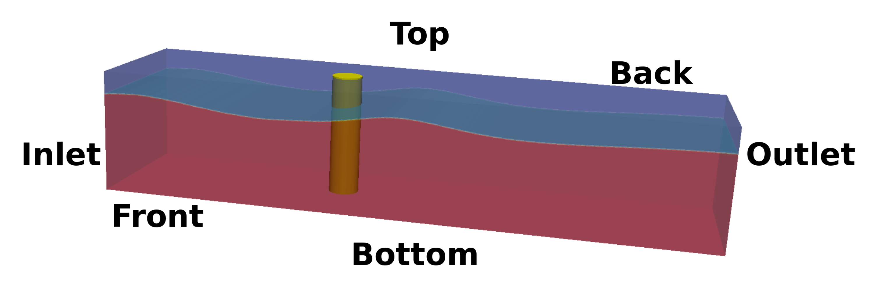
The computational domain is shown in Figure 1, which is 8 m long and 0.4 m wide, the height is 0.8 m. A circular cylinder with a diameter of 0.025 m is fixed at the centerline and the distance between the cylinder and wave generation boundary is 1 m. The wave period, wave height, wave length, initial still water depth, and cylinder diameter in this study are listed in Table 1, which are chosen to be close to parameters for corresponding laboratory experiments [1]. The quantities in Table 1 are preset in model configuration except for the wave length, which is a derived quantity measured from model results. The wave length derived with linear dispersion relation is 3.59 m, this minor difference is induced by the assumptions adopted in the theoretical formulation. The wave generation and absorption methods developed by Higuera et al. [28,29] and Higuera [30] are adopted in this study as no relaxation zone is required, which further reduces the amount of computational resource. The SST two-equation closure model is adopted for turbulence parameterization in this study. A long-standing problem with the VOF method on modeling surface wave dynamics is the severely over-estimated turbulence level along with the phase interface, which dissipates the wave energy significantly and the wave shape could not be maintained. In this study, the modification strategy proposed by Larsen and Fuhrman [31] is utilized to solve this problem.
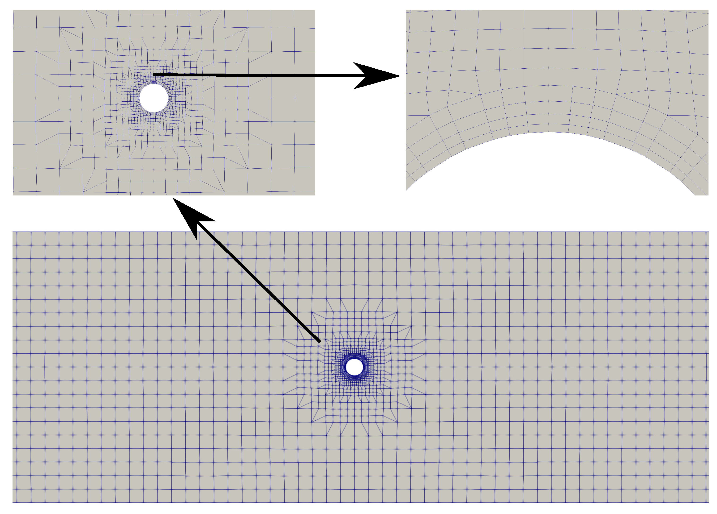
The computational grid topology for a horizontal section is shown in Figure 2, the background mesh with a side length equal to 0.02 m is used across the domain, and the mesh is gradually refined towards the cylinder. A smooth boundary layer with 60 cells adjacent to the cylinder surface is utilized to calculate the forces and moments for each layer on the cylinder. This plane grid structure is extruded 0.8 m along the z axis with 160 homogeneous layers to generate the 3D mesh, the grid resolution along the z direction is 0.005 m, which is fine enough to capture free surface variations. The boundary conditions for the variables in the numerical models are listed in Table 2.
As shown in Section 2, the velocity and acceleration at cylinder location were needed in the Morison equation. These data were not available from laboratory experiments [1], and were derived based on linear wave theory. In order to evaluate the influence of employing this assumption on the determined coefficients, one more numerical simulation is configured to derive velocity and acceleration at cylinder location, the cylinder is removed from the background mesh and no grid refinement is required, the computational domain is divided into cuboid grids with dimensions of 0.02 m × 0.02 m × 0.005 m. The numerical results of velocities and moments are saved every 0.01 s, while other physical quantities are output every 0.05 s to save the storage resources.
4. Result Analysis
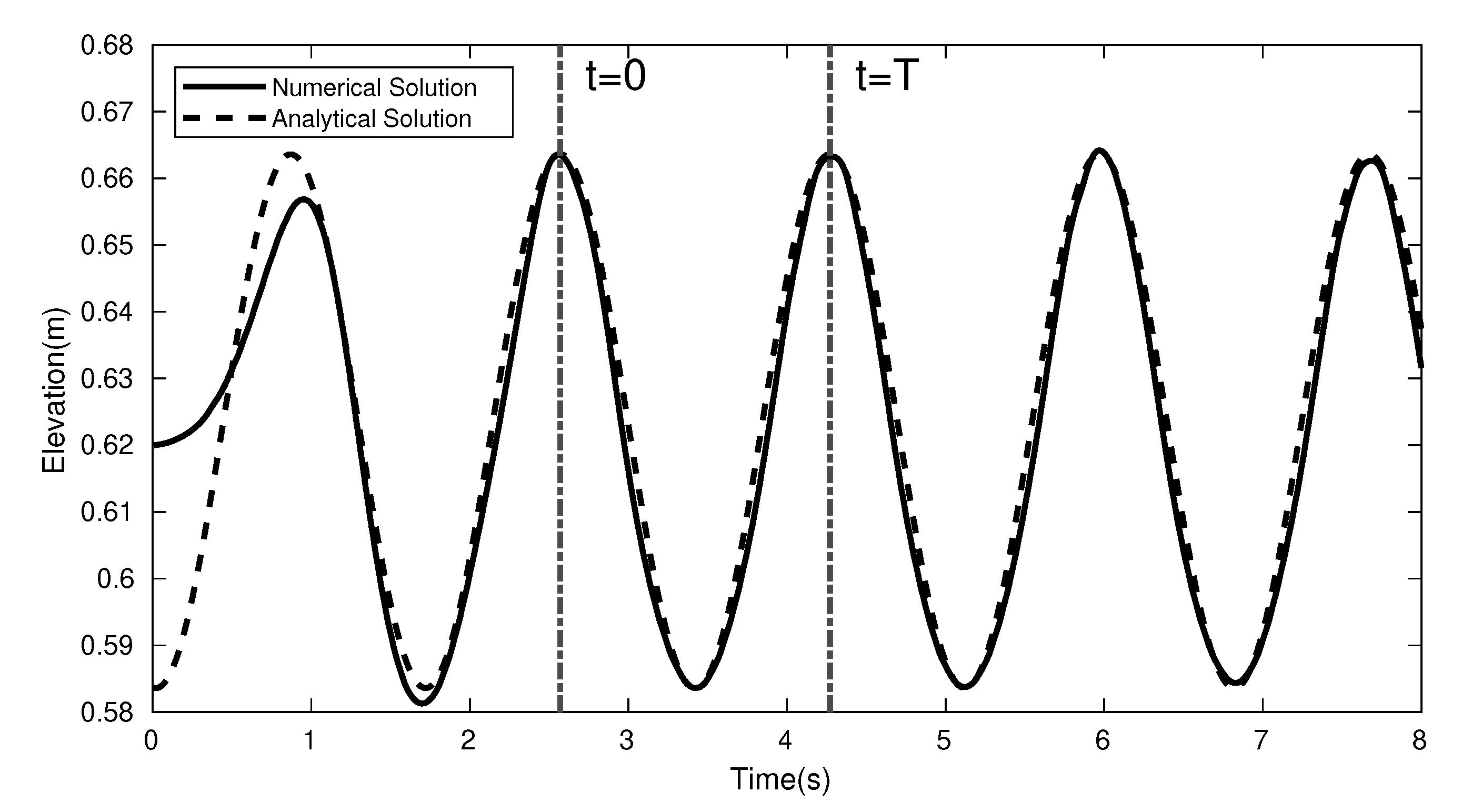
The numerical results are analyzed in this section. The temporal evolution of surface elevations at cylinder location are shown in Figure 3. The analytical solution based on linear wave theory is also plotted for comparison. The analytical solution is translated in time to be in phase with the numerical solution. It can be seen that after the startup duration of about 1 s, the temporal evolution of surface elevations at cylinder location fit the analytical solution reasonably well, which confirms the assumption of the linear wave for this configuration. The two vertical lines mark time steps 2.57 s and 4.27 s, which are designated as and respectively. The wave phases for these two time steps are assigned as and for later discussion, the minus sign is introduced as the wave phase decreases with increasing time for fixed location . The velocity and moment data within this specific period are further analyzed in this section.
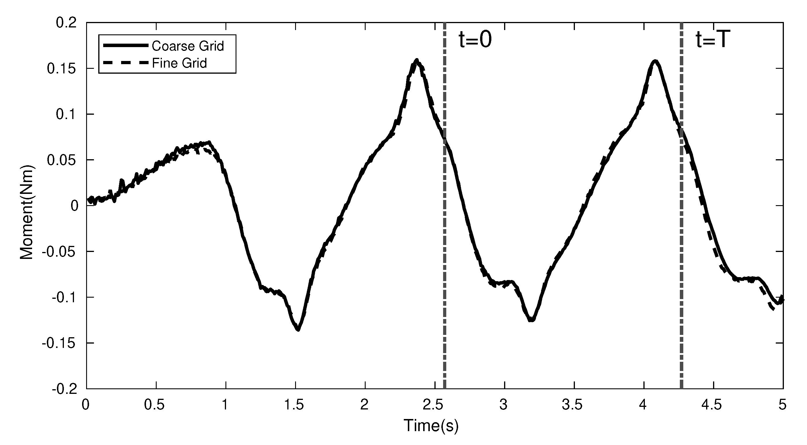
The moments exerted by surface waves on the cylinder are calculated directly with a numerical model and shown in Figure 4. The forces and moments on a rigid structure by fluid motion are known to be very sensitive to the thickness of mesh adjacent to the structure surface. A mesh sensitivity study is performed to check the validity of chosen mesh. Two meshes with similar topology are used, the difference lies in that the thickness of grids adjacent to the cylinder for one mesh is half of that for another mesh, the boundary layer thicknesses close to the cylinder for these two cases are 0.25 mm and 0.5 mm, respectively, these two meshes are referred to as fine mesh and coarse mesh respectively. From Figure 4 it can be seen that the temporal evolution of moments are independent of the meshes chosen and the numerical results can be used for further analysis.
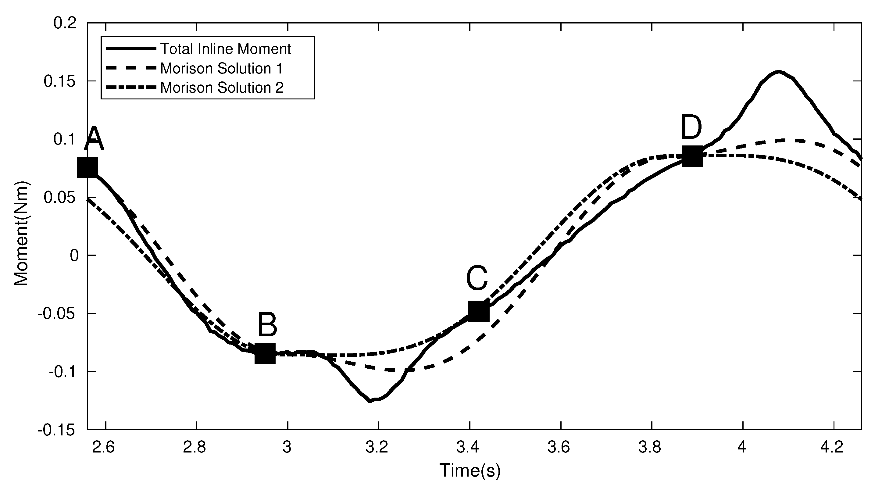
The coefficients and are determined from numerical results with the method proposed by Morison et al. [1] as mentioned in Section 2. The moment values at four specific phases within one period are selected, which corresponds to wave phases , these positions are marked as points A, B, C, and D in Figure 5 respectively. The empirical coefficients are derived with Equations (8) and (9), the values are listed in Table 3. The missing values in the table for the empirical coefficients are introduced as the terms with those coefficients are zero at specific positions, e.g., for positions A and C, the terms including inertial coefficient are zero, only the drag coefficient could be derived. These results could be rewritten in the form of average values with uncertainties, and . It can be seen that the phenomenon observed in the original manuscript by Morison et al. [1] is reproduced, namely, the uncertainties for drag coefficient are much larger than those for inertial coefficient. Before exploring the reason for this discrepancy, the temporal evolution of predicted moments with Equation (5), is shown in Figure 5 to estimate the accuracy of the Morison equation. As coefficients and are needed in the Morison equation, two sets of combinations are used to illustrate their influence on the results. The solution 1 is predicted by the Equation (5) with coefficients and determined from positions A and B, respectively, while the solution 2 is based on the same equation and the corresponding coefficients for positions C and D. Since the inertial coefficients derived from positions B and D are very close, the differences between solution 1 and 2 are predominately induced by the distinct values of drag coefficients. From Figure 5 it can be seen that the predictions with drag coefficient determined by moment value at position A fail to fit the moment value at position C and vice versa. Although both solutions could predict the general trend of calculated moments, some gaps between the predictions and true values are evident, and the extreme value for moments is obviously underestimated by the empirical equation, which is also observed in the original manuscript [1]. It is beneficial to analyze whether these discrepancies could be reduced or the influences of assumptions employed on the predictability of the Morison equation, which could further help improve empirical equation.
One key assumption used by Morison et al. [1] is that the waves can be treated as small-amplitude waves and the nonlinearity could be omitted, which could be partially confirmed from the comparison of surface elevations as shown in Figure 3. It should be noted for linear wave theory that the surface elevation is assumed to be negligibly small that its temporal variations can be neglected for other physical quantities; this significantly simplifies the theoretical formulation, without which analytical solution could not be obtained. With this assumption, the upper boundary for theoretical wave parameters, e.g., the orbital velocity, is shifted from free surface to . This can also be discerned in Equation (4), the total moment is derived by integrating the corresponding value for each differential section from bottom to initial still surface, although the free surface oscillates periodically.
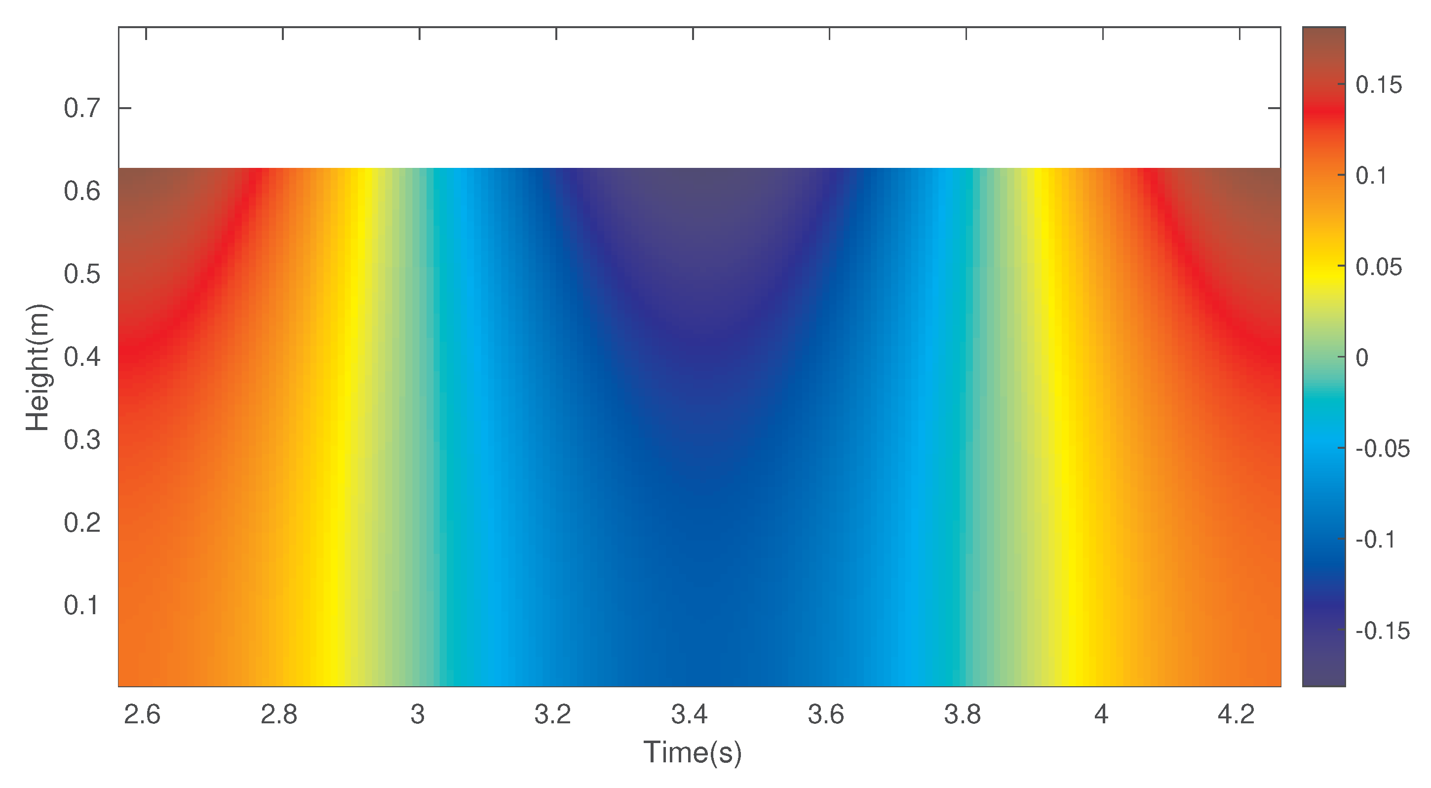
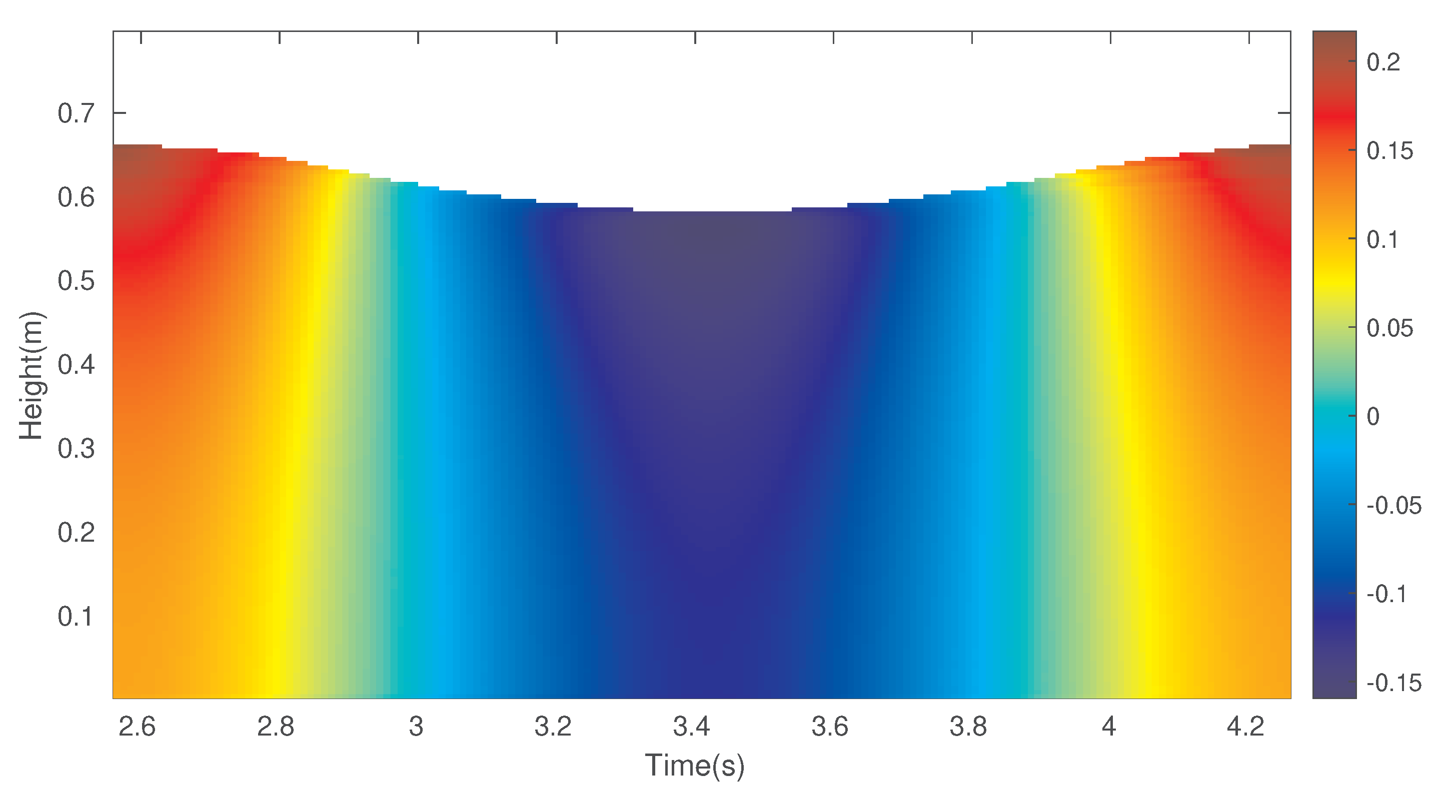
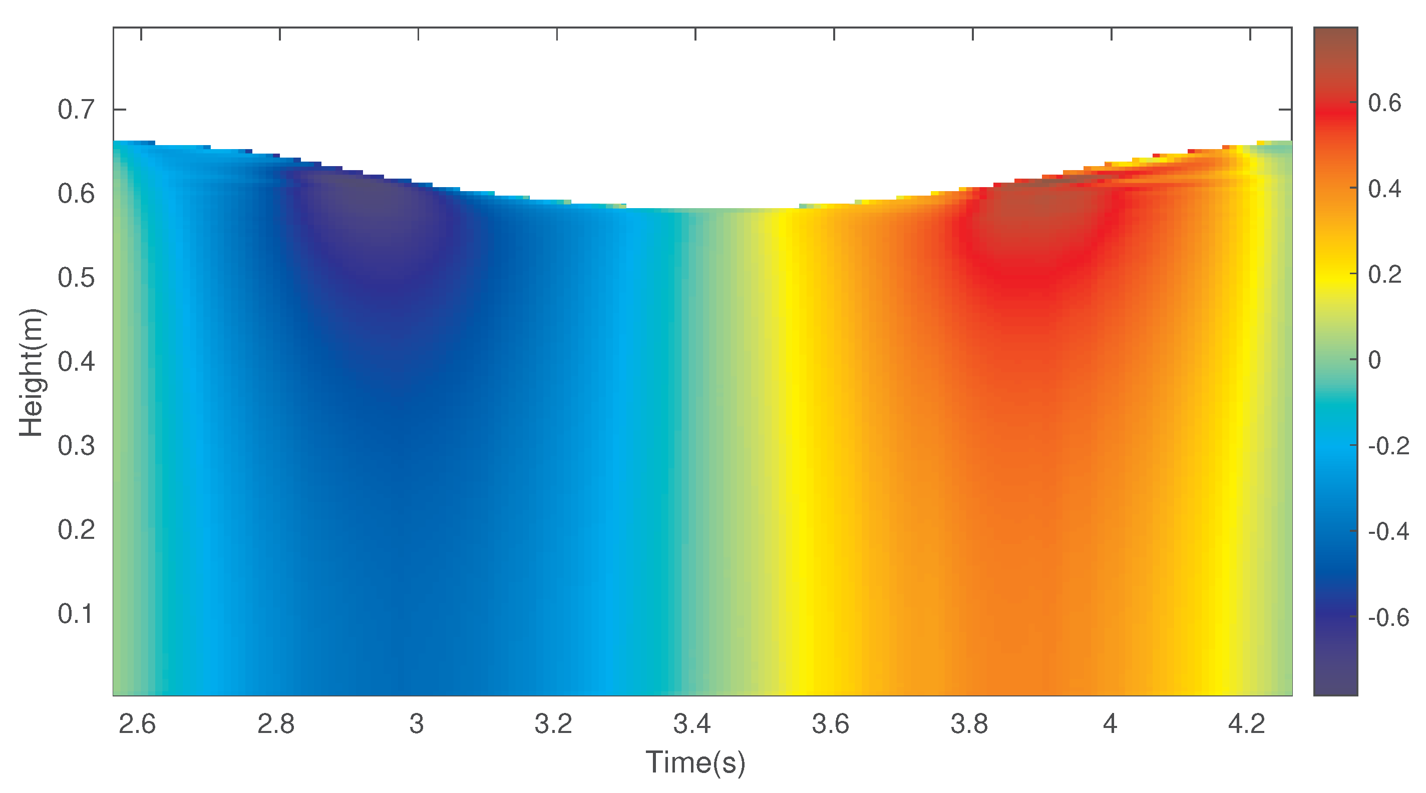
The introduction of linear wave theory is to estimate velocity and acceleration field at cylinder location, which are not available from laboratory experiments, the numerical model can also be used to estimate velocity field and evaluate the accuracy of linear wave theory. An accompanying numerical simulation without cylinder is performed to get the corresponding velocity and acceleration field at cylinder location. The temporal evolution of theoretical and numerical velocity field for one period are shown in Figure 6 and Figure 7. It can be seen that the theoretical formulation (Equation (2)) could depict the general trend of the velocity field reasonably well, except for regions around the free surface. The theoretical expression for velocity field neglects free surface oscillations, which could potentially introduce errors at wave crest and trough, where the drag coefficient is determined.
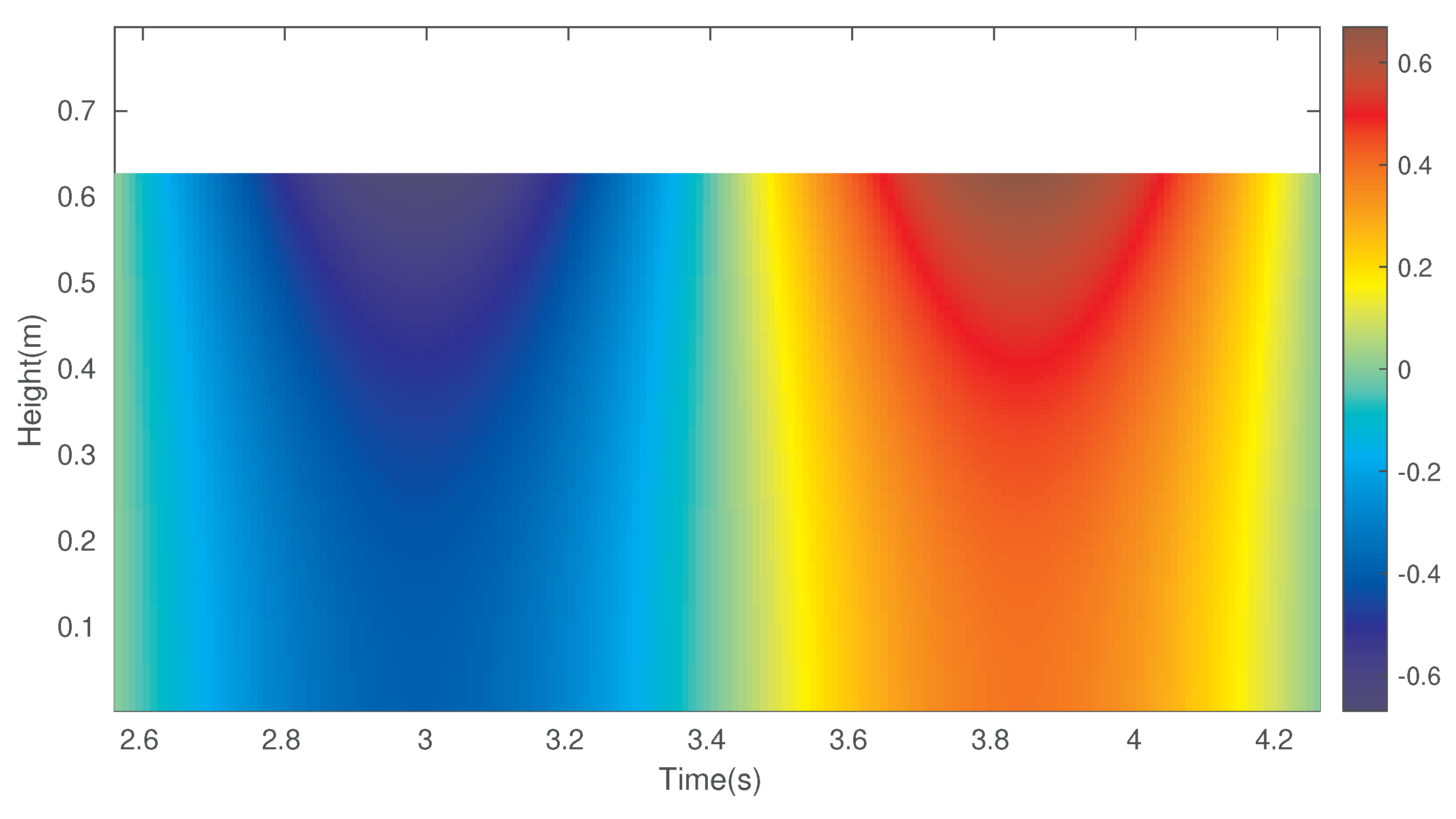
The temporal evolution of theoretical and numerical acceleration fields for one period are shown in Figure 8 and Figure 9. The key differences for these two fields also mostly lie around free surface regions. The acceleration data at phases and are used to derive inertial coefficient , as the actual surface elevations at these two moments are the same as initial still water, the uncertainties for inertial coefficients are relatively smaller. This partially explains why the uncertainties in drag coefficient are larger than those in inertial coefficients with theoretical velocity and acceleration field.
From the above analysis, it can be seen that the theoretical formulations of velocity and acceleration neglect the influence of surface elevations, which could introduce larger uncertainties in the empirical coefficients and predictability of the Morison equation. The numerical solution for velocity field at cylinder location takes this into account and could be used as an alternative for the coefficients determination. The moments for these four-wave phases can be expressed as,
The oscillations of free surface are taken into account in the determination of drag coefficient . The integration on the right hand side of these equations could be approximately expressed as algebraic summation of the corresponding discretized variables, e.g.,
where k is the grid index in the vertical direction, n is the time index, is the time step, which is 0.01 s for the velocity, is the grid space in the vertical direction, which is equal to 0.005 m. The summation index k starts from the bottom cell to the top cell that is cut by the free surface. After the coefficients and are fixed, the temporal evolution of moments could be predicted as,
The coefficients and determined with the numerically derived velocity and acceleration field are shown in Table 4, from which it can be seen that the uncertainties in drag coefficient are significantly reduced, , although they are still larger than those for inertial coefficient . The linear wave theory is assumed in the coefficients determination method proposed by Morison et al. [1], the applicability of this method for other wave scenarios, e.g., nonlinear waves or irregular waves, is thus very limited. The least squares method (LS) is one widely used alternative for empirical coefficients determination [32], which is also tested here for reference. All the data are taken into account with the least-squares method and the minimum mean squared error between model predictions and measurements is used as a metric to fix the coefficients. From Table 4 it can be seen that larger drag and inertial coefficients are derived with the LS method. Other coefficient determination methods, such as the Fourier average, are adopted by Sarpkaya [15], which can only be used for two-dimensional oscillating flows, are not discussed in this study.
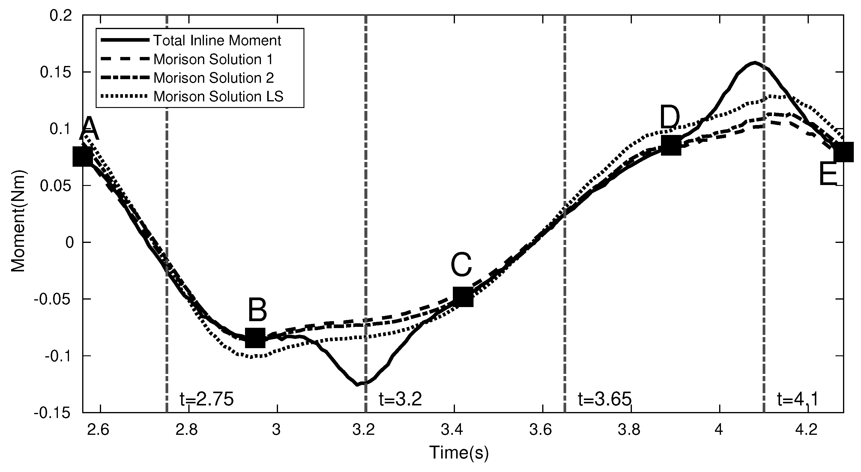
The temporal evolution of moments predicted by Equation (15) with three different combinations of empirical coefficients and the directly calculated moments are compared in Figure 10. The drag coefficient determined by position A and the inertial coefficient determined by position B are employed by solution 1, the corresponding coefficients for positions C and D are used by solution 2, while the coefficients determined by the least-squares method are utilized by solution LS. It can be seen that solutions 1 and 2 are very close to each other, more specifically, solution 1 could fit the moments at positions C and D reasonably well; this is also true for solution 2 at positions A and B, which exhibits superior performance than those shown with the theoretical formulation in Figure 5. However, there exhibit obvious distinctions between these two solutions and calculated moments for different wave phases. These two solutions could fit the calculated moments quite well for some phase ranges, e.g., ranges A–B and C–D, while significant discrepancies exist for other phase ranges, e.g., ranges B–C and D–E. The solution LS is anticipated to perform better as the coefficients are determined by minimizing the differences between predictions and true values. The solution LS with larger drag and inertial coefficients could predict higher maximum moment values, however, there still exist significant discrepancies between predictions and true moments. Furthermore, the solution LS fails to fit most of the selected positions, e.g., positions A, B and D.
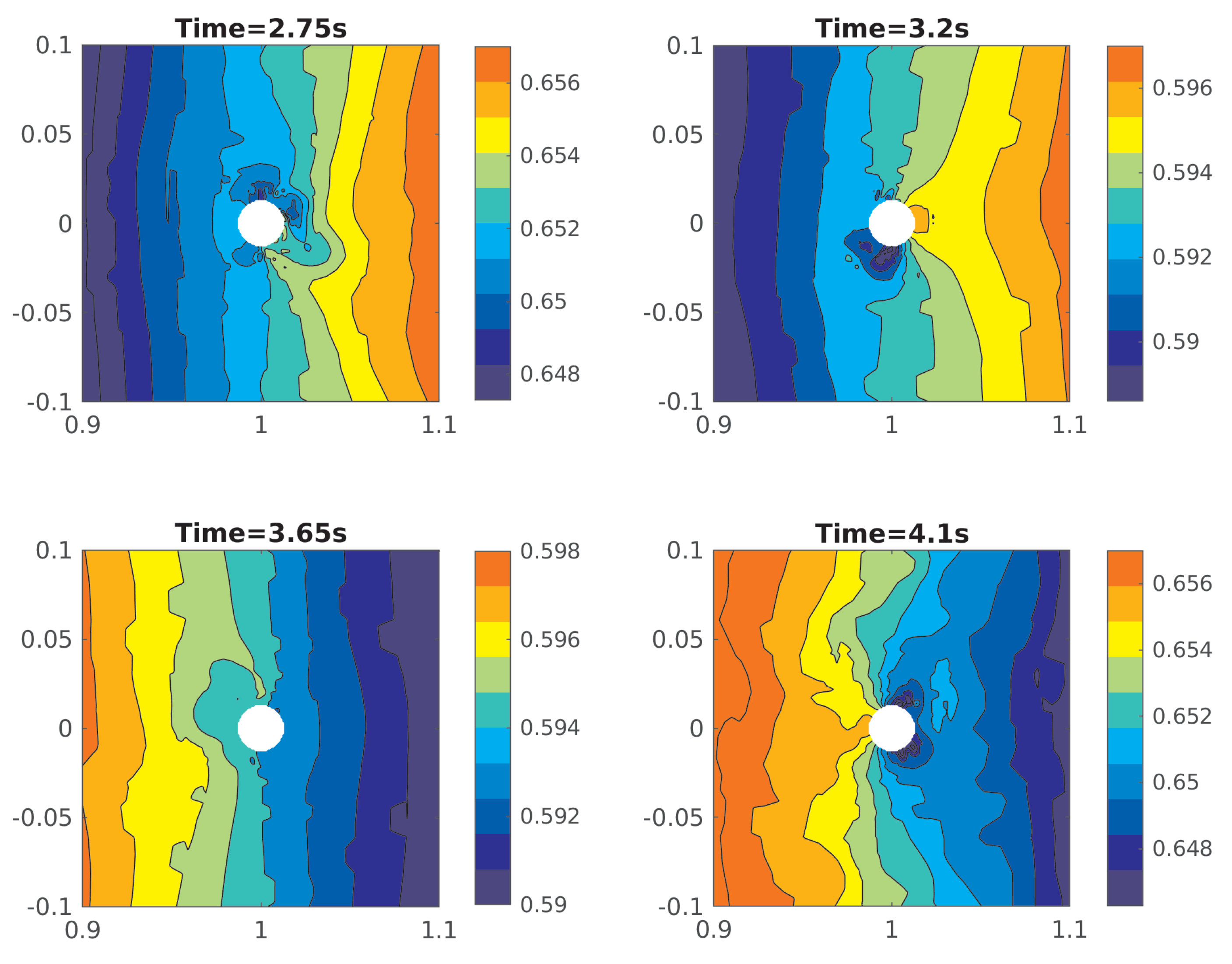
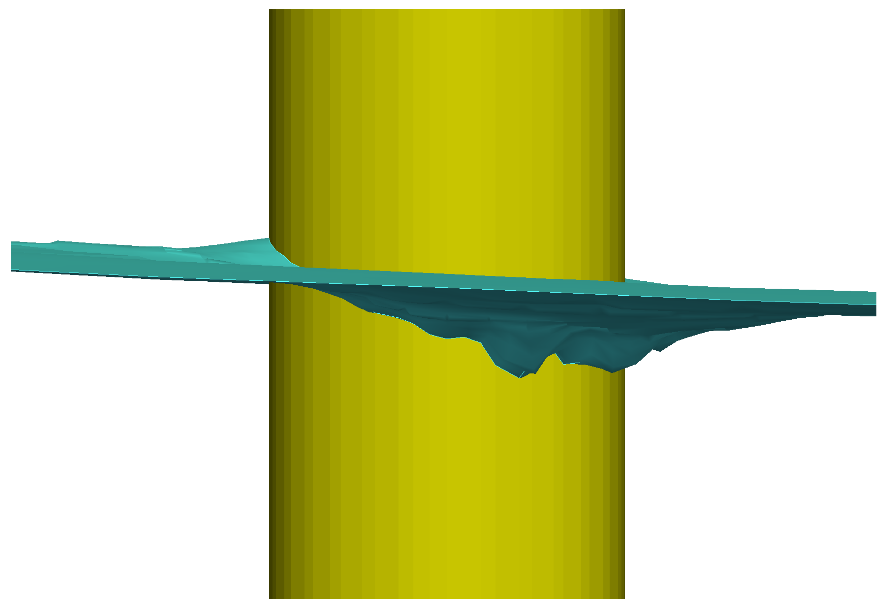
The numerical data at four times ( s, 3.2 s, 3.65 s, and 4.1 s) are chosen to investigate the mechanism for this phenomena further. The surface elevations around the cylinder for these four times are shown in Figure 11. The surface elevations are derived by calculating vertical coordinates of isosurface with linear interpolation and these elevations are then mapped to one regular grid with bilinear interpolation. It can be seen that for the times 2.75 s and 3.65 s, the isolines of the free surface around the cylinder location are approximately parallel to those away from it, although some noises exist around the cylinder, which could be induced by weak wave-cylinder interactions. This confirms the assumption that the surface wave is not disturbed by the cylinder, and the predictions with the Morison equation could fit the calculated moments quite well. The surface elevations for the other two times 3.2 s and 4.1 s, however, exhibit distinct characteristics, the isolines of the free surface around the cylinder are out of shape, resulting in wave run-up on one side of the cylinder. The wave run-up phenomenon is induced by the existence of a cylinder, which could be discerned as an elevated water surface as the local flow is blocked by obstacles as shown in Figure 12.
These wave run-up processes produce additional local forces and moments on the cylinder, which could explain the discrepancies between predictions by the Morison equation and directly calculated values, as the wave run-up process is not taken into account in the Morison equation. The physical mechanism for wave run-up could be readily explained. For the time ranges B–C and D–E, the wave induced velocity and acceleration field at cylinder location are in the same direction, in other words, the water particles are moving towards cylinder with increasing velocity, the wave-cylinder interaction, or blocking effect by cylinder produces an additional amount of elevated water adjacent to the cylinder. For the time ranges A–B and C–D, the velocity and acceleration at cylinder location are in opposite directions, the water particles move towards cylinder with decreasing velocity, the wave run-up is not generated or negligibly small for this scenario. As a short summary, the local wave run-up process results in an additional loading on the cylinder, the scale of which is approximately the diameter of the cylinder, as can be discerned in Figure 11.
Morison et al. [1] proposed that if the diameter of the pile is much less than the wave length, , the incident wave field could be treated as not being disturbed and the existence of the cylinder can be neglected. The ratio of cylinder diameter to wave length for the present configuration is about 0.007, which is one order of magnitude smaller than the criterion assumed by Morison et al. [1]. The numerical results show that for such a small cylinder, the influence of the cylinder on wave field is quite small, except for a region adjacent to the cylinder with a scale of cylinder diameter. Although the length of this region is significantly smaller than the wave length, the influence by local wave run-up could not be neglected as the integrated wave loads highly depend on the flow field adjacent to the cylinder.
This is not the first manuscript that notices the influences of local wave surface distortions on the forces and moments exerted on the cylinder. Several previous studies have noticed these phenomena, which are expected to cause high-frequency loads on the cylinder [19,20,23,25], although different terms are used to describe this, e.g., ‘mound’ [20] or ‘upwelling’ [25]. Previously this phenomenon is primarily studied for nonlinear waves, e.g., fifth-order Stokes waves [25] and irregular waves [19,20,23,33,34]. The cylinder diameters in these studies are also much larger than that in this study, e.g., the minimum non-dimensional radius in the experiments by Li et al. [33,34] is 0.32, while the quantity from the present study is 0.023. In this study, it is found that the wave run-up process also exists for linear waves, and the scale of this phenomenon is approximately cylinder diameter, as shown in Figure 11, which is the same as those observed for nonlinear waves [19,23,25]. The frequencies of local wave run-up, however, are different among these scenarios. For nonlinear waves, the local wave run-up is only prominent at one side of the cylinder and occurs once per period, which can be explained as the incident velocity at the free surface is quite different if there comes an incident wave crest or wave trough [25]. For the linear wave scenario, the differences between incident velocity accompanied with wave crest and trough are marginal, the wave run-up could exist at both sides of the cylinder, and their magnitudes are comparable, two wave run-up processes can be observed within one period.
MacCamy and Fuchs [35] analyzed the wave forces on the pile with a diffraction theory, the assumption adopted therein was very close to the configurations of this study, e.g., the small ratio of wave height to its length, the diameter of the cylinder was small compared to the wave length. Large deviations exist between the theoretical predictions and experimental results. The reason for this rather large discrepancy was discussed and attributed to the inviscid fluid assumption, the fluid motion was symmetrical around the cylinder and no separation occurred, resulting in zero drag contribution.
It can be seen from Table 4 there exist distinct discrepancies between the empirical coefficients derived with different methods for one set of measurements, which are also confirmed for irregular waves [32]. For the two methods used in the present study, e.g., the method proposed by Morison et al. [1] and the widely used least-squares method, it is beneficial to discuss the pros and cons of these two methods. The least squares method is the best choice if mean squared error is used as the metric, however, as certain physical process, e.g., wave run-up, is not taken into account in Morison formula, the coefficients are unavoidably influenced by the unresolved process. The coefficients derived with this method perform better for the available data, but their generalization for unseen data is not reliable. For the alternative method proposed by Morison et al. [1], the data at selected times are used to fix drag and inertial coefficients when the wave run-up effects are negligibly small. The coefficients derived with this method behave better than those inferred with least-squares counterpart for the temporal ranges when wave run-up is relatively small and fail to fit the true values when wave run-up dominates, as shown in Figure 10.
Morison equation has now widely accepted in the industry to estimate wave loads on cylinder structure, although the coefficients proposed in the original manuscript are seldom used. Sarpkaya [15] proposed that the inertial and drag coefficients were functions of Reynolds and Keulegan–Carpenter numbers, however, it should be noted that their coefficients were based on measurements in a U-shaped oscillating-flow tunnel, wherein surface elevations were suppressed. In industry standard, e.g., American Petroleum Institute (API) Recommended Practice, constant values for the coefficients are suggested for realistic scenarios, and , which are close to the results by Sarpkaya [15] for high Reynolds numbers. The wave run-up processes are therefore not taken into account with these coefficients, which could potentially underestimate realistic forces and moments.
Recently Zan and Lin [12] examined the applicability of the Morison equation on the force estimation by internal solitary waves on cylindrical structure, and found that the total acceleration should be used as the nonlinearity could not be neglected. The significance of nonlinearity is also evaluated for this study, which is indeed negligibly small and the result is not shown for brevity.
Lastly, it should be noted that moments were measured in Morison et al. [1], in later studies, the forces on cylinder could also be readily measured. The theoretical formula for integrated forces is much simpler than that for integrated moments. Similar conclusions could be drawn if the forces are used to determine the empirical coefficients and are not shown here for brevity. The moments are used in this study to make it consistent with the study by Morison et al. [1].
5. Conclusions
In this manuscript, the empirical equation proposed by Morison et al. [1] is revisited and numerical simulation is utilized to reproduce the corresponding laboratory experiments with similar configurations. The primary purpose is to address some issues observed in the original paper, e.g., larger uncertainties for drag coefficient and underestimated maximum moments.
The larger uncertainties for drag coefficient are successfully reproduced with model results and coefficients determination method proposed by Morison et al. [1], in which linear wave theory is adopted to derive the velocity and acceleration field in Morison equation. The surface elevations are neglected in the velocity expression for linear wave theory, which could potentially introduce larger uncertainties in the drag coefficient. The numerical model is utilized to reproduce the velocity field at cylinder location, which are more realistic as the temporal variations of surface elevation are taken into account. The uncertainties of drag coefficients derived with model-based velocity and acceleration field are significantly reduced, which confirms the influences of linear wave theory on the determined empirical coefficients.
The numerical model could also reproduce the phenomenon that maximum moments are underestimated by the Morison equation, the analysis reveals that the additional loads are caused by local wave run-up. The run-up is not restricted to the immediate vicinity of the cylinder, but extends about the length of cylinder diameter, which is the same as those for nonlinear wave scenarios. There are two prominent and comparable wave run-up processes around the cylinder within one period for linear wave case, while there exists only one distinct wave run-up process for nonlinear waves. The Morison equation should be used with caution as it does not consider the influence of the wave run-up process, which could potentially underestimate the loads by surface waves on the cylindrical structure. The present study reveals that although most recent studies are focusing on the mechanisms of high-frequency loads introduced by nonlinear waves on cylinders, there are still some issues to be addressed for the linear waves. Further studies are required to analyze the dependence of additional loads induced by the wave run-up process on the wave and cylinder parameters, the results of which could strengthen the reliability of the Morison equation and provide dependable predictions for the industry during designing stage.
Author Contributions
Conceptualization, Z.L. and Y.G.; methodology, Z.L.; software, Z.L.; formal analysis, X.Z.; writing—original draft preparation, X.Z.; writing—review and editing, X.Z., Y.G. and Z.L.; funding acquisition, Z.L. and X.Z. All authors have read and agreed to the published version of the manuscript.
Funding
ZXX is supported by National Natural Science Foundation of China (No. 32102795), LZH is supported by Shandong Provincial Natural Science Foundation, China (ZR2021MD078) and the Open Fund of State Key Laboratory of Coastal and Offshore Engineering, Dalian University of Technology with grant No. LP2003.
Institutional Review Board Statement
Not applicable.
Informed Consent Statement
Not applicable.
Data Availability Statement
Not applicable.
Conflicts of Interest
The authors declare no conflict of interest.
References
- Morison, J.R.; Johnson, J.W.; Schaaf, S.A. The force exerted by surface waves on piles. J. Pet. Technol. 1950, 2, 149–154. [Google Scholar] [CrossRef]
- Wang, J.; Song, J.; Huang, Y.; Fan, C. On the parameterization of drag coefficient over sea surface. Acta Oceanol. Sin. 2013, 32, 68–74. [Google Scholar] [CrossRef]
- Wang, Z.; Duan, C.; Dong, S. Long-term wind and wave energy resource assessment in the South China sea based on 30-year hindcast data. Ocean Eng. 2018, 163, 58–75. [Google Scholar] [CrossRef]
- Li, R.; Wu, K.; Li, J.; Akhter, S.; Dong, X.; Sun, J.; Cao, T. Large-Scale Signals in the South Pacific Wave Fields Related to ENSO. J. Geophys. Res. Ocean. 2021, 126. [Google Scholar] [CrossRef]
- Wang, J.; Li, B.; Gao, Z.; Wang, J. Comparison of ECMWF Significant Wave Height Forecasts in the China Sea with Buoy Data. Weather Forecast. 2019, 34, 1693–1704. [Google Scholar] [CrossRef]
- Wang, Z.; Wu, K.; Xia, C.; Zhang, X. The impact of surface waves on the mixing of the upper ocean. Acta Oceanol. Sin. 2014, 33, 32–39. [Google Scholar] [CrossRef]
- Lin, X.; Wang, S.; Zhu, B. Effect of uniform incoming flow on vehicle’s hydrodynamics under the same relative velocity. Ocean Eng. 2021, 237, 109491. [Google Scholar] [CrossRef]
- Lin, X.; Xiong, L. Hydrodynamic force acted on a solid translating in nonuniform stream. Ocean Eng. 2021, 241, 110033. [Google Scholar] [CrossRef]
- Cai, S.Q.; Long, X.M.; Gan, Z.J. A method to estimate the forces exerted by internal solitons on cylindrical piles. Ocean Eng. 2003, 30, 673–689. [Google Scholar] [CrossRef]
- Cai, S.Q.; Wang, S.G.; Long, X.M. A simple estimation of the force exerted by internal solitons on cylindrical piles. Ocean Eng. 2006, 33, 974–980. [Google Scholar] [CrossRef]
- Si, Z.; Zhang, Y.; Fan, Z. A numerical simulation of shear forces and torques exerted by large-amplitude internal solitary waves on a rigid pile in South China Sea. Appl. Ocean Res. 2012, 37, 127–132. [Google Scholar] [CrossRef]
- Zan, X.X.; Lin, Z.H. On the applicability of Morison equation to force estimation induced by internal solitary wave on circular cylinder. Ocean Eng. 2020, 198, 106966. [Google Scholar] [CrossRef]
- Lin, Z.; Zan, X. Numerical study on load characteristics by internal solitary wave on cylinder sections at different depth and its parameterization. Ocean Eng. 2021, 219, 108343. [Google Scholar] [CrossRef]
- Zan, X.; Lin, Z.; Gou, Y. Numerical study on the force distribution on cylindrical structure by internal solitary wave and its prediction with Morison equation. Ocean Eng. 2022, 248, 110701. [Google Scholar] [CrossRef]
- Sarpkaya, T. Vortex Shedding and Resistance in Harmonic Flow about Smooth and Rough Circular Cylinders at High Reynolds Numbers; Technical Report; Naval Postgraduate School: Monterey, CA, USA, 1976. [Google Scholar]
- Sarpkaya, T. Force on a circular cylinder in viscous oscillatory flow at low Keulegan—Carpenter numbers. J. Fluid Mech. 1986, 165, 61. [Google Scholar] [CrossRef]
- Stokes, G. On the effect of the internal friction of fluids on the motion of pendulums. Trans. Camb. Philos. Soc. 1851, 9, 8–106. [Google Scholar]
- Wang, C.Y. On high-frequency oscillatory viscous flows. J. Fluid Mech. 1968, 32, 55–68. [Google Scholar] [CrossRef]
- Riise, B.H.; Grue, J.; Jensen, A.; Johannessen, T.B. High frequency resonant response of a monopile in irregular deep water waves. J. Fluid Mech. 2018, 853, 564–586. [Google Scholar] [CrossRef]
- Chaplin, J.R.; Rainey, R.C.T.; Yemm, R.W. Ringing of a vertical cylinder in waves. J. Fluid Mech. 1997, 350, 119–147. [Google Scholar] [CrossRef]
- Grue, J.; Huseby, M. Higher-harmonic wave forces and ringing of vertical cylinders. Appl. Ocean Res. 2002, 24, 203–214. [Google Scholar] [CrossRef]
- Paulsen, B.T.; Bredmose, H.; Bingham, H.B.; Jacobsen, N.G. Forcing of a bottom-mounted circular cylinder by steep regular water waves at finite depth. J. Fluid Mech. 2014, 755, 1–34. [Google Scholar] [CrossRef]
- Riise, B.H.; Grue, J.; Jensen, A.; Johannessen, T.B. A note on the secondary load cycle for a monopile in irregular deep water waves. J. Fluid Mech. 2018, 849, R1. [Google Scholar] [CrossRef]
- Fan, X.; Zhang, J.; Liu, H. Numerical analysis on the secondary load cycle on a vertical cylinder in steep regular waves. Ocean Eng. 2018, 168, 133–139. [Google Scholar] [CrossRef]
- Kristiansen, T.; Faltinsen, O.M. Higher harmonic wave loads on a vertical cylinder in finite water depth. J. Fluid Mech. 2017, 833, 773–805. [Google Scholar] [CrossRef] [Green Version]
- Hirt, C.; Nichols, B. Volume of fluid (VOF) method for the dynamics of free boundaries. J. Comput. Phys. 1981, 39, 201–225. [Google Scholar] [CrossRef]
- Chen, L.; Zang, J.; Hillis, A.; Morgan, G.; Plummer, A. Numerical investigation of wave–structure interaction using OpenFOAM. Ocean Eng. 2014, 88, 91–109. [Google Scholar] [CrossRef] [Green Version]
- Higuera, P.; Lara, J.L.; Losada, I.J. Realistic wave generation and active wave absorption for Navier–Stokes models. Coast. Eng. 2013, 71, 102–118. [Google Scholar] [CrossRef]
- Higuera, P.; Lara, J.L.; Losada, I.J. Simulating coastal engineering processes with OpenFOAM®. Coast. Eng. 2013, 71, 119–134. [Google Scholar] [CrossRef]
- Higuera, P. Enhancing active wave absorption in RANS models. Appl. Ocean Res. 2020, 94, 102000. [Google Scholar] [CrossRef]
- Larsen, B.E.; Fuhrman, D.R. On the over-production of turbulence beneath surface waves in Reynolds-averaged Navier–Stokes models. J. Fluid Mech. 2018, 853, 419–460. [Google Scholar] [CrossRef] [Green Version]
- Raed, K.; Guedes Soares, C. Variability effect of the drag and inertia coefficients on the Morison wave force acting on a fixed vertical cylinder in irregular waves. Ocean Eng. 2018, 159, 66–75. [Google Scholar] [CrossRef]
- Li, J.; Wang, Z.; Liu, S. Experimental study of interactions between multi-directional focused wave and vertical circular cylinder, Part I: Wave run-up. Coast. Eng. 2012, 64, 151–160. [Google Scholar] [CrossRef]
- Li, J.; Wang, Z.; Liu, S. Experimental study of interactions between multi-directional focused wave and vertical circular cylinder, part II: Wave force. Coast. Eng. 2014, 83, 233–242. [Google Scholar] [CrossRef]
- MacCamy, R.C.; Fuchs, R.A. Wave Forces on Piles: A Diffraction Theory; Technical Report; The Institute of Engineering Research, University of California: Los Angeles, CA, USA, 1954. [Google Scholar]
Figure 1.
The computational domain and the boundaries (Perspective View).

Figure 2.
The computational grid topology around cylinder.

Figure 3.
The comparison of surface elevations from numerical model and linear wave theory.

Figure 4.
Temporal evolution of the moments on cylinder.

Figure 5.
Comparison of moments calculated from model and Morison equation for .

Figure 6.
The temporal evolution of horizontal velocity at cylinder location (Analytical solution).

Figure 7.
The temporal evolution of horizontal velocity at cylinder location (Numerical solution).

Figure 8.
The temporal evolution of horizontal acceleration at cylinder location (Analytical solution).
Figure 8.
The temporal evolution of horizontal acceleration at cylinder location (Analytical solution).

Figure 9.
The temporal evolution of horizontal acceleration at cylinder location (Numerical solution).
Figure 9.
The temporal evolution of horizontal acceleration at cylinder location (Numerical solution).

Figure 10.
The comparison of moments estimated by different coefficients determination method.

Figure 11.
The surface elevations around the cylinder at different times.

Figure 12.
The surface elevations around cylinder at 4.1 s.


Table 1.
The wave period T, wave height H, wave length L, initial still water depth h, cylinder diameter D in Morison et al. [1] and this study.
Table 1.
The wave period T, wave height H, wave length L, initial still water depth h, cylinder diameter D in Morison et al. [1] and this study.
| Parameter | T | H | L | h | D |
|---|---|---|---|---|---|
| Morison et al. [1] | 1.68 s | 0.0744 m | 3.734 m | 0.6187 m | 0.0253 m |
| Numerical Setting | 1.7 s | 0.08 m | 3.43 m | 0.62 m | 0.025 m |
Table 2.
The boundary conditions of the key variables in the computation.
| Variable | U | ||
|---|---|---|---|
| Inlet | waveAlpha | fixedFluxPressure | waveVelocity |
| Outlet | zeroGradient | fixedFluxPressure | waveAbsorptionVelocity |
| Front/Back | zeroGradient | fixedFluxPressure | noSlip |
| Top | inletOutlet | totalPressure | pressureInletOutletVelocity |
| Bottom | zeroGradient | fixedFluxPressure | noSlip |
| Cylinder | zeroGradient | fixedFluxPressure | noSlip |
Table 3.
The empirical coefficients and derived with velocity field based on linear wave theory.
| Position | A | B | C | D |
|---|---|---|---|---|
| Phase | 0 | |||
| 1.506 | - | 0.961 | - | |
| - | 1.685 | - | 1.705 |
Table 4.
The empirical coefficients and derived with velocity field based on numerical simulation.
| Position | A | B | C | D | LS |
|---|---|---|---|---|---|
| Phase | 0 | - | |||
| 1.086 | - | 1.215 | - | 1.352 | |
| - | 1.618 | - | 1.664 | 1.935 |
Publisher’s Note: MDPI stays neutral with regard to jurisdictional claims in published maps and institutional affiliations. |
© 2022 by the authors. Licensee MDPI, Basel, Switzerland. This article is an open access article distributed under the terms and conditions of the Creative Commons Attribution (CC BY) license (https://creativecommons.org/licenses/by/4.0/).
Share and Cite
MDPI and ACS Style
Zan, X.; Lin, Z.; Gou, Y. The Force Exerted by Surface Wave on Cylinder and Its Parameterization: Morison Equation Revisited. J. Mar. Sci. Eng. 2022, 10, 702. https://0-doi-org.brum.beds.ac.uk/10.3390/jmse10050702
AMA Style
Zan X, Lin Z, Gou Y. The Force Exerted by Surface Wave on Cylinder and Its Parameterization: Morison Equation Revisited. Journal of Marine Science and Engineering. 2022; 10(5):702. https://0-doi-org.brum.beds.ac.uk/10.3390/jmse10050702
Chicago/Turabian StyleZan, Xiaoxiao, Zhenhua Lin, and Ying Gou. 2022. "The Force Exerted by Surface Wave on Cylinder and Its Parameterization: Morison Equation Revisited" Journal of Marine Science and Engineering 10, no. 5: 702. https://0-doi-org.brum.beds.ac.uk/10.3390/jmse10050702
Note that from the first issue of 2016, this journal uses article numbers instead of page numbers. See further details here.