Article

Energetic and Ecological Effects of the Slow Steaming Application and Gasification of Container Ships

1
The Maritime Department, University of Zadar, Ulica Mihovila Pavlinovića 1, 23000 Zadar, Croatia
2
Faculty of Mechanical Engineering and Naval Architecture, University of Zagreb, Ivana Lučića 5, 10000 Zagreb, Croatia
*
Author to whom correspondence should be addressed.
J. Mar. Sci. Eng. 2022, 10(5), 703; https://0-doi-org.brum.beds.ac.uk/10.3390/jmse10050703
Submission received: 8 April 2022 / Revised: 9 May 2022 / Accepted: 18 May 2022 / Published: 20 May 2022
(This article belongs to the Special Issue Marine Navigation and Safety at Sea)

Abstract

:
One of the short-term operational measures for fuel savings and reducing CO2 emissions from ships at sea is sailing at reduced speed, i.e., slow steaming, while the gasification of the ship represents an important mid-term technical measure. In this study, the energetic and ecological benefits of slow steaming and gasification are studied for a container ship sailing between Shanghai and Hamburg. Resistance and propulsion characteristics in calm water are calculated using computational fluid dynamics based on the viscous flow theory for a full-scale ship, while the added resistance in waves is calculated by applying potential flow theory. The propeller operating point is determined for the design and slow steaming speeds at sea states with the highest probability of occurrence through the investigated sailing route. Thereafter, the fuel consumption and CO2 emissions are calculated for a selected dual fuel engine in fuel oil- and gas-supplying modes complying with IMO Tier II and Tier III requirements. The results demonstrate a significant reduction in fuel consumption and CO2 emissions for various slow steaming speeds compared to the design speed at different sea states, and for the gasification of a container ship. For realistic weather conditions through the investigated route, the potential reduction in CO2 emissions per year could be up to 11.66 kt/year for fuel oil mode and 8.53 kt/year for gas-operating mode. CO2 emission reduction per year due to gasification under realistic weather conditions could be up to 22 kt/year.

1. Introduction

Global climate change as a significant variation in average weather conditions is currently one of the most important issues. The main cause of climate change is the emission of greenhouse gases (GHG), mostly carbon dioxide (CO2) and methane (CH4). Amongst others, climate change is manifested through an increase in the global average temperature, which then leads to an increased rate of evaporation causing intense storms and weather extremes [1]. For that reason, the ratification of the Paris agreement in 2015 has imposed a limit for global average temperature well below 2 °C, and preferably limited to an increase of 1.5 °C compared to preindustrial levels [2]. However, to achieve this aim GHG emissions should be reduced immediately and reach net zero by the middle of the 21st century. It should be noted that 16.2% of global GHG emissions are caused by the transport sector [3] and the reduction in GHG emissions within the transport sector is crucial. Considering that more than 80% of the international trade in goods is carried by sea, maritime transport is the backbone of international trade and the global economy [4]. Consequently, maritime transport is faced with increasing pressure to decarbonize and operate more sustainably. The interest from the stakeholders of the shipping sector concerning deep decarbonization is increasing. However, decarbonization requires financial incentives and policies at international and regional levels [5]. Although during the last decade the world fleet has become more energy efficient, total GHG emissions are continuously growing. A large portion in GHG emissions in the maritime sector comes from container ships, particularly older and less energy efficient ones. Bearing in mind that the container shipping industry is one of the main transport industries in the maritime sector, the GHG emissions reduction for container ships becomes imperative. It should be noted that most of the world fleet is still powered by carbon-based fuels causing the emission of harmful gases. The fourth International Maritime Organization (IMO) GHG study stated that the share of emissions caused by ships in global anthropogenic emissions has increased from 2.76% in 2012 to 2.89% in 2018 [6], and emissions are projected to increase further. In June 2021, IMO adopted amendments to Annex VI of the MARPOL Convention [7] to reduce the carbon intensity of ships and include targets for energy efficiency, to additionally reduce GHG emissions from ships. The newly adopted measures will require all ships to calculate their energy efficiency existing ship index (EEXI) following technical means to improve their energy efficiency and to establish their annual operational carbon intensity indicator (CII) and CII rating. Carbon intensity relates GHG emissions to the transport work of ships. In addition to GHG emissions, the maritime transport industry significantly contributes to the non-GHG emissions, i.e., sulfur dioxides and nitrogen oxides, which are very harmful to the environment as well [8]. IMO has established emission control areas (ECAs), as an important measure to reduce and control SOx, NOx, and particulate matter (PM) emissions. With the establishment of ECAs, ship operators must decide whether to comply with ECA regulations, which strategy they should adopt to comply with ECA regulations, and establish the ways to minimize associated costs [9]. The possible solutions are fuel switching, i.e., using fuel with higher sulfur content when sailing outside the ECAs, and fuel with lower sulfur content inside the ECAs, installment of scrubbers, or using clean liquefied natural gas (LNG) as fuel. Although the optimal response strategy to adopt ECA regulations is the ECA evasion strategy when the fuel price ratio is greater than the minimum fuel price ratio (critical threshold), ECA evasion strategy is a decision that the ship will increase its sailing distance outside the ECA to reduce the sailing distance within the ECA. However, an evasion strategy will eventually increase the total emissions of harmful gasses.
Numerous measures have been proposed by IMO from 2011 onward to reduce CO2 emissions from the maritime transport industry. These measures are categorized as short-term, mid-term, and long-term measures. One of the short-term measures is the reduction in operating speed of ships called slow steaming. The introduction of slow steaming leads to a decrease in fuel consumption and consequently CO2 emission [10], and is employed by almost all global shipping companies. Although Maersk Lines introduced slow steaming in container shipping, tankers and bulk carriers have adopted it as well [11]. Although slow steaming is associated with environmental benefits, shipping companies often do not recognize slow steaming as a direct measure to increase environmental performance, but whether their customers will be willing to bear the additional costs [12]. In other words, the introduction of slow steaming can increase the round-trip time by 10–20%, depending on the sailing route and port times [13,14], thus reducing the shipping income. An increase in transport time due to slow steaming could lead to an increase in the required number of ships, and in that way the savings in fuel consumption and CO2 emission could decrease significantly. It should be noted that sailing at a speed lower than the ship design speed changes the operating conditions of the engine that could operate in suboptimal conditions [15]. In inland navigation, slow steaming as an operational measure is less achievable [16] considering that power demands are generally significantly different for upstream and downstream with continuous water level fluctuations.
Another possible short-term measure is the development of technical and operational energy efficiency measures for both new and existing ships. LNG fueled ships seem to be technically the most practical alternative to decrease CO2 emissions in deep-sea shipping since LNG can replace conventional, more-polluting oil-based fuels, and enable almost complete removal of SOx and PM emissions with a substantial reduction in NOx emissions as well [17]. While LNG carriers have used LNG as fuel for a long time, other ship types have recently started to use LNG as fuel. LNG-fueled ships are powered by dual-fuel (DF) two-stroke engines, for example, MAN-gas-diesel or Wartsila-DF, where the former reduces GHGs by 20–24%, NOx by 25–30%, and SOx by 92–97% [18].
Degiuli et al. [19] have analyzed fuel oil consumption and CO2 emissions for engines powered by low sulfur marine gas oil and LNG. They obtained significant savings for slow steaming speed for one of the world’s busiest container ship sailing routes. Namely, the reduction in CO2 emission is approximately 31% for a speed reduction of 13.6% for an engine powered by low sulfur marine gas oil, and up to 49% for an engine powered by LNG, in comparison to a ship sailing at the design speed and engine powered by low sulfur marine gas oil. Another benefit of LNG fueled engines reflects in the carbon-capture technology onboard ships [20]. In that way, ship-based carbon capture technology becomes a very effective way to reduce emissions for deep-sea LNG fueled ships.
In this paper, the energetic and ecological effects of the slow steaming and gasification of a container ship are studied considering current IMO regulations, performed for the first time to the best of the authors’ knowledge. The results obtained demonstrate important benefits of slow steaming application for fuel oil (FO) and NG fueled modes from an energetic point of view, which is evident from significant fuel savings. The most significant positive ecological effect is achieved by the gasification of the container ship, which is reflected through the vast reduction in CO2 emission.

2. Materials and Methods

2.1. Ship Resistance and Propulsion Characteristics

The Kriso container ship (KCS) is used as a case study for assessing the impact of speed reduction on fuel consumption and CO
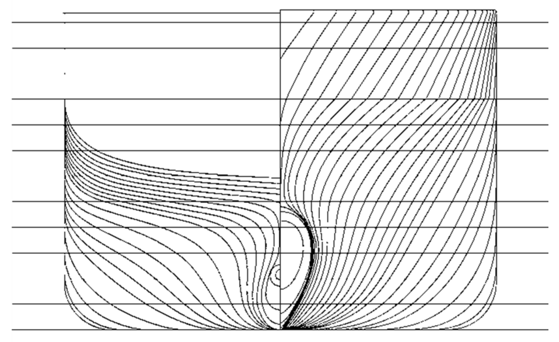
2 emissions. The design speed of KCS corresponds to 22 kn (knots) and the slow steaming speeds range from 18 to 21 kn. The body plan of KCS is presented in Figure 1, and the main particulars are given in Table 1. KCS represents a typical container ship and a benchmark commonly used in numerous studies related to computational fluid dynamics (CFD) [21,22,
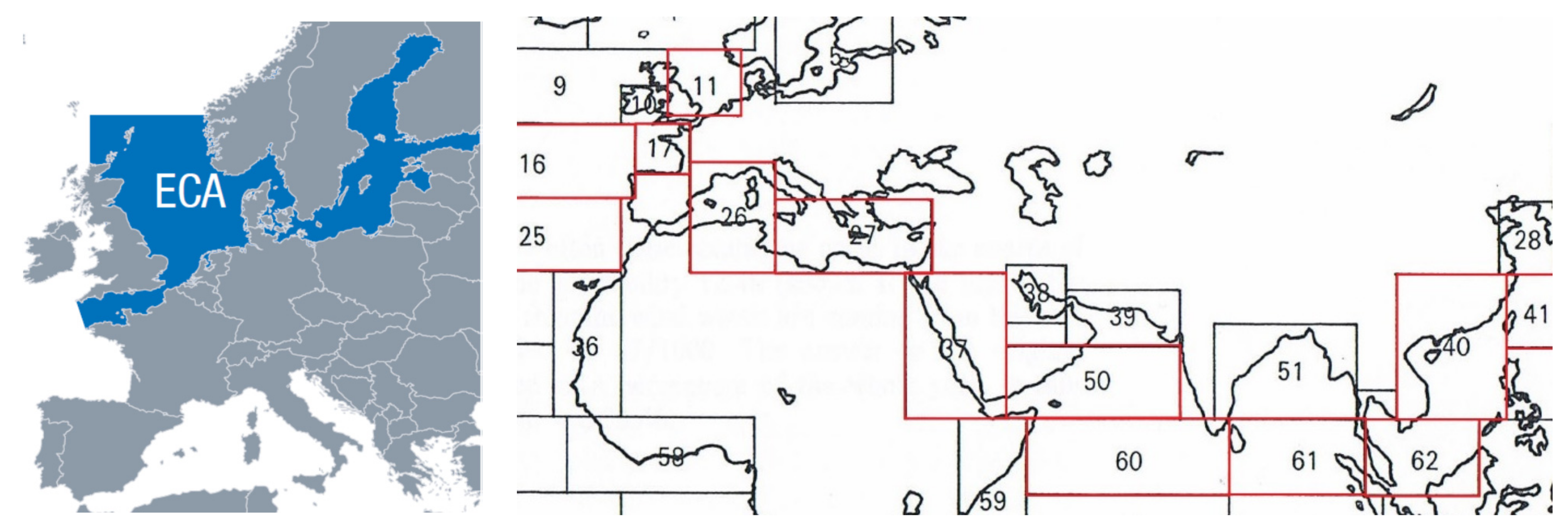
23]. The container ship sailing route connects China (Shanghai port, φ S = 31.303° N, μ S = 121.667° E) and Germany (Hamburg port, φ H = 54.542° N, μ H = 9.915° E) passes through the Mediterranean Sea and is selected for the case study, Figure 2.
Numerical simulations of resistance and self-propulsion tests are carried out utilizing STAR-CCM+. The total resistance of a ship in calm water at the design and slow steaming speeds is obtained in resistance tests, while ship propulsion characteristics are obtained in self-propulsion tests. The governing equations of the applied mathematical model are the Reynolds averaged Navier–Stokes (RANS) equations and the averaged continuity equation [24]:
ρ u ¯ i t + x j ρ u ¯ i u ¯ j + ρ u i u j ¯ = p ¯ x i + τ ¯ i j x j ,
ρ u ¯ i x i = 0 ,
where ρ is the fluid density, u ¯ i is the averaged Cartesian components of the velocity vector, ρ u i u j ¯ is the Reynolds stress tensor, p ¯ is the mean pressure, and τ ¯ i j is the mean viscous stress tensor.
To close the set of Equations (1) and (2), the k ω shear stress transport turbulence model is applied. The size of the computational domains and the boundary conditions applied on the domain boundaries in the numerical simulations of resistance and self-propulsion tests are the same as is [19], while details on the discretization schemes, mesh refinements, time steps, and stopping criteria are explained in [25,26].
Ship total resistance and propulsion characteristics in calm water are validated against the experimental data available in the literature, and the highest relative deviation is equal to 4.58% for relative rotative efficiency [26]. Ship-added resistance in regular head waves is obtained by the boundary integral equation method (BIEM) [27], and the highest relative deviation from the experimental data is equal to 8.6% [11]. The added resistance for sea states with the highest probability of occurrence on the analyzed sailing route [28] is obtained by means of the spectral analysis using the Bretschneider sea spectrum:
S ς ω = H S 2 4 π 2 π T z 4 ω 5 exp 1 π 2 π T z 4 ω 4 ,
where H S is the significant wave height and T z is the zero-crossing period. The term 2 π / T z corresponds to zero-crossing frequency. The areas of the investigated sailing route are shown in Figure 2, and sea states with the highest probability of occurrence are presented in Table 2.
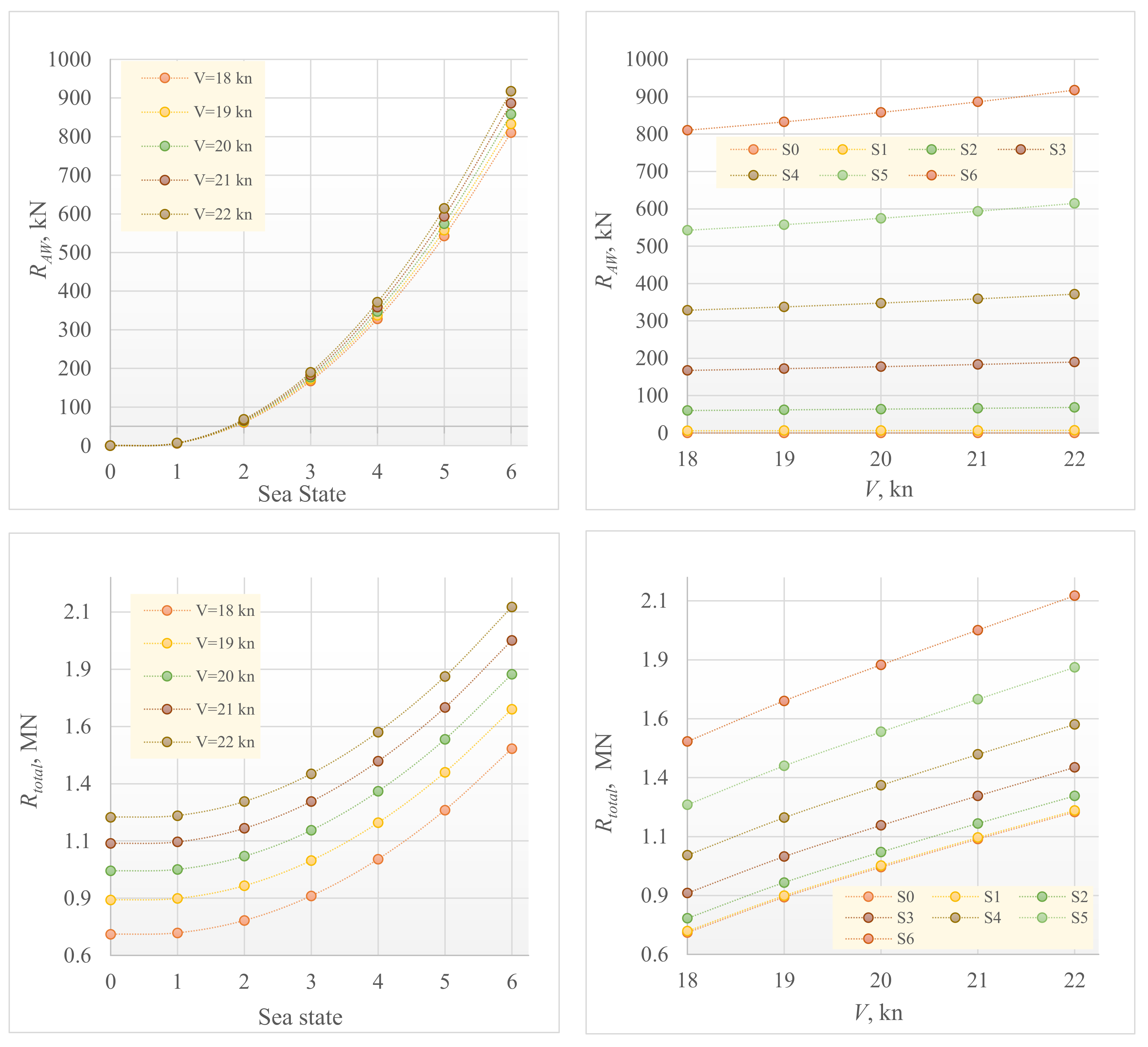
The total resistance in waves is calculated as the sum of calm water resistance R T and added resistance in waves R A W , as follows:
R T O T = R T ( v S ) + R A W ( v S , S I S ) ,
The thrust deduction fraction t , wake fraction w , and relative rotative efficiency η R are obtained in the numerical simulations of the self-propulsion tests in calm water and are assumed to be constant at a certain ship speed for all analyzed sea states.
Based on the thrust deduction fraction depending on ship speed, t ( v S ) , the required thrust in waves is determined by the following equation:
T P = R T O T ( v S , S I S ) 1 t ( v S ) ,
The required thrust depending on the thrust coefficient K T is defined as follows:
T P = K T ( J ) ρ n 2 D 4 ,
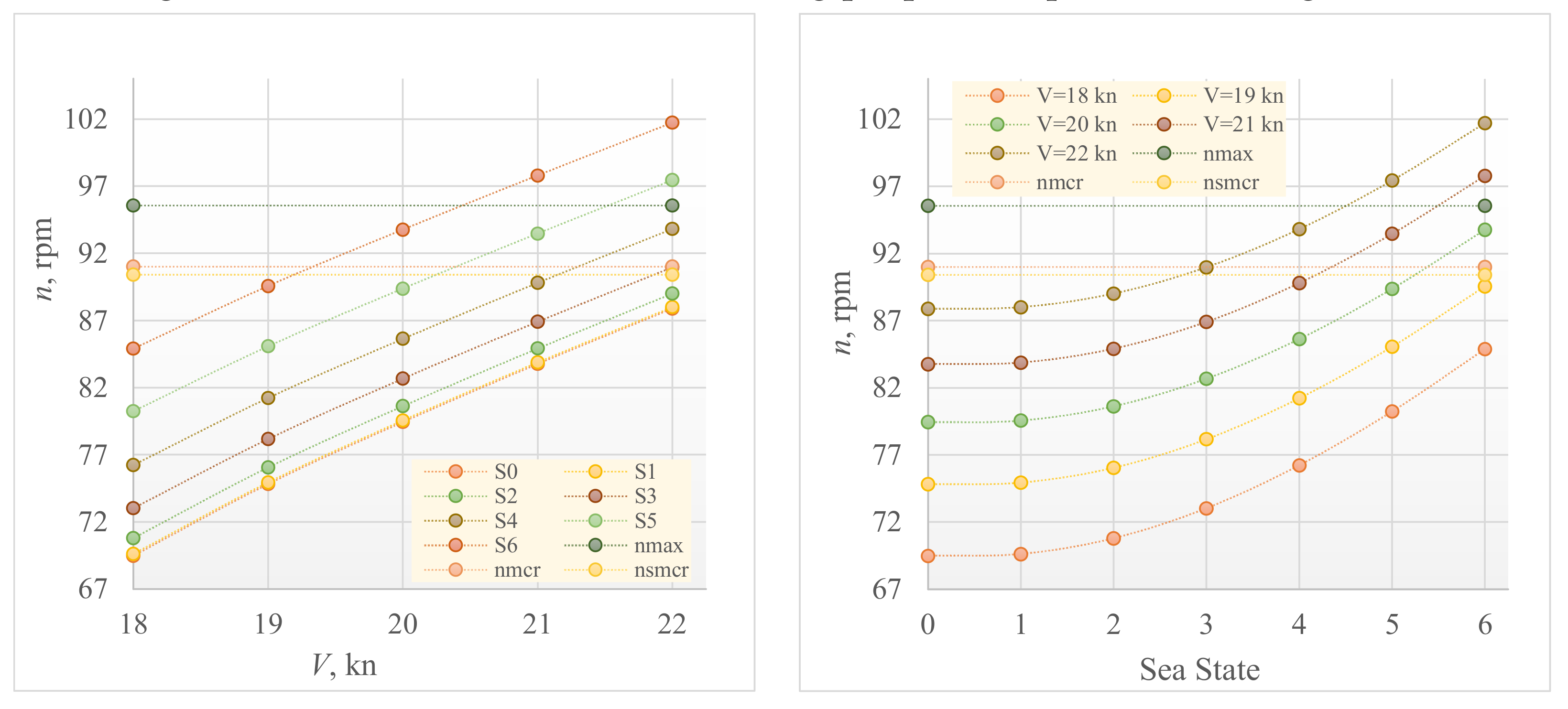
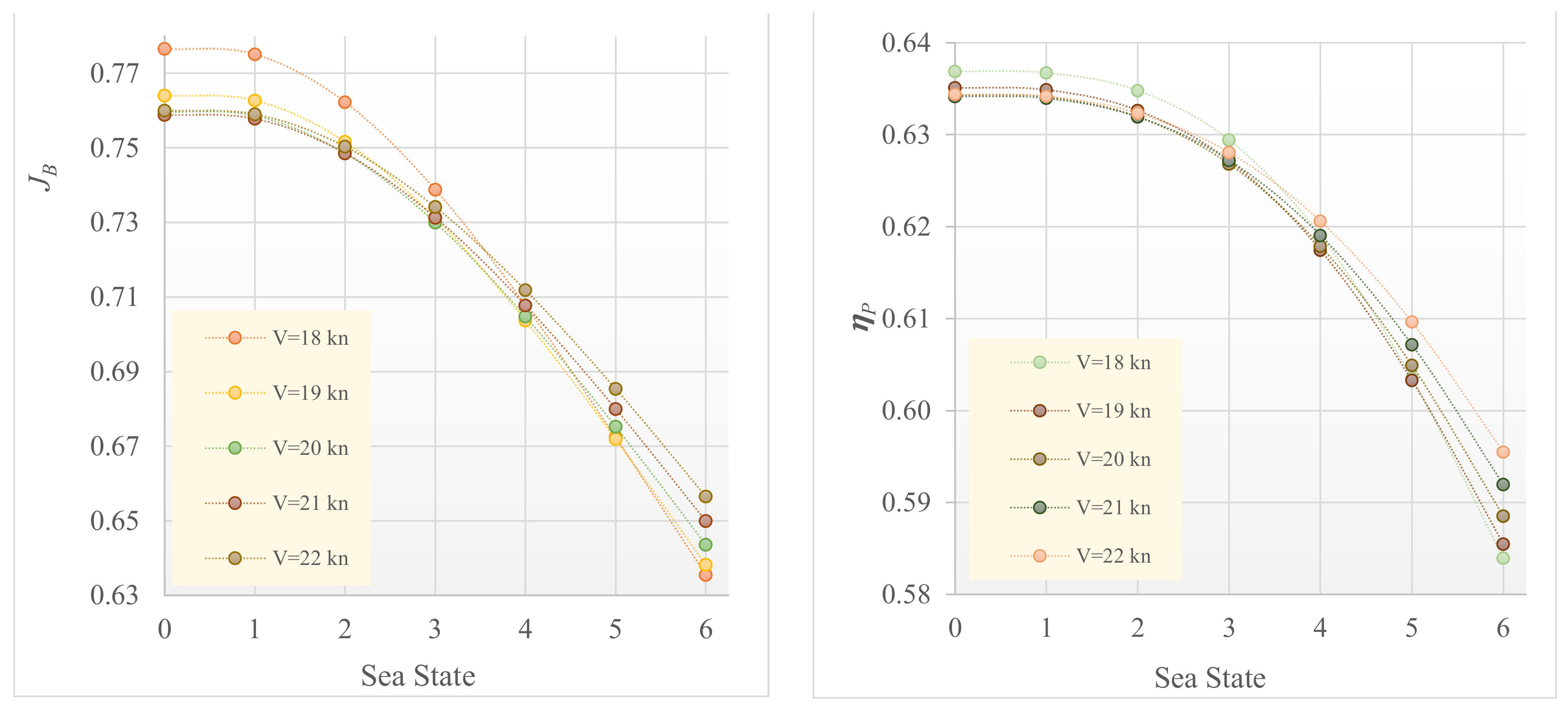
The balancing rate of revolution n B is calculated for each ship speed and sea state, i.e., n B = n B ( v S , S I S ) . Based on the calculated n B = n B ( v S , S I S ) , other propulsion parameters, such as the propeller advance ratio J B ( v S , S I S ) and torque coefficient 10 K Q B ( v S , S I S ) are determined, as well as propeller efficiency η P . Finally, the balancing value of the engine torque, taking into account the propeller shafting efficiency η P S = 0.98 , and the balancing value of brake power are calculated by the following expressions, respectively:
Q B = K Q B ( v S , S I S ) η P S η R ( v S ) ρ D 5 n B 2 ( v S , S I S ) ,
P B B ( v S , S I S ) = π K Q B ( v S , S I S ) 30 η P S η R ( v S ) ρ D 5 n B 3 ( v S , S I S ) = R T O T ( v S , S I S ) v S η O P ( v S ) ,
where η O P ( v S ) = η P S η R ( v S ) η H ( v S ) η P ( v S ) and η H ( v S ) = ( 1 t ) / ( 1 w ) are overall propulsion efficiency and hull efficiency, respectively.

2.2. Selection Procedure for the Main DF Engine Complying with IMO Regulations

Considering the decarbonization trends in maritime transport, the DF engine is currently the most favorable choice. According to MAN propulsion DF engine project guide program [29,30], these engines can run in three fueled modes: FO only; mainly NG with a very small share of the pilot fuel oil (PFO), i.e., 0.5 ÷ 1.5 % of the overall fuel energy income; and fuel-sharing mode (FSM), also referred to as specified dual fuel (SDF) mode, where the ratio between PFO and NG can be selected according to preset values.
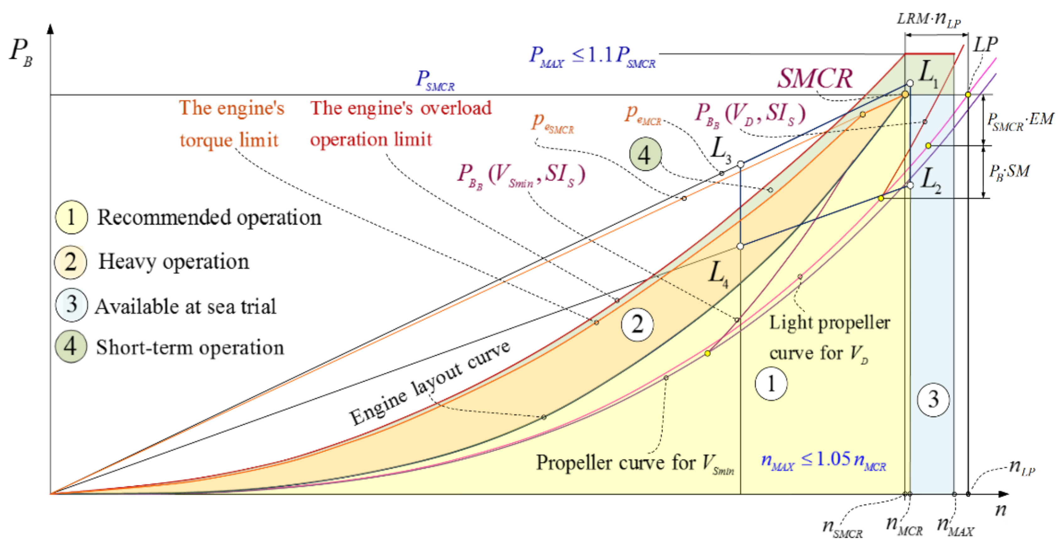
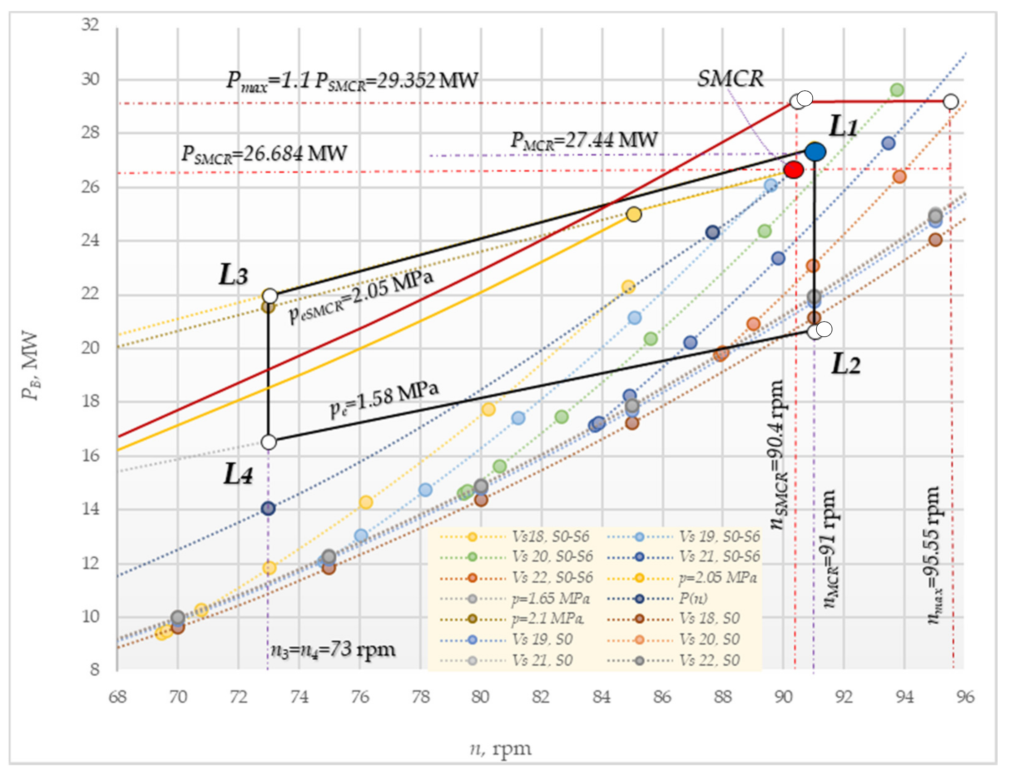
The selection DF engine is based on the fact that SMCR (specified maximum continuous rating) must be located within the engine layout diagram (inside of the quadrangle defined by points L1, L2, L3, and L4), Figure 3. For the SMCR, corresponding break power P S M C R and the rate of revolution n S M C R are calculated as follows:
P S M C R = P D 1 + S M 1 E M ,
n S M C R = n L P ( 1 L R M ) ,
where S M = 0.1 ÷ 0.2 and E M = 0.1 ÷ 0.15 are sea and engine margine, respectively, while L R M = 0.04 ÷ 0.07 is light running margine.
Further, n L P is the rate of revolution at the light propeller (LP) curve that is calculated for P L P = P S M C R as follows:
n L P = n D P S M C R P D 1 / 3 ,
Since SMCR must be within the engine layout diagram, n S M C R must be greater than:
n S M C R n M C R P S M C R P M C R ,
Because part of the analyzed sailing route passes through ECAs (emission control area), Figure 2, the selected DF engine complies with IMO’s Tier II and Tier III (for ECAs) regulations. It should be noted that Tier II refers to non-ECAs (in the rest of the paper moderate ECAs, MECAs), where according SOx rules [31] mass sulfur fraction in FO and PFO must be s 0.5 % , while Tier III refers to ECAs with mass sulfur fraction s 0.1 % . Consequently, inside ECAs DF engines must be fueled by the ultra low sulfur fuel oil (ULSFO) with s U L S F O 0.1 % , and outside ECAs (MECAs) by the very low sulfur fuel oil (VLSFO) with s V L S F O 0.5 % . In general, both ULSFO and VLSFO can be either marine gas oil (MGO), distillate (DM), or residual (RM) marine fuels.
On the other hand, according to the NOX rules, for ECAs Tier III requirements must be applied for NOx reductions on two-stroke DF engines, which can be fulfilled by two alternative methods: EGR (exhaust gas recirculation) and SCR (selective catalytic reduction). Both alternative methods have two emission-cycle operating modes: Tier II for operation outside NECAs (NOX ECAs) and Tier III for operation inside NECAs.
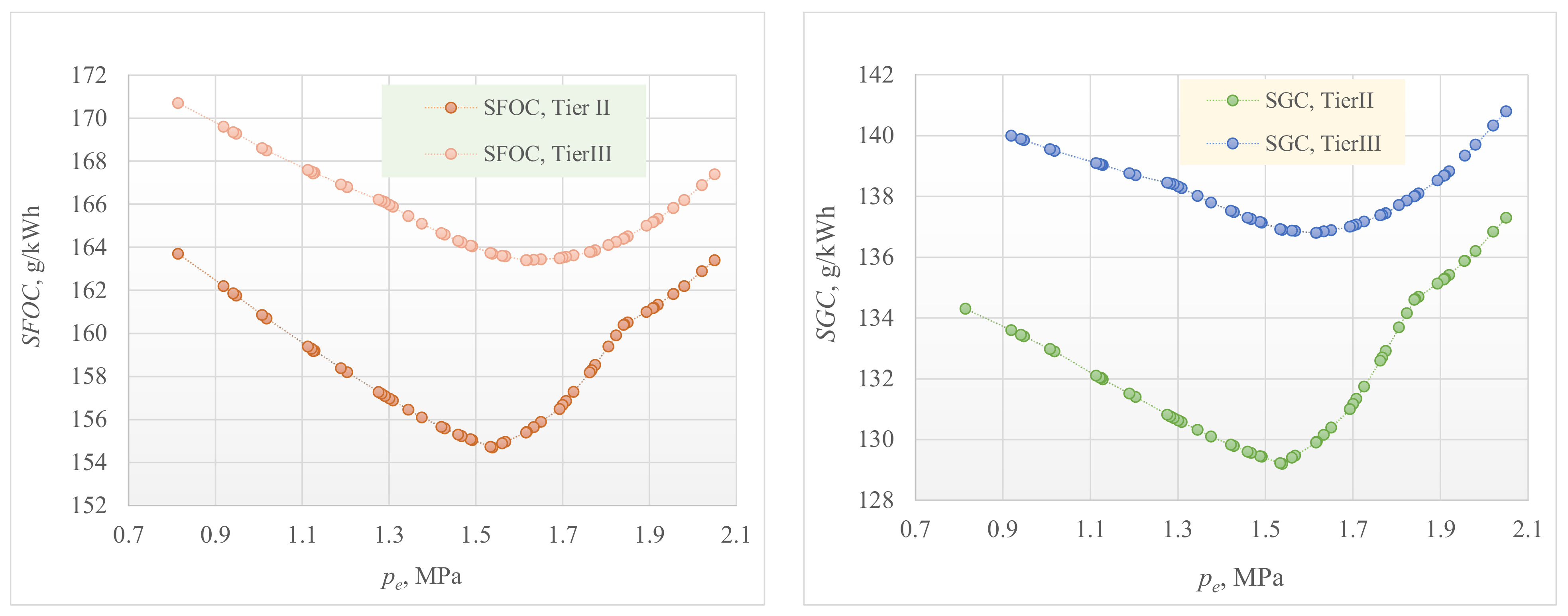
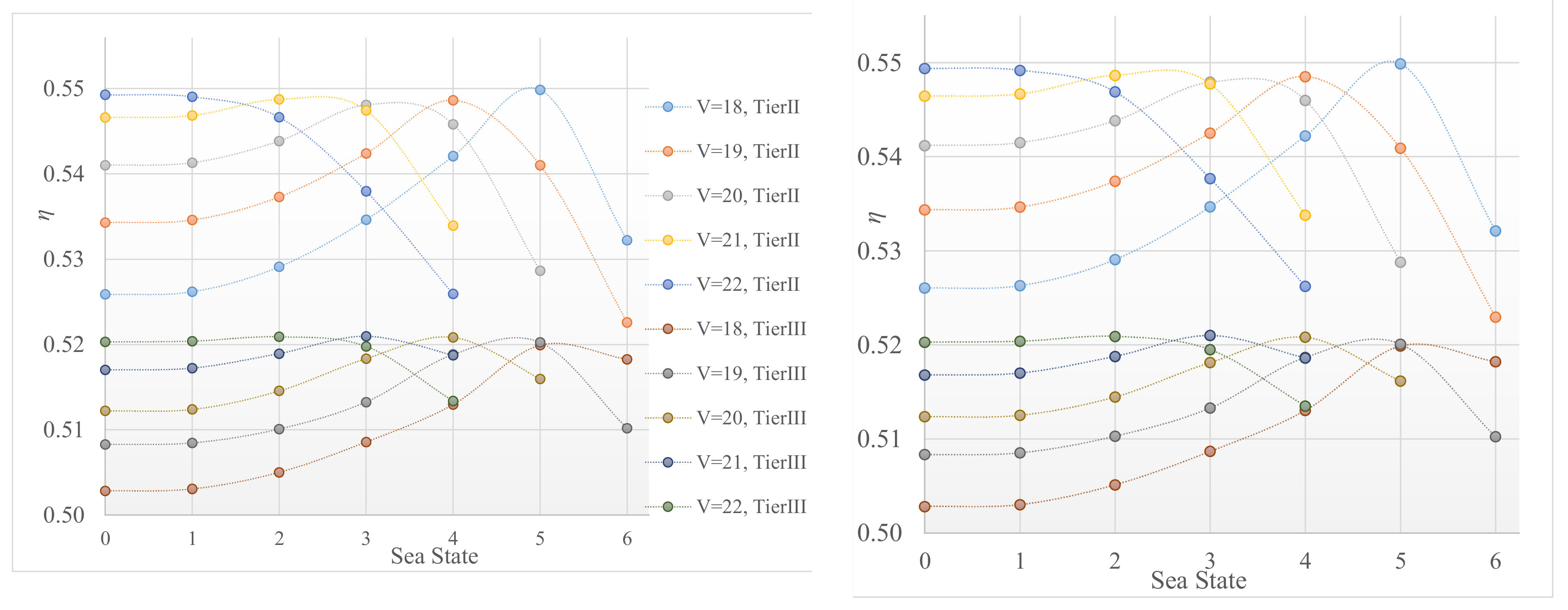
For sailing at the design and slow steaming speeds, with the determined SMCR of the selected engine, four optimization variants, concerning the reduction in the specific fuel oil consumption (SFOC) and consequently CO2 emissions, have been conducted using the MAN computerized engine application system (CEAS). These variants include FO and NG modes complying with Tier II and Tier III regulations (TR-Tier Regulations). In the remaining part of the paper, Tier II and Tier III are indexed by II and III, respectively.
The energy efficiencies for selected fueling mode (FM), depending on the specific fuel consumption at specified TR S F C F M , T R ( p e B ) , are determined for NG and FO modes as follows:
η N G , T R ( p e B ) = 3600 S P O C T R ( p e B ) L H V F O + S N G C T R ( p e B ) L H V N G ,
η F O , T R ( p e B ) = 3600 S F O C T R ( p e B ) L H V F O ,
where S F O C T R ( P B B ) , S P F O C T R ( P B B ) , and S N G C T R ( P B B ) are specific consumptions of FO, PFO, and NG in a TR mode, respectively, and L H V F O and L H V N G are lower heating values for FO and NG, respectively.
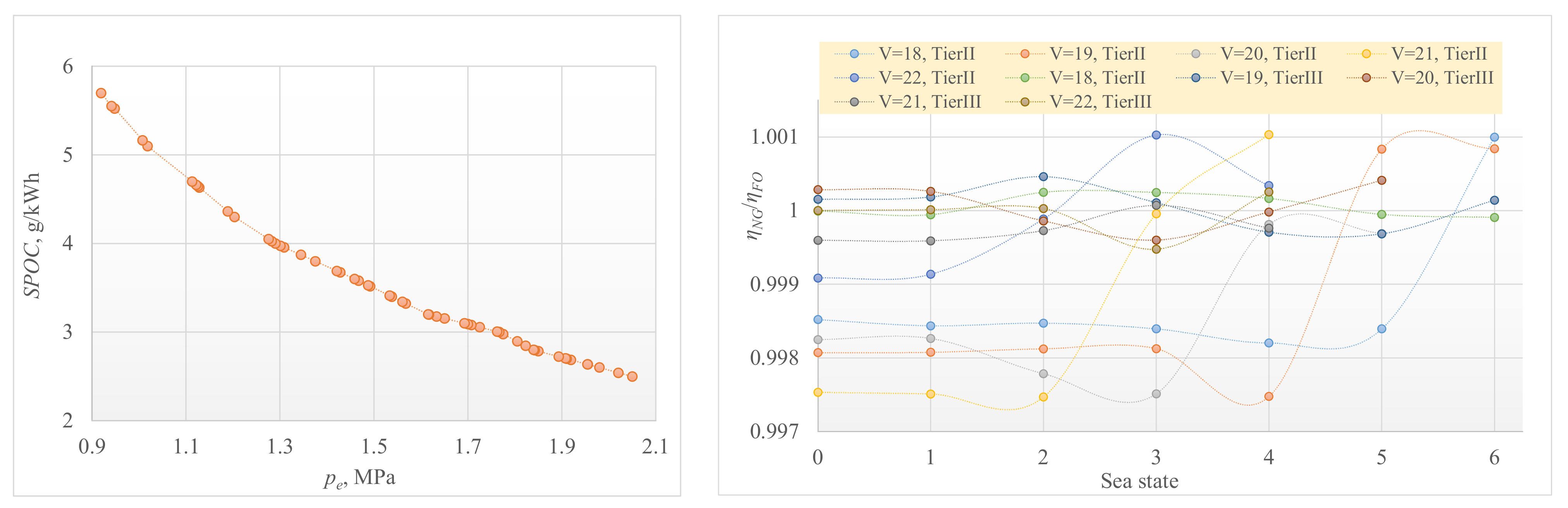
Based on the S F C F M , T R ( p e B ) 
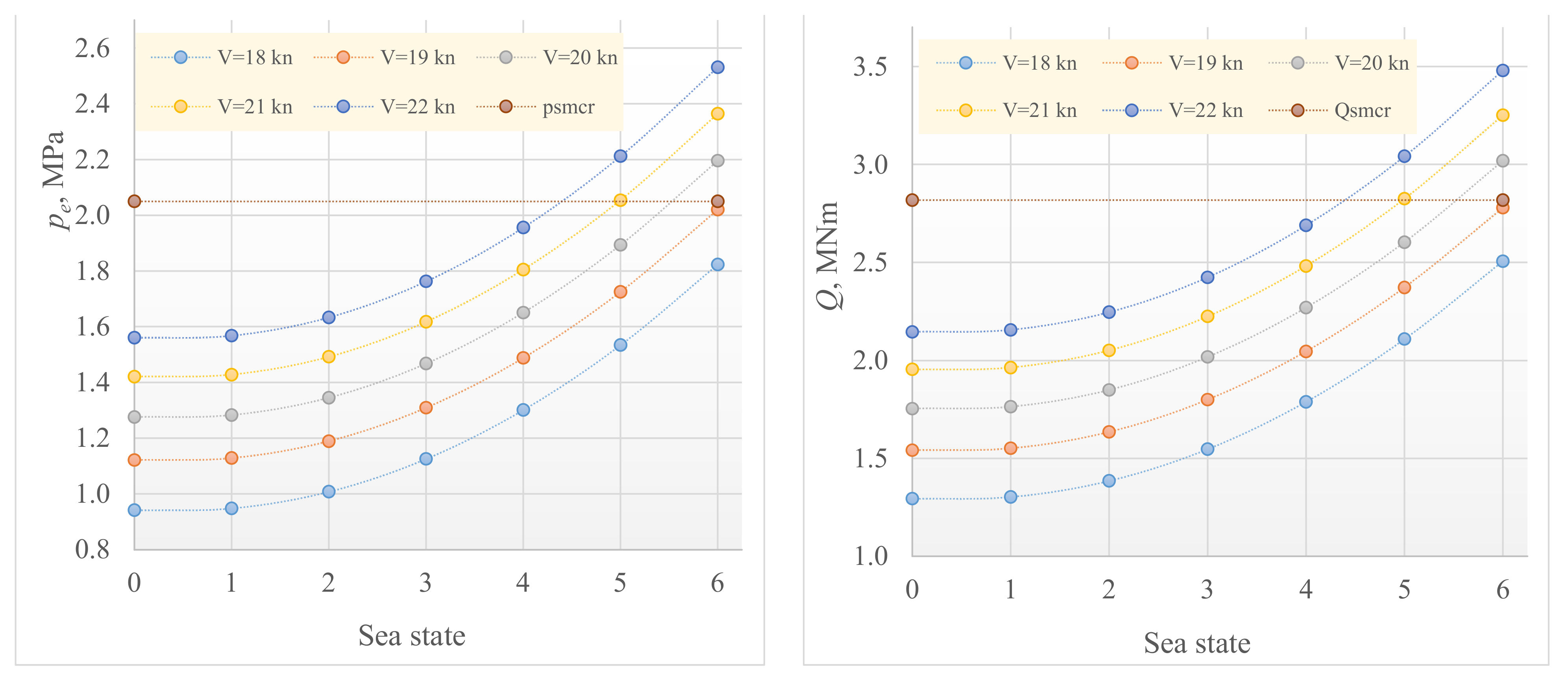
values for the operating scenarios obtained using the CEAS, the fuel consumptions (FC) such that FOC (FO consumption), PFOC (pilot FO consumption), NGC (NG consumption), and 
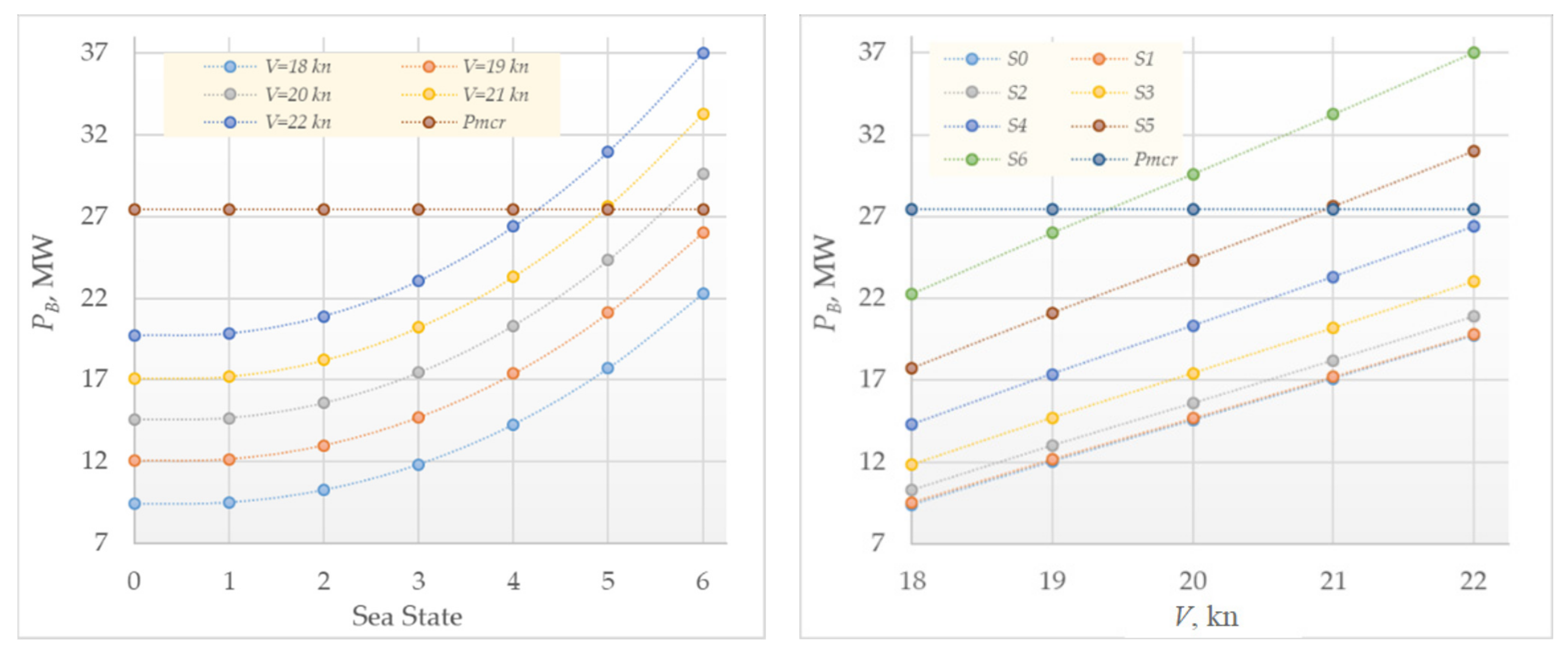
CDE (carbon dioxide emission), depending on the both balancing mean effective pressure p e B ( v S , S I S ) and brake power P B B = P B B ( v S , S I S ) , can be calculated using the following equations:
F C ( v S , S I S ) F M , T R = S F C ( p e B ) F M , T R P B B ( v S , S I S ) T R ,
C D E ( v S , S I S ) F M , T R = S F C ( p e B ) F M , T R C F F M , T R P B B ( v S , S I S ) T R ,
where C F F M , T R represents stoichiometric factors depending on the selected FM at specified TR.

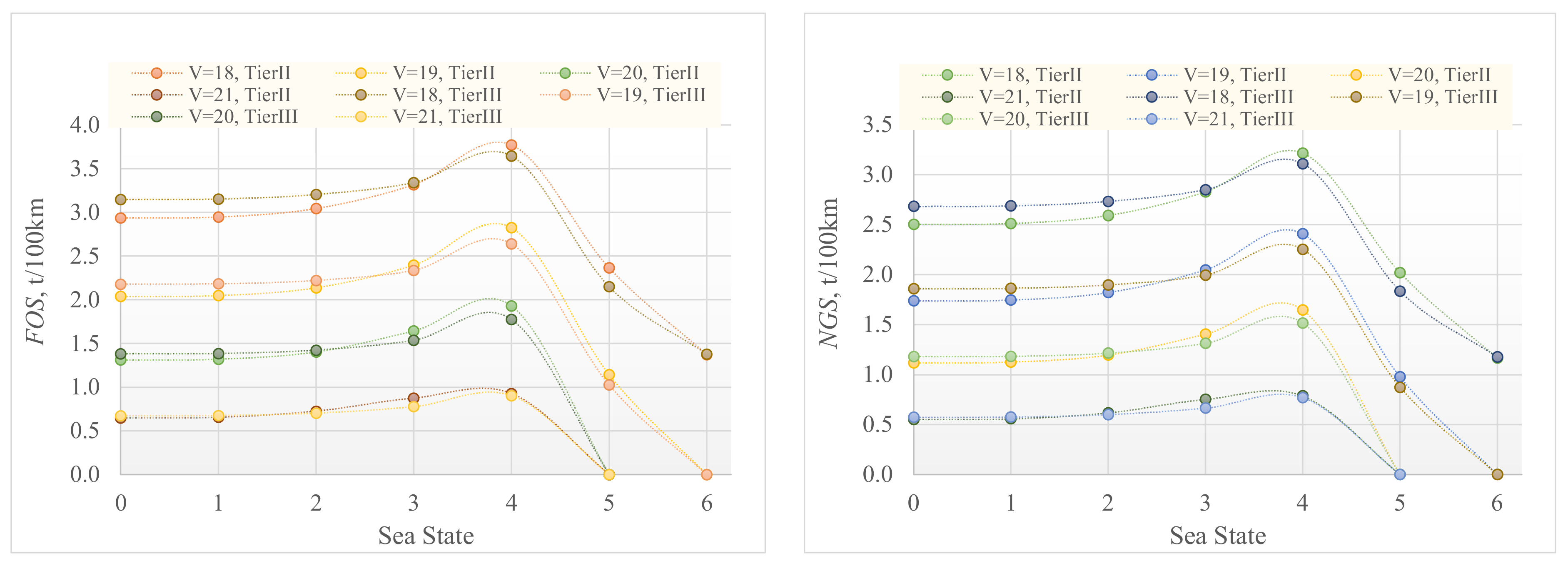
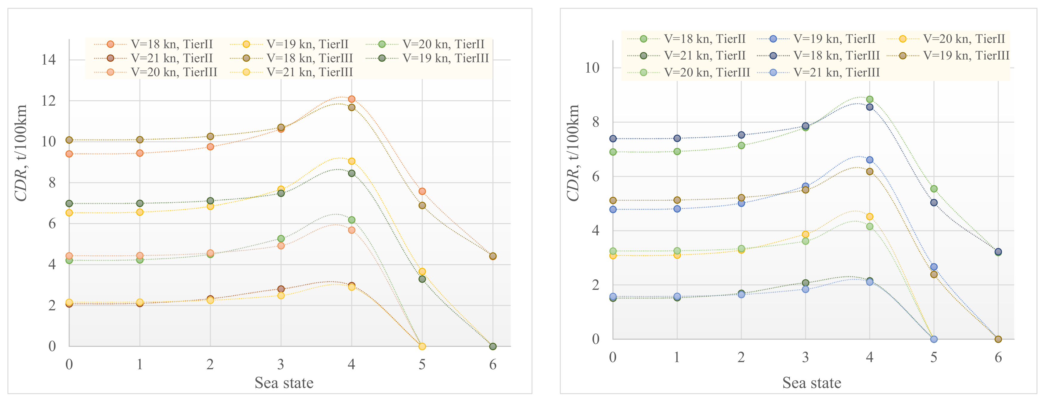
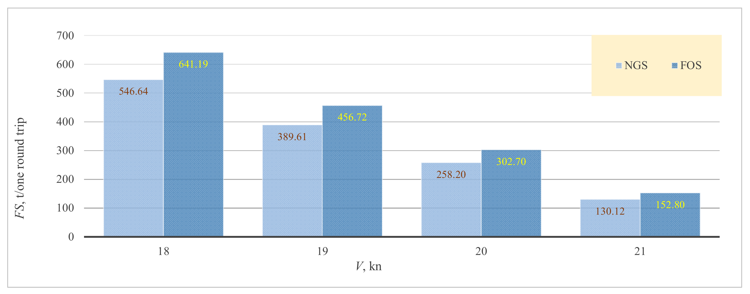
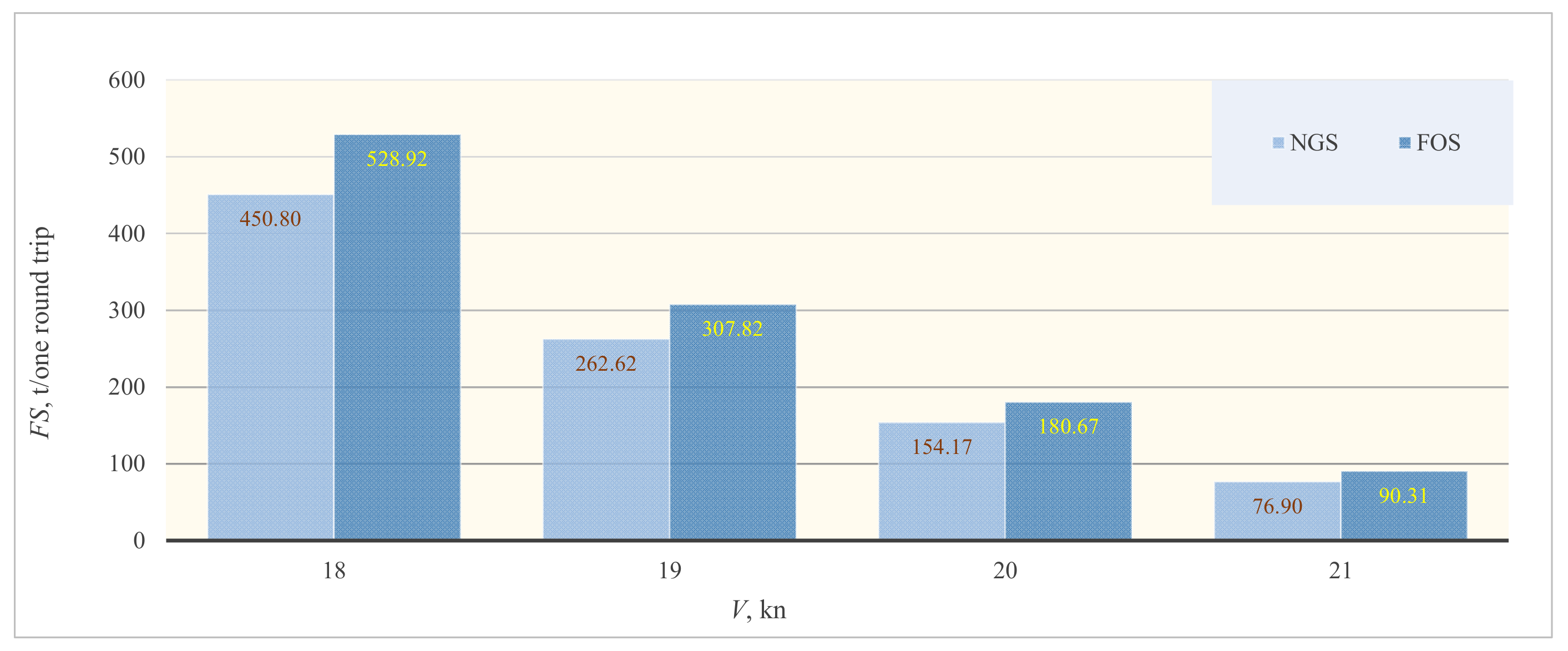
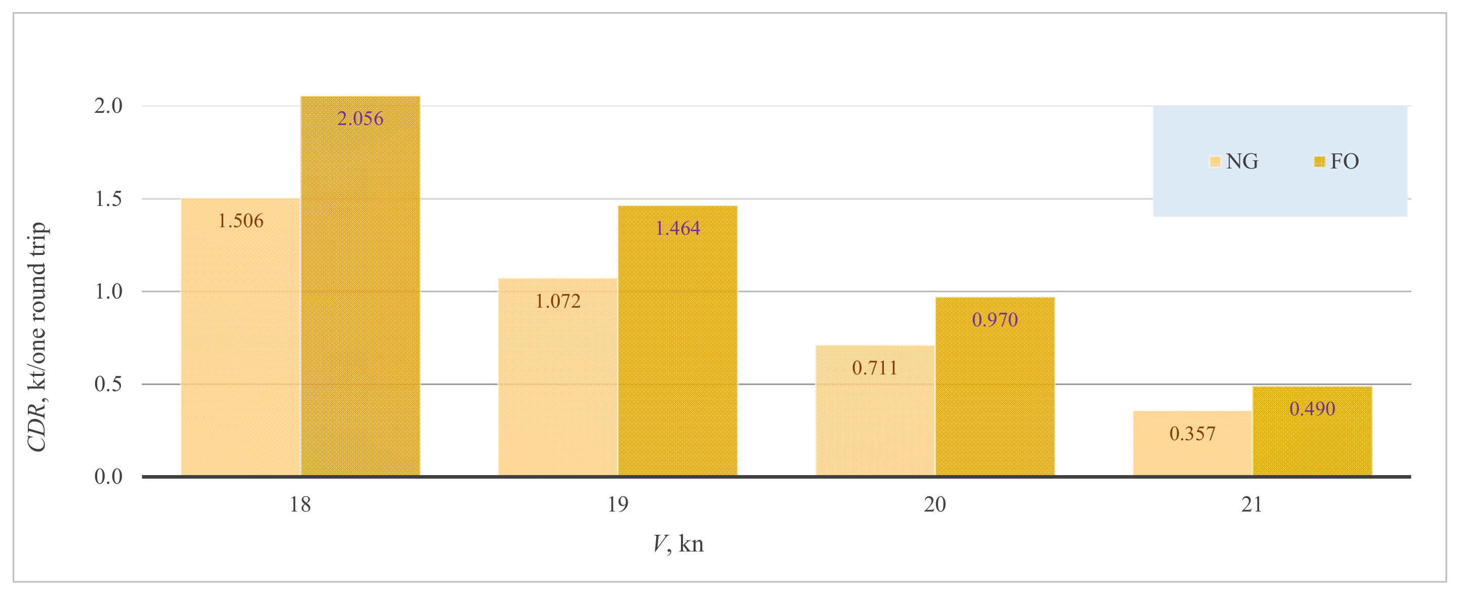
2.3. Fuel Savings and CO2 Emission Reduction

Finally, the fuel savings (FS) and carbon dioxide reduction (CDR), per one kilometer of the sailing route in selected FM at specified TR, for the slow steaming speeds are calculated as follows:
F S ( v S , S I S ) F M , T R = F C ( v S n a x , S I S ) F M , T R v S max ( S I S ) T R F C ( v S , S I S ) F M , T R v S ,
C D R ( v S , S I S ) F M , T R = C D E ( v S max , S I S ) F M , T R v S max ( S I S ) T R C D E ( v S , S I S ) F M , T R v S ,
where S I S corresponds to the sea state within TR areas, v S max ( S I S ) I I , I I I v D is the maximum attainable sailing speed for the installed propulsion system, and v S is slow steaming speed. It should be noted that F S ( v S , S I S ) F M , T R and C D R ( v S , S I S ) F M , T R are calculated concerning the maximum attainable sailing speeds in realistic sailing conditions defined by sea states expected in each segment of the sailing route.
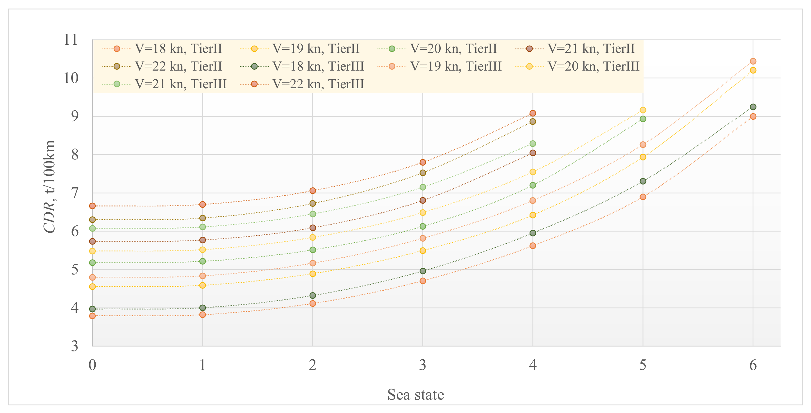
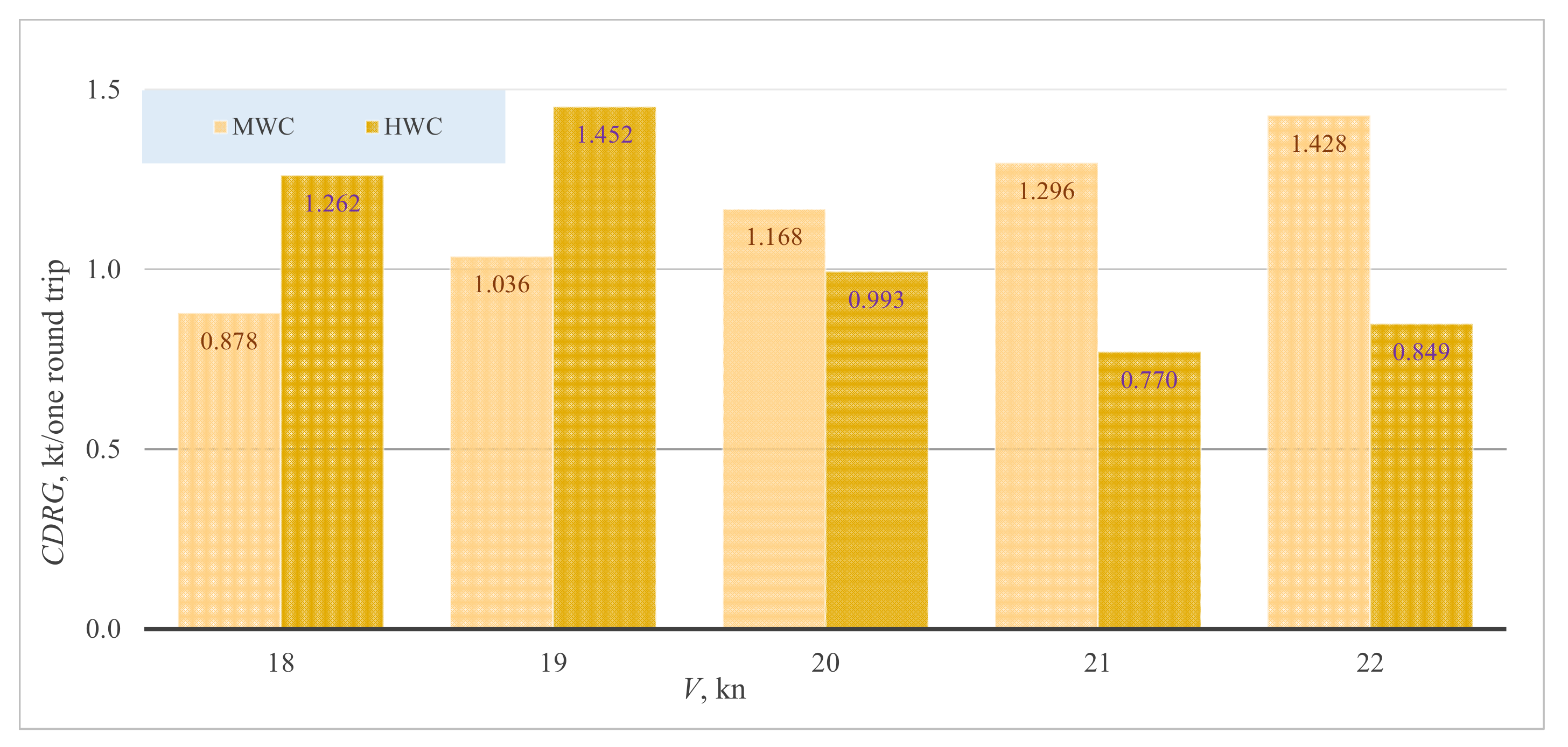
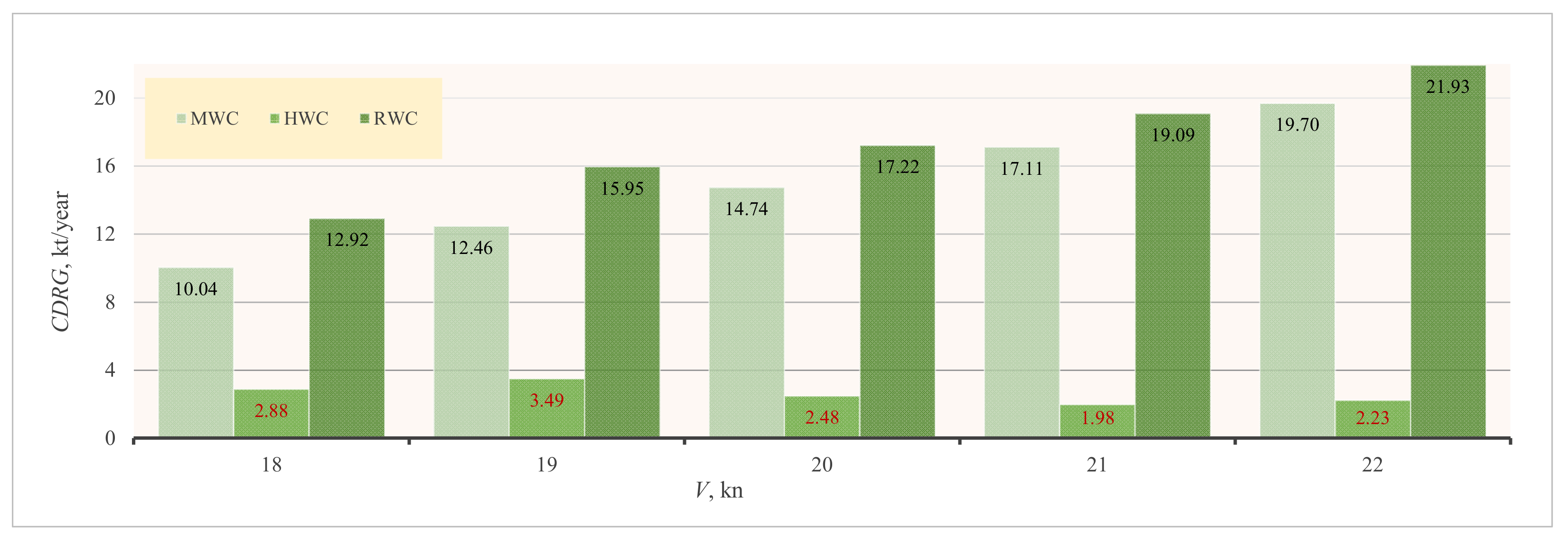
Additionally, the gasification effects on CDR are considered for the ecological valorization of the container ship powered by NG compared to the one powered by FO. Therefore, the corresponding CO2 emission reduction (CDRGCDR for gasification) for slow steaming speeds is calculated as follows:
C D R G ( v S , S I S ) T R = C D E ( v S , S I S ) F O , T R C D E ( v S , S I S ) N G , T R v S ,
The yearly fuel savings ( F O S Y , P F O S Y , and N G S Y ) and CO2 emission reductions( C D R F O , Y , C D R N G , Y , and C D R G Y ) greatly depend on the engine’s load profile, which is rather predictable because container vessels typically navigate by schedule with transoceanic crossings. For a ship to arrive at the port on time, it is important to maintain a schedule, which sometimes requires operation at higher loads than usual, especially during navigation under harsh weather conditions. Therefore, it is necessary to predict the sea states that will occur during moderate and harsh weather conditions.
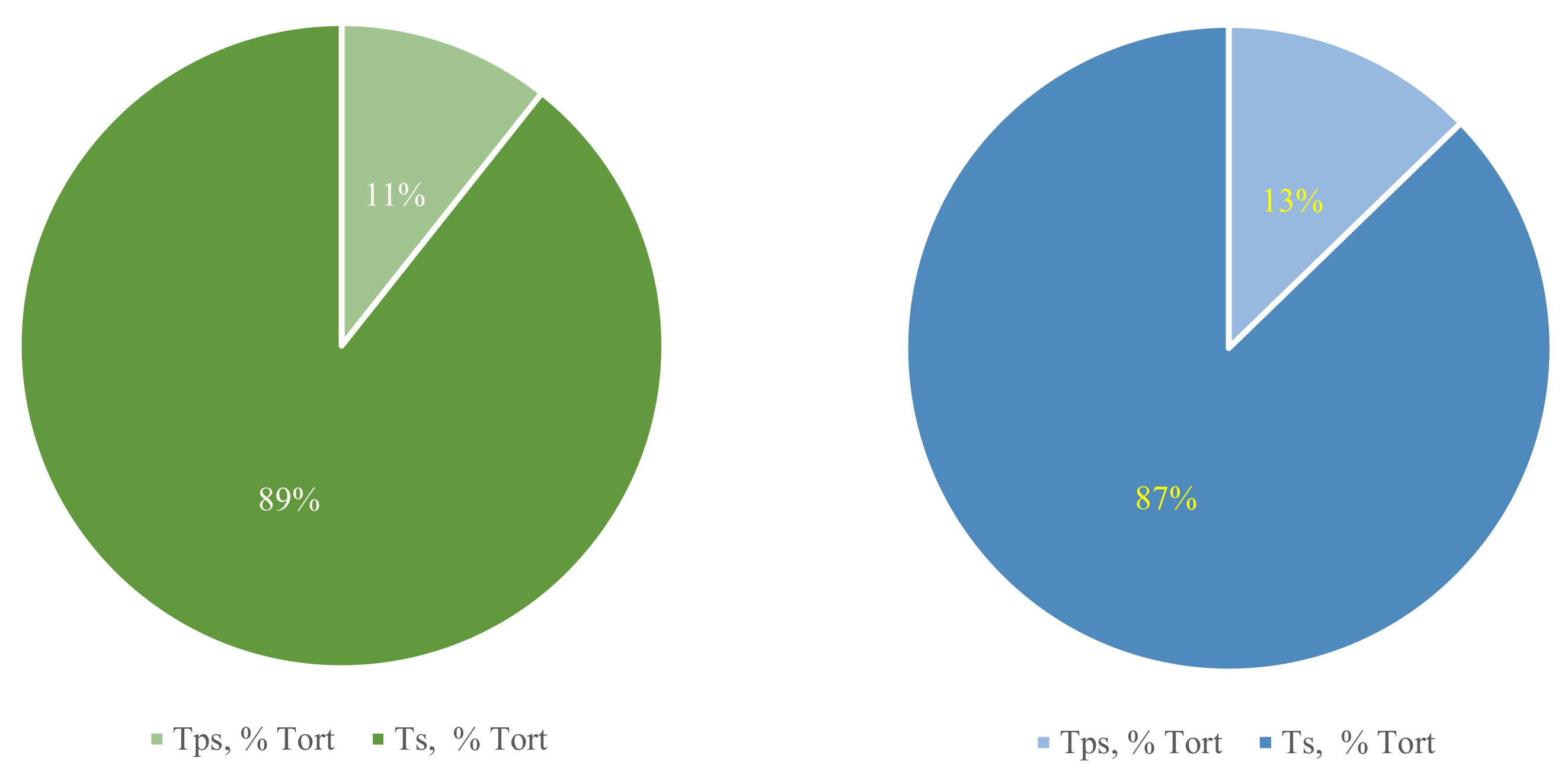
In general, the time interval of one transport cycle between two terminals τ O R T (one round trip) contains time intervals of the ship being at berth τ P S (loading and unloading intervals, so-called port staying time), and two navigation intervals τ O T depending on the ship loading condition (so-called one trip). It should be noted that the effects of a ship being at berth and during its maneuvering on the fuel consumption and CO2 emission have been ignored since fuel consumption and CO2 emissions are the most conspicuous during the sail [32]. In further analysis, navigation intervals in a full loading condition are considered only, taking into account different IMO regulations for certain parts of the sailing route.
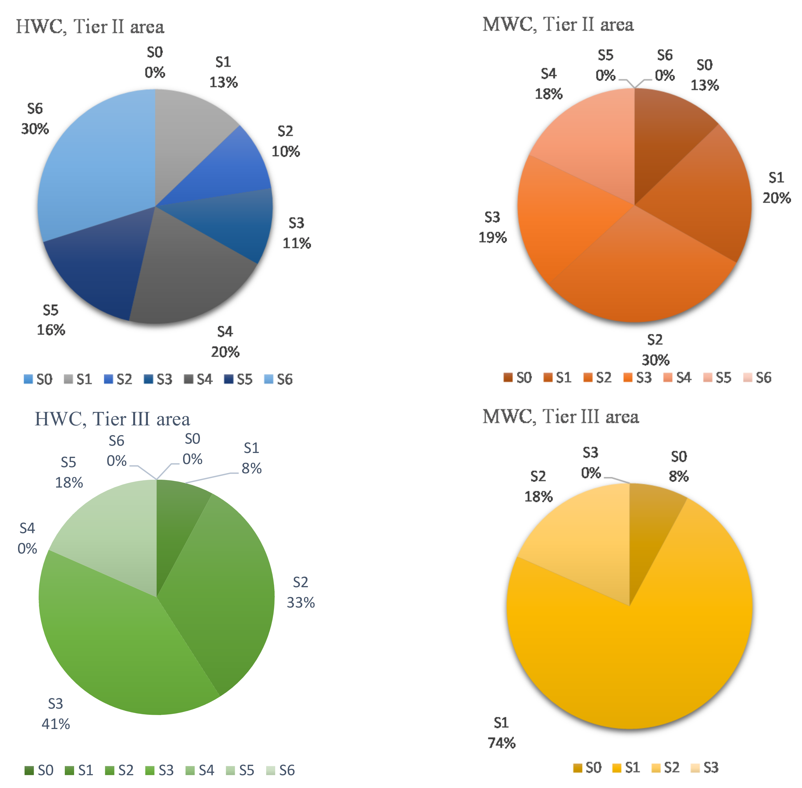
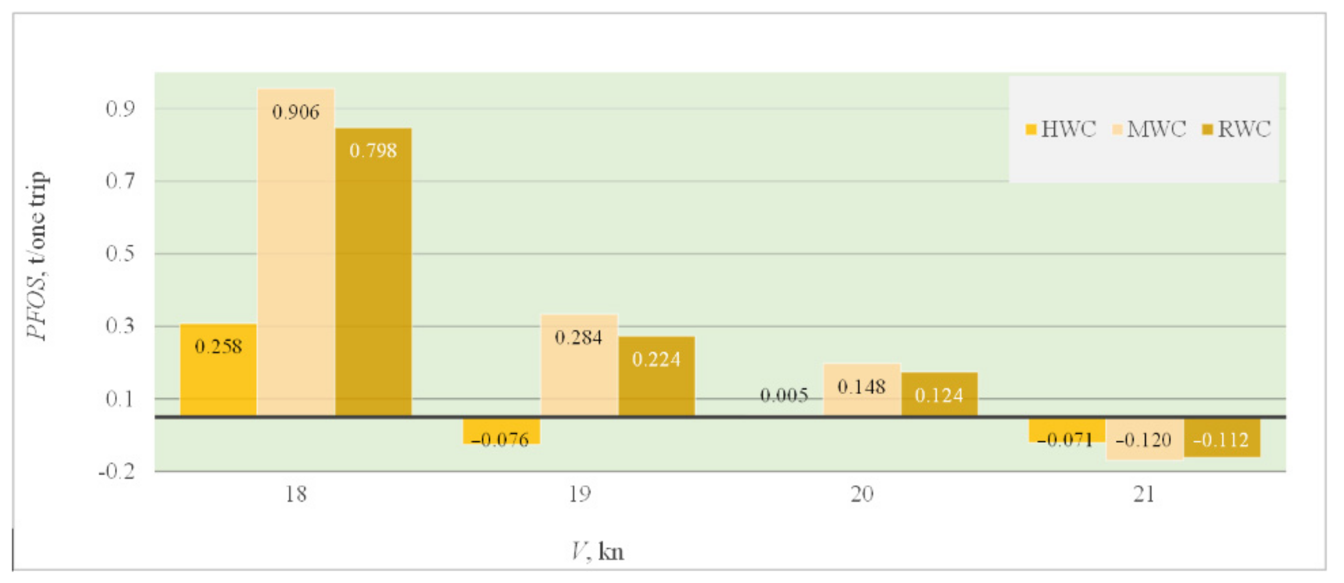
Furthermore, based on the realistic environmental conditions that can be experientially predicted based on logbooks for container ships on the particular sailing route, the overall sailing route can be divided into segments with respect to the sea states that will occur during one year. In that context, the occurrence of moderate (MWC) and harsh weather conditions (HWC) is defined for the analyzed sailing route, denoted as S I M W C and S I H W C for moderate and rough sea states, respectively.
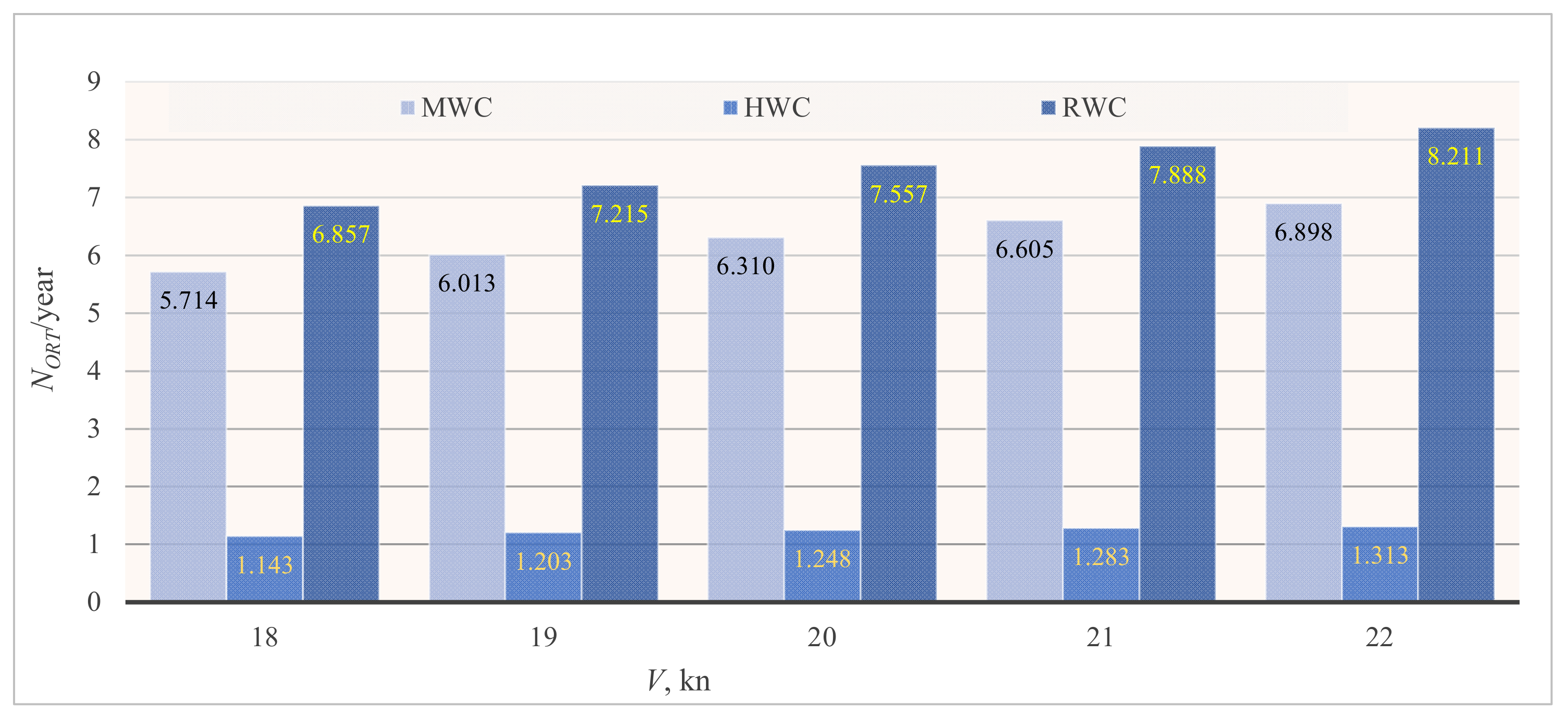
The total number of round trips per year N O R T , depending on the assumed weather conditions defined by the weather conditions factor f W C and slow steaming speed, is determined as follows:
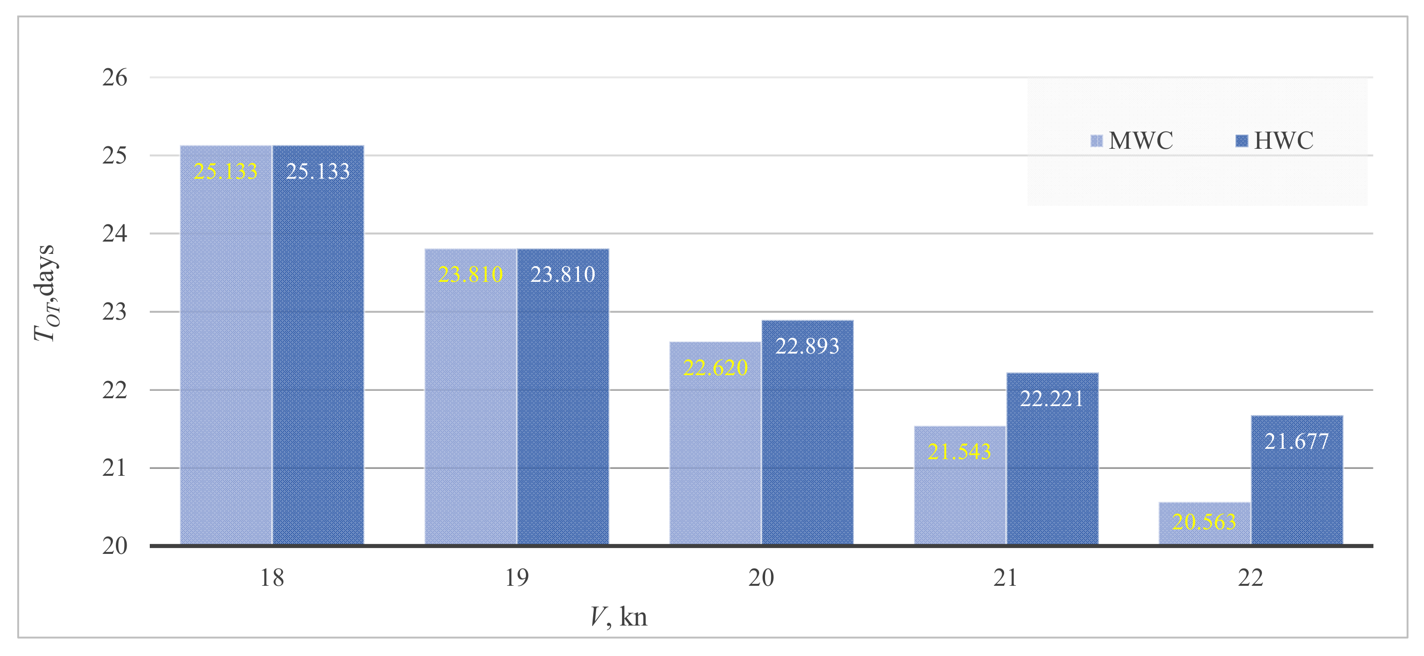
N O R T = τ S Y τ O R T ( v S , f W C ) = τ S Y 2 τ P S + τ O T ( v S , f W C ) ,
where τ S Y = 365.25 days is the number of days of the sidereal year, τ P S is the port staying time, and τ O T ( v S , f W C ) is the sailing time between ports, which depends on the ship speed v S and appearing f W C .
Taking into account the predicted time intervals τ H W C of the HWC and τ M W C of the MWC, f W C is defined as f W C = τ H W C / τ S Y = 1 τ M W C / τ S Y .
By assuming that there are no constraints for attainable sailing speed (up to the design speed) under MWC, N O R T for one realistic operating profile of a ship is defined as follows:
N O R T = N O R T ( v S , S I M W C ) + f W C τ S Y 1 τ O R T H W C ( v S , S I H W C ) 1 τ O R T M W C ( v S , S I M W C ) ,
where N O R T ( v S , S I M W C ) is the number of ORT per year under MWC, and it is defined as follows:
N O R T ( v S , S I M W C ) = τ S Y τ O R T M W C ( v S , S I M W C ) ,
The times required for one trip under MWC and HWC, τ O T M W C and τ O T H W C , respectively, are defined as follows:
τ O T M W C ( v S , S I M W C ) = L T O T v S ( S I M W C ) ,
τ O T H W C ( v S , S I H W C ) = L T O T v S ( S N F S ) + I C S = ( 1 + N F S ) N C S L I C S v max ( S I C S ) v S ( S N F S ) ,
where L T O T is the total length of a route, L I C S is the length of the part of the route with extreme sea states under HWC constraining the design sailing speed S I C S , S N S F is the highest sea state that does not constrain the sailing speed, N F S is the number of sea states that do not constrain the sailing speed, N C S is the number of sea states under HWC limiting sailing speed ( N C S > N F S ), v S ( S I F S ) is the sailing speed without constrains for all S I F S S I C S , and v max ( S I C S ) is the maximum attainable sailing speed for L I C S .
To calculate the fuel savings ( F O S O T , P F O S O T , and N G S O T ) and CO2 emission reduction in FO-fueled mode C D R O T , F O and NG-fueled mode C D R O T , N G , and C D R G O T during the one trip and for the specified slow steaming speed v S , the following equations are used:
F S O T ( v S , S I S ) F M = j I I = 1 n I I F S ( v S , S I S ) F M , I I L j I I + j I I I = 1 n I I I F S ( v S , S I S ) F M , I I I L j I I I ,
C D R O T ( v S , S I S ) F M = j I I = 1 n I I C D R ( v S , S I S ) F M , I I L j I I + j I I I = 1 n I I I C D R ( v S , S I S ) F M , I I I L j I I I ,
C D R G O T ( v S , S I S ) = j I I = 1 n I I C D R G ( v S , S I S ) L j I I + j I I I = 1 n I I I C D R G ( v S , S I S ) L j I I I ,
where L j I I and L j I I I are lengths of the sailing route segments where S I S occur in MECAs (indexed by II), and ECAs (indexed by III).
Further, to evaluate the length of the sailing route, the route between Shanghai (index S) and Hamburg (index H), assumed to be equal for the westbound and eastbound trip, is divided into n S straight line segments on the geographical map (Mercator chart), Figure 2. Thus, the route length is defined by:
L S H = L H S = i = 1 n s + 1 L i , i + 1 ,
where index i denotes the initial node of the jth route segment, and through that route segment the latitude φ j depends on the longitude μ j and is expressed as follows:
φ j ( μ j ) = φ i + 1 + φ i + 1 φ i μ i + 1 μ i μ j μ i ; φ i φ j ( μ ) φ i + 1 ; μ i μ j μ i + 1 ,
The differential length of the route segment in the Cartesian coordinate system is defined by the d L j = ( d x j ) 2 + ( d y j ) 2 + ( d z j ) 2 , where d x j , d y j , and d z j are contained Cartesian differential segments, thus the length of the route segment L j = L i , i + 1 is defined by the following integral:
L i , i + 1 = r E μ i μ i + 1 d d μ j cos φ j ( μ j ) cos μ j 2 + d d μ j cos φ j ( μ j ) sin μ j 2 + d d μ j sin φ j ( μ j ) 2 d μ j ,
where r E = 6367.5 km is the mean Earth radius (taking into account the average geoid undulation on the sea surface, which is assumed 100 m) obtained by numerical integration.
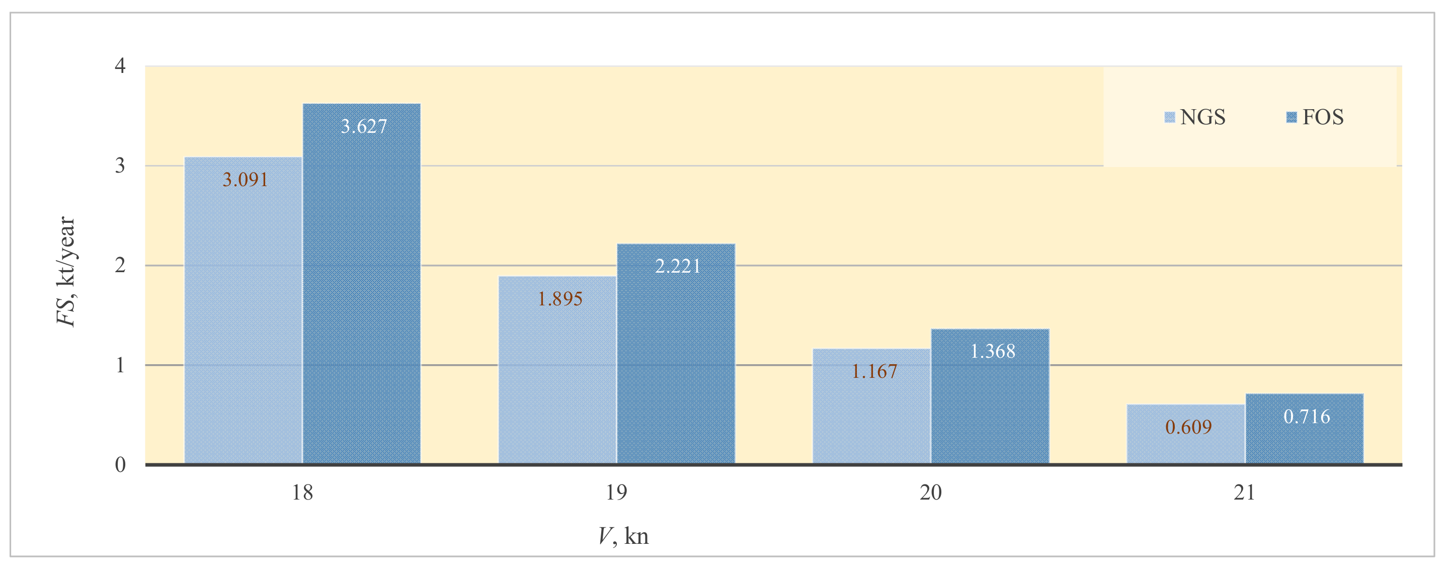
Finally, based on the calculated values of N O R T Y , the total fuel savings and CO2 emission reductions per year for a FO- and NG-fueled ship, can be calculated as follows:
F S Y ( v S , f W C ) F M = 2 N O R T ( v S ,   f W C ) F S O T ( v S , f W C ) FM , t / year ,
C D R Y ( v S , S I S ) F M = 2 N O R T ( v S ,   f W C ) C D R O T ( v S ,   f W C ) F M , t / year ,
C D R G Y ( v S , S I S ) = 2 N O R T ( v S ,   f W C ) C D R G O T ( v S ,   f W C ) , t / year ,
As NG-fueled mode includes simultaneous consumption of PFO and NG, for energy efficiency valorization it is more appropriate to compare total fuel energy consumption in relation to FO mode. For this purpose, the energy efficiency ratio (EER) between FO- and NG-fueled modes for one year is introduced as follows:
E E R = F O C Y ( v S , S I S ) L H V F O P F O C Y ( v S , S I S ) L H V F O + N G C Y ( v S , S I S ) L H V N G ,
Although the economic aspects of slow steaming are not considered within this paper, their impact on the yearly freight income is worth mentioning, which is a key parameter for the evaluation of the economic effects. The freight income efficiencies ratio (FIER) between freight incomes achievable at slow steaming and those achievable at maximum attainable sailing speeds on the sailing route during one year is defined as:
F I E R = N O R T ( v S , S I S ) N O R T ( v S max , S I S ) ,

3. Results and Discussion

3.1. Ship Resistance and Balancing Propulsion Characteristics

The numerical results obtained are presented within this section. The total resistance of a ship in calm water and propulsion characteristics at the design and slow steaming speeds are shown in Table 3.
R T w t η R η H T P The added resistance in regular waves is calculated for sea states with the highest probability of occurrence on the selected sailing route, Table 2, and the results for the added resistance are shown in Table 4. Thereafter, the total resistance in waves is determined as the sum of the total resistance in calm water and the added resistance in waves, Figure 3.
Based on these results, the required thrust in waves is determined. After that, the balancing rate of revolution n B = n B ( v S , S I S ) is calculated and thereafter other balancing propulsion parameters J B ( v S , S I S ) , K T B ( v S , S I S ) , and 10 K Q B ( v S , S I S ) of a propeller operating in waves are calculated. The results obtained are presented in Table 5 and Figure 4, Figure 5 and Figure 6.
In Figure 4 the obtained values of the propeller rate of revolution for different sailing speeds and sea states are given. It can be seen that at higher speeds and for harsh sea states due to an increase in the balancing rate of revolution, lower propeller efficiency is obtained, Figure 5, due to an increase in balancing propulsion parameters, Figure 6.
It should be noted that the highest propeller efficiency is obtained at the lowest speed and for calm water conditions. Based on the advance and torque coefficients, the propeller rotation rate and brake power are determined. The propeller rate of revolution and brake power for the analyzed sea states at sailing speed in the range 18–22 kn are presented in Figure 4, Figure 5, Figure 6, Figure 7, Figure 8 and Figure 9, and it can be seen that a significant decrease in n and P B is obtained at the slow steaming speeds. Namely, the decrease in brake power at the slow steaming speed of 18 kn ranges approximately from 47% for S6 to 52% for S0 compared to the design speed of 22 kn, while the decrease in the propeller rate of revolution is around 16.6% for S6 and 21% for S0.

3.2. Selection of DF Engine and Determination of FC and CDE

Based on the MAN propulsion DF engine project guide program [29,30], the MAN B&W 8S70ME-G10.5.GI engine with a maximum continuous rating (MCR) of P M C R = 27.44 MW at n M C R = 91 rpm is selected, which can be seen in Figure 7 as point L1. The specified maximum continuous rating (SMCR) of the selected DF engine, characterized by brake power P S M C R = 26.684 MW at n S M C R = 90.4 rpm , is determined based on the estimated continuous service rating for propulsion on the sailing route between Shanghai and Hamburg via the Suez Canal. The following parameters have been taken into account: S M = E M = 0.15 , L R M = 0.07 , and propeller design point calculated for the design speed V D = 22 kn , specified with P D = 19.723 MW and n D = 87.881 rpm .
In the NG fueling mode, the engine consumes mainly NG (which is assumed as fuel gas consisting of 100% methane, CH4) and PFO in an amount corresponding to about 1.5% overall energy income. In FO mode, the engine consumes ULSFO inside ECAs and VLSFO outside ECAs. In NG mode, the PFO engine consumes ULSFO inside ECAs and VLSFO outside ECAs. LHV for these fuels are assumed as follows: L H V F O = L H V P F O = 42.7 MJ / kg for FO and PFO, and L H V N G = 50 MJ / kg for NG. The carbon conversion factors C F F M , T R for analyzed fuels are: C F F O = 3.206 kg CO 2 / kg FO for VLSFO and ULSFO, and C F N G = 2.75 kg CO 2 / kg NG for NG [33].
Because of NOX rules, EGRBP technology that is applicable for engines whose bores are 70 cm is selected, i.e., the selected engine is specified by the extension 8S70ME-G10.5.GI-EcoEGR.
At higher speeds and in harsh sea states, the DF engine cannot balance propulsion loads during continuous operation due to the operational characteristics of the DF engine selected, Figure 8, Figure 9 and Figure 10. Namely, at higher continuous propulsion loads, the engine operating point must be in areas 1 and 2, as presented in Figure 7. Consequently, for S6 the investigated ship could not achieve 20, 21, and 22 kn, and for S5 the ship could not achieve 21 and 22 kn, Figure 9. Limiting operation conditions that cannot be exceeded during continuous operation of the selected DF engine follow: P B max P S M C R , n B max n M C R and p e B max p e S M C R .
For the selected engine and SMCR, depending on the Tier II and Tier III specified rules for FO- and NG-fueled modes, using the MAN CEAS tool [34], SFOC and SNGC are obtained. SFOC and SNGC depend on the engine power and rotation rate, and these values are determined for appropriate balancing mean effective pressures for the expected sailing conditions, Figure 11. From Figure 11, it is clear that both SFOC and SNGC are within ECAs (Tier III) for FO- and NG-fueled modes are higher compared to MECAs (Tier II), and that minimal SFOC and SNGC are obtained for mean effective pressures in the range from 1.5 to 1.7 MPa.
To properly compare the energy efficiency of FO- and NG-fueled modes, SPFOC should be taken into account for NG-fueled mode. Consequently, energy efficiencies of FO- and NG-fueled modes are determined using Equations (13) and (14) and based on the corresponding specific fuel consumptions.
The energy efficiency depending on the sailing speed and sea states for FO- and NG-fueled engines in Tier II and Tier III modes are shown in Figure 12. It should be noted that in Tier II mode, the energy efficiencies are higher by approximately 5% compared to Tier III mode, for both FO- and NG-fueled modes. Additionally, energy efficiencies for the same engine loads and tier mode slightly vary for different fueled modes, Figure 13.

3.3. Fuel Savings and CO2 Reductions for Slow Steaming

Based on the calculated values of brake power for various sea states for the design and slow steaming speeds, savings for FO- and NG-fueled modes are obtained using Equation (17), Figure 14. The corresponding CDR for FO- and NG-fueled modes are obtained using Equation (19), Figure 15. Note that the highest FOS and CDR values are obtained for the engine powered by FO for S4. For an engine powered by NG, maximum values of both NGS and corresponding CDR in gas mode also occur for S4. In addition, CDR in gas mode is approximately 25% lower compared to CDR in FO mode.
By the gasification of the ship (NG-fueled mode), the most positive ecological effects are obtained. CO2 emission reduction for Tier II and Tier III modes at various sailing speeds and sea states per 100 km of the sailing route are presented in Figure 16. It can be seen that CO2 emission reduction for the NG fueled ship compared to the FO fueled ship ranges from 3.8 to 10.6 tons/100 km, which are rather significant amounts.

3.4. Sailing Route between Shanghai and Hamburg

The sailing route between Shanghai and Hamburg via Malacca Strait, Suez Canal, Gibraltar, and La Manche is divided into 49 segments (based on straight lines on the Mercator map). Based on the numerical integration of Equation (30), the length of each segment is obtained, and the sum of their lengths according to Equation (28) represents the total length of the sailing route, L T O T = 20 , 108 km 10 , 857.5 NM , Figure 17.
A minor part of the sailing route passes through ECAs (the part between the entrance at La Manche (LM) and the estuary of the Elbe River, Hamburg (H)), with a length of about L L M H = L I I I = 1470.43 km   7.33 % L T O T , whilst the major part of the sailing route passes through MECAs (between Shanghai (S) and La Manche) with length about L S L M = L I I = 18637.57 km   92.67 % L T O T . For these parts of the sailing route, IMO Tier III and Tier II regulations are applied, respectively. Furthermore, these route parts are characterized by rather different sea states that occur during a year under MWC and HWC, Figure 18. It should be noted that in Figure 18, SIS% presents the percentage of the route length with sea state SIS, for either Tier II or Tier III areas.
Thus, under HWC, extreme sea states categorized as S5 and S6 occur along about 16% and 30% of the route length with Tier II regulations, respectively. Sea state categorized as S5 occurs along about 18% of the route length with Tier III regulations. In other words, in those conditions, the achievement of sailing speeds higher than maximum attainable speeds for S5 and S6 with an installed propulsion plant will not be possible.
On the other hand, sea states higher than S4 do not appear under MWC at all, which means that in such weather conditions there will be no constraints in achieving the design speed. Taking into account that under MWC N F = 4 and S I max = S 4 , and that under HWC N S = 6 and S I max = S 6 , the corresponding intervals of one trip are calculated based on Equations (23) and (24), Figure 19.
It should be noted that under HWC, sea states S5 and S6 occur on the route length L S 5 and L S 6 , respectively, with maximum attainable ship speed for S5 V S max ( S 5 ) 20.393 kn , and for S6 V S max ( S 6 ) 19.163 kn . Engine brake power and mean effective pressure must be less than the corresponding values for SMCR. Therefore, for V S max ( S 5 ) the balancing engine parameters are P B B = 25.614 MW , n B B = 91 rpm , and p B B = 1.9548 MPa ; for V S max ( S 6 ) the balancing engine parameters are P B B = 26.608 MW , n B B = 90.264 rpm , and p B B = 2.05 MPa .
From Figure 19, it is evident that for sailing speeds less than 19.163 kn, the time interval of one trip is equal for HWC and MWC. Additionally, for sailing speeds higher than 19.163 kn the time interval of one trip under HWC increases compared to MWC, with an increase in a range from 1.21% for V S = 20 kn to 5.42% for V S = 22 kn . These are significant parameters for scheduling the arrival time at ports for container ships, as well as port staying intervals. Within this study, port staying intervals are assumed based on the information and integrated data of similar container ships operating with a different pattern [35], which is τ P S = 36 h for a 3600 TEU container ship.
Considering that the investigated ship is intended for direct shipping between Shanghai and Hamburg, its operating profile for one round trip depends on the predefined sailing speeds and is determined according to Equation (20), Figure 20. It should be noted that for the sailing speed of 18 kn, time spent in sailing increases by approximately 2.3% sailing speed compared to the design speed.
Further, to obtain the number of round trips per year, which is a very important parameter for the evaluation of the energetic and ecological effects of slow steaming, it is necessary to define a realistic navigation scenario in which the ship operating profile will be adequately assumed. Therefore, for the realistic navigation scenario, it is assumed that HWCs last for two months per year, meaning that f W C = 1 / 6 . The number of round trips per year N O R T ( v S , S I R W C ) under realistic weather conditions (RWC), and N O R T ( v S , S I M W C ) under MWC calculated based on Equations (21) and (22), respectively, along with the number of round trips per year under HWC, calculated as N O R T ( v S , S I H W C ) = N O R T ( v S , S I R W C ) N O R T ( v S , S I M W C ) , are shown in Figure 21.

3.5. Impact of Slow Steaming on Fuel Savings and CO2 Emission Reduction

To evaluate the effect of slow steaming on the fuel savings and CO2 emission reductions, Equations (25) and (26) are used and the fuel savings per one trip for FO- and NG-fueled modes under MWC and HWC are obtained, Figure 22 and Figure 23. For the evaluation of the effect of slow steaming on PFOS per one trip under MWC and HWC, Equation (25) is employed. Under RWC, the effect of slow steaming on PFOS per one trip is calculated based on Equation (25) and modified as follows: P F O S R W = f W C P F O S H W + ( 1 f W C ) P F O S M W , Figure 24.
In relation to the design speed under MWC and maximum attainable service speed under HWC, the highest FOS are achieved at minimum predefined slow steaming speed, and one can see that these amounts for both FO and NG are rather significant, especially under navigation in MWC. Since the savings calculated for PFOS are relatively small compared to FOS and NGS, they are presented separately in Figure 23. The real effect of PFOS at slow steaming speed is considered when overall energy consumption is compared between FO- and NG-fueled modes. Additionally, Figure 23 shows that small negative values of PFOS are obtained at higher sailing speeds.
Finally, based on Equation (33), the yearly FS for FO, PFO, and NG are evaluated and presented in Figure 25 for FO and NG. Again, due to small values of PFOS, they are not presented in Figure 25. It is evident that FOS and NGS per year are quite large, so it appears that the application of slow steaming with the aim of fuel consumption reduction presents the right choice.
On the other hand, for the assessment of the effect of slow steaming on CDR for FO- and NG-fueled modes per one trip under MWC and HWC, Equation (26) is used, and the results obtained are presented in Figure 26 and Figure 27, respectively.
From these figures, it is evident that the highest values of CDR for both fueled modes are achieved for lower slow steaming speeds. For example, in FO mode, the CDR obtained for a sailing speed of 18 kn is more than 2 kt per one trip under MWC and around 1.7 kt per one trip under HWC.
For the assumed ship operating profile per year under RWC, CDR for FO- and NG-fueled modes based on the slow steaming speed are calculated using Equation (32), Figure 28. It should be noted that the significant CDR for the FO and NG mode could be obtained if the ship operator decides to sail at a slow steaming speed. Thus, for the analyzed sailing route under RWC at a sailing speed of 18 kn, CDR is approximately 11.66 kt/year for FO mode and 8.53 kt/year for NG mode. It should be noted that CDR values presented do not show the real reductions in CO2 emission for FO- and NG-fueled ships. In other words, it seems that the reductions are larger for slow steaming speeds at FO mode compared to NG-fueled mode, because the CDR values obtained correspond to reductions at lower speeds with respect to the maximum attainable speed under RWC for a particular fueling mode.

3.6. Impact of Ship Gasification on Energy Efficiency and CO2 Emission Reduction

The overall energy consumption for FO (ECFO) and NG (ECNG) fueled mode are evaluated, as well as the energy efficiency ratio (EER) between FO and NG mode, based on Equation (34). The values obtained are presented in Figure 29 and Figure 30 (left), and it is evident that there are no noticeable differences between these fueling modes. It is evident that under RWC the number of round trips per year is reduced by approximately 16.5% if slow steaming is applied, and by 18.2% for the design speed. Consequently, FIER is reduced by 16.5% as well, Figure 30 (right).
On the other hand, the ship gasification has a strong influence on CDR compared to a classical FO powered ship, which is shown in Figure 31 for one round trip under MWC and HWC depending on the sailing speed. The results presented were obtained using Equation (33). It should be noted that under MWC the highest CO2 emission reductions are achieved at higher sailing speeds, i.e., the maximum value of 1.428 kt per one trip for the design speed. Since under HWC at higher sea states the maximum attainable sailing speeds are V S max ( S 5 ) 20.393 kn and V S max ( S 6 ) 19.163 kn , the maximum value of CO2 emission reduction is achieved for 19 kn and equal to 1.425 kt per one trip.
Finally, CDRG per year for various sailing speeds is calculated using Equation (33) under MWC, HWC, and RWC, Figure 32. The results obtained demonstrate positive ecological effects for ship gasification. The CDR values obtained are rather high, ranging from 10.04 kt per year for 18 kn to 21.93 kt per year for the design speed.

4. Conclusions

In this study, the energetic and ecological benefits of slow steaming and gasification are investigated for a container ship sailing between Shanghai and Hamburg. Resistance and propulsion characteristics in calm water are determined by means of computational fluid dynamics based on the viscous flow theory for a full-scale ship. The added resistance in waves is calculated by applying potential flow theory. The propeller operating point is determined for the design and slow steaming speeds at sea states with the highest probability of occurrence along the investigated sailing route. The fuel consumption and CO2 emissions are then calculated for the selected DF engine in fuel oil and gas supplying modes complying with IMO Tier II and Tier III requirements.
The main balancing engine parameters of the selected DF engine characterized with SMCR are determined for different ship speeds in the range 18 ÷ 22 kn at sea states with the highest probability of occurrence on the selected sailing route. It should be noted that for the highest sea states S5 and S6, which occur under HWC, maximum attainable sailing speeds are considered referent ones. Since container ships usually sail by schedule, it is important to predict the realistic weather conditions during one trip, so that ship arrives at a port on time. Within this paper, realistic environmental conditions are predicted experientially based on logbooks for container ships on the investigated sailing route. Thus, for the analyzed sailing route, HWC occur during one-sixth of the sidereal year. The number of round trips per year is calculated considering the attainable ship speed and port staying intervals, and it is equal to 6.857 for the lowest slow steaming speed and up to 8.211 for maximum attainable speed V S 22 kn . In other words, the number of round trips per year decreases by 16.5% for the lowest slow steaming speed in comparison to the design speed, which consequently causes the same reduction in yearly freight income.
In the context of the energetic and ecological effects of the slow steaming for FO- and NG-fueled modes, fuel consumption and CO2 emission reduction are calculated per one kilometer of the route segment for slow steaming speeds in comparison with maximum attainable speeds for both ECAs and MECAs. In addition, fuel consumption and CO2 emission reduction are calculated for the entire route based on route segments with MWC, HWC, and RWC.
The results show significant savings in fuel consumption for both FO- and NG-fueled modes, with maximum savings corresponding to the lowest slow steaming speed V S = 18 kn under MWC, i.e., 547 t/OT and 641 t/OT for FO- and NG-fueled mode, respectively. The savings under HWC are somewhat lower, i.e., 451 t/OT and 529 t/OT for FO- and NG-fueled mode, respectively. On the other hand, savings for PFO are rather low and for V S = 18 kn are equal to 0.91 t/OT and 0.8 t/OT under MWC and HWC, respectively. Based on the results obtained for savings in fuel consumption, a significant reduction in CO2 emission is achieved for both FO- and NG-fueled modes. CO2 emission reductions for V S = 18 kn under MWC are up to 2.1 kt/OT and 1.51 kt/OT for FO- and NG-fueled mode, respectively. Under HWC, CO2 emission reductions are up to 1.7 kt/OT and 1.24 kt/OT for FO- and NG-fueled mode, respectively. The savings in fuel consumption under RWC for V S = 18 kn are equal to 3.63 kt/year and 3.1 kt/year for FO- and NG-fueled mode, respectively. The corresponding CO2 emission reductions are equal to 11.7 kt/year and 8.5 kt/year.
The gasification of a ship powered by a DF engine leads to a significant CO2 emission reduction in comparison to FO-fueled mode at the same sailing speeds. This is especially pronounced under HWC with maximum attainable speed V S 19.23 kn , where CO2 emission reduction is equal to 1.45 kt/OT. Under MWC, the highest CO2 emission reduction is obtained for the design speed, and it is equal to 1.43 kt/OT. Under the estimated RWC, CO2 emission reduction per year for maximum attainable speed V S 22 kn is up to 22 kt/year, which is approximately 114.3% higher in comparison to the lowest slow steaming speed V S = 18 kn . From the energetic point of view, ship gasification does not lead to significant savings. Namely, the differences between the results obtained for FO- and NG-fueled modes are in the range −0.012% to 0.015% for all investigated speeds.
Finally, it can be concluded that the introduction of slow steaming can lead to significant savings in fuel consumption and CO2 emission for both FO- and NG-fueled modes. Furthermore, ship gasification leads to significant reductions in CO2 emission compared to the FO-fueled mode for the same sailing speed. However, by introducing slow steaming, the number of round trips per year is reduced as well. This leads to a reduction in yearly freight income and a relative increase in energy consumption and CO2 emissions due to an increased number of ships to keep the yearly transport work constant. For that reason, part of future work will be an economic analysis of the slow steaming introduction for a container ship powered by NG under the estimated RWC.

Author Contributions

Conceptualization, I.G., I.M., N.D. and A.F.; methodology, I.G., I.M., N.D. and A.F.; software, I.G., I.M., N.D. and A.F.; validation, I.G.; formal analysis, I.G.; investigation, I.G.; resources, I.G., I.M., N.D. and A.F.; data curation, I.G.; writing—original draft preparation, I.G., I.M., N.D. and A.F.; writing—review and editing, I.G., I.M., N.D. and A.F.; visualization, I.G.; supervision, I.M. and N.D. All authors have read and agreed to the published version of the manuscript.

Funding

This research received no external funding.

Acknowledgments

This study has been fully supported by the Croatian Science Foundation under project IP-2020-02-8568.

Conflicts of Interest

The authors declare no conflict of interest.

Nomenclature

Symbols
CDRcarbon dioxide reduction for slow steaming, kg/s
CDRYcarbon dioxide reduction for slow steaming per year, kt/year
CDRGcarbon dioxide reduction for gasification, kg/s
CDRYcarbon dioxide reduction for gasification per year, kt/year
CFstoichiometric factor, kgCO2/kgf
EERenergy efficiency ratio
FIERfreight income efficiency ratio
FOSfuel oil savings kg/s
FSfuel savings, kg/h
FSYfuel savings per year, t/year
H S significant wave height, m
J B balancing propeller advance ratio
K Q torque coefficient
K T thrust coefficient
Lroute length, km
LHVlower heating value, J/kg
Nnumber of the sea states
NORTnumber of the round trips per year
NGSnatural gas savings, kg/s
PFOSpilot fuel oil savings, kg/s
P B B balancing engine power, W
R A W added resistance in waves, N
R T total resistance in calm water, N
R T O T total resistance in waves, N
Q B balancing engine torque, Nm
SFCspecific fuel consumption, kg/kWh
SFOCspecific fuel oil consumption, kg/kWh
SNGCspecific natural gas consumption, kg/kWh
SPFOCspecific pilot fuel oil consumption, kg/kWh
Ttime interval, h
T P propeller thrust, N
T z zero-crossing period, s
V S sailing speed, kn
f W C weather conditions factor
p ¯ mean pressure, Pa
p e mean effective pressure, Pa
r E Earth radius, km
nrate of revolution, rpm
tthrust deduction fraction
u ¯ averaged velocity vector, m/s
v S sailing speed, m/s
wwake fraction
η energy efficiency
η H hull efficiency
η O P overall propulsion efficiency
η P propeller efficiency
η P S propeller shafting efficiency
η R relative rotative efficiency
μ geographic longitude, °
φ geographic latitude, °
ρ fluid density, kg/m3
τ ¯ i j mean viscous stress tensor, N/m2
τ O R T one round trip time, h
τ O T one trip time, h
τ P S port staying interval, h
τ S Y sidereal year, h
ω angular frequency, rad/s
Abbreviations
BIEMboundary integral equation method
CEAScomputerized engine application system
CFDcomputational fluid dynamics
DFdual fuel
DMdistillate marine (fuel)
EMengine margin
ECAsemission control area
EGRexhaust gas recirculation
FPPfixed pitch propeller
FSMfuel sharing mode
FOfuel oil
GHGgreenhouse gas
HWCharsh weather conditions
IMOInternational Maritime Organization
KCSKriso container ship
LNGliquefied natural gas
LPlight propeller (curve)
LRMlight running margin
MARPOLInternational Convention for the Prevention of the Pollution from Ships
MCRmaximum continuous rating
MDOmarine diesel oil
MGOmarine gas oil
MECAsmoderate emission control areas
MWCmoderate weather conditions
NGnatural gas
NECAsNOx emission control areas
NOXnitrogen oxides
ORTone round trip
OTone trip
PFOpilot fuel oil
PMparticulate matter
RANSReynolds averaged Navier–Stokes
RMresidual marine (fuel)
RWCrealistic weather conditions
SCRselective catalytic reduction
SDFspecified dual fuel (mode)
SISsea state
SOXsulfur oxides
SMsea margin
SMCRspecified maximum continuous rating
ULSFOultra low sulfur fuel oil
VLSFOvery low sulfur fuel oil
Subscripts
Bbalancing point
CSconstrained sailing speed
Ddesign point
FMfueling mode
FSfree sailing (unconstrained sailing speed)
IITier II (MECAs)
IIITier III (ECAs)
ORTone round trip
OTone trip
TRtier regulation
Yyear

References

  1. Intergovernmental Panel on Climate Change. Climate Change 2021. The Physical Science Basis Working Group I contribution to the Sixth Assessment Report of the Intergovernmental Panel on Climate Change; IPCC: Geneva, Switzerland, 2021.
  2. United Nations. The Paris Agreement. Available online: https://unfccc.int/process-and-meetings/the-paris-agreement/the-paris-agreement (accessed on 7 April 2022).
  3. Our World in Data. Emissions by Sector. Available online: https://ourworldindata.org/emissions-by-sector (accessed on 7 April 2022).
  4. UNCTAD. Review of Maritime Transport; UNCTAD: Geneva, Switzerland, 2021. [Google Scholar]
  5. Mallouppas, G.; Yfantis, E.A. Decarbonization in shipping industry: A review of research, technology development, and innovation proposals. J. Mar. Sci. Eng. 2021, 9, 415. [Google Scholar] [CrossRef]
  6. IMO. Reduction of GHG Emissions from Ships. Fourth IMO GHG Study 2020—Final Report; MEPC 75/7/15; IMO: London, UK, 2020. [Google Scholar]
  7. IMO. Report of the Marine Environmental Protection Committee on Its 76th Session; MEPC 76/15; IMO: London, UK, 2021. [Google Scholar]
  8. Farkas, A.; Degiuli, N.; Martić, I.; Vujanović, M. Greenhouse gas emissions reduction potential by using antifouling coatings in a maritime transport industry. J. Clean Prod. 2021, 295, 126428. [Google Scholar] [CrossRef]
  9. Li, L.; Gao, S.; Yang, W.; Xiong, X. Ship’s response strategy to emission control areas: From the perspective of sailing pattern optimization and evasion strategy selection. Transport. Res. E-Log 2020, 133, 101835. [Google Scholar] [CrossRef]
  10. Martić, I.; Degiuli, N.; Farkas, A. Impact of slow steaming on the fuel consumption of a container ship. In Proceedings of the 8th International Maritime Science Conference, Budva, Montenegro, 11–12 April 2019; pp. 269–281. [Google Scholar]
  11. Degiuli, N.; Martić, I.; Farkas, A. Environmental aspects of total resistance of container ship in the North Atlantic. J. Sustain. Dev. Energy Water Environ. Syst. 2019, 7, 641–655. [Google Scholar] [CrossRef]
  12. Finnsgård, C.; Kalantari, J.; Roso, V.; Woxenius, J. The Shipper’s perspective on slow steaming-Study of Six Swedish companies. Transp. Policy 2020, 86, 44–49. [Google Scholar] [CrossRef]
  13. Lee, C.Y.; Lee, H.L.; Zhang, J. The impact of slow ocean steaming on delivery reliability and fuel consumption. Transp. Res. E-Log 2015, 76, 176–190. [Google Scholar] [CrossRef]
  14. Mander, S. Slow steaming and a new dawn for wind propulsion: A multi-level analysis of two low carbon shipping transitions. MarPolicy 2017, 75, 210–216. [Google Scholar] [CrossRef]
  15. Armstrong, V.N. Vessel optimisation for low carbon shipping. Ocean Eng. 2013, 73, 195–207. [Google Scholar] [CrossRef]
  16. Zalacko, R.; Zöldy, M.; Simongáti, G. Comparative study of two simple marine engine BSFC estimation methods. Brodogradnja 2020, 71, 13–25. [Google Scholar] [CrossRef]
  17. Gandossi, L.; Calisto, F. Gasification of the Commercial Fleet—Challenges and Perspectives of LNG as Fuel; European Commission: Brussels, Belgium, 2018. [Google Scholar]
  18. DNV GV MARITIME-FORECASCT TO 2050, Energy Transition Outlook. 2019. Available online: https://download.dnv.com/eto-2021-download (accessed on 7 April 2022).
  19. Degiuli, N.; Martić, I.; Farkas, A.; Gospić, I. The impact of slow steaming on reducing CO2 emissions in the Mediterranean Sea. Energy Rep. 2021, 7, 8131–8141. [Google Scholar] [CrossRef]
  20. Monteiro, J. Co2asts—Carbon Capture, Storage and Transfer in Shipping; Co2ASTS Public Concise Report; EU Interreg V A Programme: Strassbourg, France, 2020. [Google Scholar]
  21. Lee, Y.G.; Kim, C.; Park, J.H.; Kim, H.; Lee, I.; Jin, B. Numerical simulations of added resistance in regular head waves on a container ship. Brodogradnja 2019, 70, 61–86. [Google Scholar] [CrossRef]
  22. Farkas, A.; Degiuli, N.; Martić, I. Impact of biofilm on the resistance characteristics and nominal wake. Proc. Inst. Mech. Eng. M 2020, 234, 59–75. [Google Scholar] [CrossRef]
  23. Farkas, A.; Degiuli, N.; Martić, I.; Dejhalla, R. Impact of hard fouling on the ship performance of different ship forms. J. Mar. Sci. Eng. 2020, 8, 748. [Google Scholar] [CrossRef]
  24. Ferziger, J.H.; Perić, M. Computational Methods for Fluid Dynamics; Springer Science & Business Media: Berlin/Heidelberg, Germany, 2012. [Google Scholar]
  25. Farkas, A.; Degiuli, N.; Martić, I. Assessment of hydrodynamic characteristics of a full-scale ship at different draughts. Ocean Eng. 2018, 156, 135–152. [Google Scholar] [CrossRef]
  26. Farkas, A.; Song, S.; Degiuli, N.; Martić, I.; Demirel, Y.K. Impact of biofilm on the ship propulsion characteristics and the speed reduction. Ocean Eng. 2020, 199, 107033. [Google Scholar] [CrossRef]
  27. Martić, I.; Degiuli, N.; Farkas, A.; Gospić, I. Evaluation of the effect of container ship characteristics on added resistance in waves. J. Mar. Sci. Eng. 2020, 8, 696. [Google Scholar] [CrossRef]
  28. Hogben, N.; Dacunha, N.M.; Olliver, G.F. Global Wave Statistics; Unwin Bros: London, UK, 1986. [Google Scholar]
  29. MAN B & W, 2020a, MAN B & W S65ME-C8.6 Project Guide. Available online: https://man-es.com/applications/projectguides/2stroke/content/epub/S65ME-C8_6.pdf (accessed on 7 April 2022).
  30. MAN B & W, 2020b, MAN B & W S65ME-C8.6-GI Project Guide. Available online: https://man-es.com/applications/projectguides/2stroke/content/printed/S65ME-C8_6-GI.pdf (accessed on 7 April 2022).
  31. MAN Energy Solutions. Emission Project Guide, 12th Edition. February 2022. Available online: https://man-es.com/applications/projectguides/2stroke/content/special_pg/PG_7020-0145.pdf (accessed on 7 April 2022).
  32. MEPC. Guidelines on the method of calculation of the attained energy efficiency design index (EEDI) for new ships. In Resolution MEPC 245 (66); International Maritime Organization (IMO): London, UK, 2014. [Google Scholar]
  33. Chu-Van, T.; Ristovski, Z.; Pourkhesalian, A.M.; Rainey, T.; Garaniya, V.; Abbassi, R.; Kimball, R.; Cong, N.L.; Jahangiri, S.; Brown, R.J. A comparison of particulate matter and gaseous emission factors from two large cargo vessels during manoeuvring conditions. Energy Rep. 2021, 5, 1390–1398. [Google Scholar] [CrossRef]
  34. MAN Energy Solutions. CEAS Engine Calculations. Available online: https://www.man-es.com/marine/products/planning-tools-and-downloads/ceas-engine-calculations (accessed on 7 April 2022).
  35. MAN Energy Solutions 11,000 TEU, 2017, Container Vessel. Available online: https://man-es.com/docs/default-source/marine/man-es_11-000-teu-container-vessel-manpm-00-0520-preview.pdf?sfvrsn=b5ef1f53_8 (accessed on 7 April 2022).
Figure 1. The body plan of KCS.
Jmse 10 00703 g001
Figure 2. Areas for the investigated Shanghai–Hamburg sailing route [28].
Jmse 10 00703 g002
Figure 3. Added resistance in waves for various sea states (upper left) and sailing speeds (upper right) and total resistance in waves for various sea states (lower left) and sailing speeds (lower right).
Jmse 10 00703 g003
Figure 4. Propeller rate of revolution for different sailing speeds (left) and sea states (right).
Jmse 10 00703 g004
Figure 5. Propeller advance ratio (left) and propeller efficiency (right) for different sailing speeds and sea states.
Jmse 10 00703 g005
Figure 6. Propeller thrust (left) and torque coefficient (right) for different sailing speeds and sea states.
Jmse 10 00703 g006
Figure 7. The engine layout diagram with light propeller curve, engine layout curve, and curves for different sea states and sailing speeds.
Jmse 10 00703 g007
Figure 8. Mean effective pressure (left) and required engine torque (right) for different sailing speeds and sea states.
Jmse 10 00703 g008
Figure 9. Balancing break power for various S I S (left) and V S (right).
Jmse 10 00703 g009
Figure 10. Engine layout diagram and propulsion balancing break power for various S I S and V S .
Jmse 10 00703 g010
Figure 11. SFOC (left) and SGC (right) for Tier II and Tier III mode.
Jmse 10 00703 g011
Figure 12. The engine energy efficiency in the FO (left) and NG (right) fueling modes for Tier II and Tier III modes at various S I S and V S .
Jmse 10 00703 g012
Figure 13. SPOC (left) and efficiency ratio (right) for NG and FO (Tier II and Tier III).
Jmse 10 00703 g013
Figure 14. FOS (left) and NGS (right) per 100 km of the sailing route in Tier II and Tier III mode for slow steaming speeds.
Jmse 10 00703 g014
Figure 15. CO2 emission reductions for FO (left) and NG (right) fueled engine in Tier II and Tier III mode for slow steaming speeds.
Jmse 10 00703 g015
Figure 16. CO2 emission reduction for NG fueling mode compared to FO mode for the same sailing speeds and sea states (Tier II and Tier III).
Jmse 10 00703 g016
Figure 17. The sailing route connecting Shanghai port and Hamburg port.
Jmse 10 00703 g017
Figure 18. Prevailing sea states in moderate and harsh weather conditions within parts of the sailing route subjecting to Tier II and Tier III regulations.
Jmse 10 00703 g018
Figure 19. Time interval of one trip under MWC and HWC depending on the sailing speed.
Jmse 10 00703 g019
Figure 20. Ship operating profile for one round trip for 18 kn (left) and 22 kn (right).
Jmse 10 00703 g020
Figure 21. The number of round trips per year for MW, HW, and RW depending on the sailing speed.
Jmse 10 00703 g021
Figure 22. The fuel savings per one trip for navigation under MWC.
Jmse 10 00703 g022
Figure 23. The fuel savings per one round trip for navigation under HWC.
Jmse 10 00703 g023
Figure 24. PFOS per one trip for navigation under MWC, HWC, and RWC.
Jmse 10 00703 g024
Figure 25. The fuel savings per year for navigation under RWC.
Jmse 10 00703 g025
Figure 26. The CO2 emission reduction per one trip for FO- and NG-fueled mode under MWC.
Jmse 10 00703 g026
Figure 27. The CO2 emission reduction per one trip for FO- and NG-fueled mode under HWC.
Jmse 10 00703 g027
Figure 28. The CO2 emission reduction per one trip for FO- and NG-fueled mode under RWC.
Jmse 10 00703 g028
Figure 29. The comparison of annual energy consumption between FO- and NG-fueled mode.
Jmse 10 00703 g029
Figure 30. EER for gasification valorization (left) and FIER for slow steaming valorization (right).
Jmse 10 00703 g030
Figure 31. The CO2 emission reduction per one trip for ship gasification under MWC and HWC.
Jmse 10 00703 g031
Figure 32. The CO2 reduction per year for ship gasification under MWC, HWC, and RWC.
Jmse 10 00703 g032
Table 1. The main particulars of KCS.
Main ParticularsFull Scale
Length between perpendiculars, LPP (m)230
Waterline length, LWL (m)232.5
Maximum molded breadth at design waterline, BWL (m)32.2
Depth, D (m)19
Draft, T (m)10.8
Displacement volume, ∇ (m3)52,030
Hull wetted surface area, SW (m2)9424
Block coefficient, CB0.6505
Midship section coefficient, CM0.9849
Longitudinal centre of buoyancy, LCB (% LPP) from midship−1.48
Vertical centre of gravity, VCG (m)7.28
Roll radius of gyration, kxx/B0.40
Pitch radius of gyration, kyy/LPP0.25
Yaw radius of gyration, kzz/LPP0.25
Density, ρ (kg/m3)1026
Propeller diameter, D (m)7.9
Number of blades, Z5
Pitch to diameter ratio, P/D0.997
Table 2. Sea states.
Sea State, S I S H S , m T z , s
S000
S10.57.5
S21.58.5
S32.58.5
S43.58.5
S54.58.5
S65.58.5
Table 3. The total resistance of a ship and propulsion characteristics in calm water (S0).
S018 kn19 kn20 kn21 kn22 kn
R T , kN692.56842.81970.021089.541204.01
w 0.2330.2300.2280.2250.223
t 0.1590.1530.1470.1280.134
η R 0.9960.9971.0001.0001.001
η H 1.0961.1001.1051.1251.115
T P , kN823.82995.051136.791267.391390.31
Table 4. Added resistance in waves for various ship speeds and sea states.
R A W , kN
VS, kn1819202122
Sea state
S16.0356.176.346.566.81
S260.26861.9463.8365.9368.25
S3167.435172.06177.31183.14189.61
S4328.192337.25347.52358.95371.61
S5542.511557.49574.48593.36614.29
S6810.412832.79858.17886.38917.65
Table 5. Propulsion characteristics for various sailing speeds and sea states.
V S ,   kn S I S   T P ,   kN n B ,   rpm J B K T 10 K Q η P Q B ,   MNm P B ,   MW
18S0823.81969.4790.77660.15390.29860.63691.29419.4159
S1830.99969.6110.77510.15460.29960.63671.30339.5005
S2895.51170.7820.76230.16120.30800.63481.385410.2689
S31022.98773.0250.73880.17300.32310.62941.547111.8311
S41214.21576.2290.70780.18840.34280.61901.788614.2781
S51469.15280.2380.67240.20580.36480.60352.108917.7199
S61787.82684.8920.63560.22370.38740.58402.506922.2860
19S0995.05374.8180.76400.16030.30680.63511.540212.0672
S11002.33774.9420.76270.16090.30770.63491.549412.1597
S21068.18176.0480.75160.16650.31490.63271.632913.0044
S31198.19578.1740.73120.17680.32800.62721.797414.7143
S41393.22381.2250.70370.19040.34540.61752.043217.3791
S51653.24885.0680.67190.20600.36510.60332.369321.1064
S61978.27689.5600.63820.22240.38580.58552.774826.0239
20S01136.78879.4360.75980.16240.30960.63431.751914.5732
S11144.22079.5550.75860.16300.31040.63411.761314.6735
S21211.58980.6210.74860.16810.31690.63191.846715.5911
S31344.58082.6720.73000.17740.32880.62682.014917.4439
S41544.05585.6280.70480.18990.34470.61792.266320.3215
S51810.02989.3680.67530.20440.36300.60492.600024.3319
S62142.49493.7610.64370.21980.38250.58853.015029.6034
21S01267.39383.7590.75890.16290.31020.63421.951417.1162
S11275.02783.8750.75780.16340.31090.63401.961117.2249
S21344.08384.9110.74860.16810.31690.63192.048618.2161
S31480.42886.9110.73130.17670.32790.62722.221120.2145
S41684.93489.8000.70780.18840.34280.61912.478923.3107
S51957.61293.4680.68000.20210.36010.60722.821227.6135
S62298.46397.7940.65000.21670.37860.59203.247133.2533
22S01390.30987.8810.76000.16230.30950.63442.143119.7227
S11398.17687.9950.75900.16280.31010.63422.153119.8402
S21469.12189.0110.75030.16720.31570.63242.243020.9077
S31609.26490.9740.73410.17530.32610.62812.420423.0582
S41819.41993.8180.71190.18640.34030.62062.685426.3832
S52099.65097.4390.68540.19940.35680.60973.037530.9939
S62449.954101.7230.65660.21350.37460.59553.475637.0235
Publisher’s Note: MDPI stays neutral with regard to jurisdictional claims in published maps and institutional affiliations.

