Article

A SOM−RBFnn-Based Calibration Algorithm of Modeled Significant Wave Height for Nearshore Areas

1
School of Ocean Engineering and Technology, Sun Yat-sen University, Zhuhai 519082, China
2
Sanya Institute of Oceanology, South China Sea Institute of Oceanology, Chinese Academy of Sciences, Sanya 572025, China
3
Southern Marine Science and Engineering Guangdong Laboratory (Guangzhou), Guangzhou 511458, China
4
State Key Laboratory of Tropical Oceanography, Key Laboratory of Science and Technology on Operational Oceanography, South China Sea Institute of Oceanology, Chinese Academy of Sciences, Guangzhou 511458, China
5
South China Sea Environmental Monitoring Center, State Oceanic Administration, Guangzhou 510300, China
6
School of Electronics and Information Engineering, Guangdong Ocean University, Zhanjiang 524025, China
*
Author to whom correspondence should be addressed.
J. Mar. Sci. Eng. 2022, 10(5), 706; https://0-doi-org.brum.beds.ac.uk/10.3390/jmse10050706
Submission received: 30 March 2022 / Revised: 16 May 2022 / Accepted: 19 May 2022 / Published: 21 May 2022
(This article belongs to the Section Physical Oceanography)

Abstract

:
In this paper, a calibration algorithm for forecasting the significant wave height (SWH) in nearshore areas is proposed, based on artificial neural networks. The algorithm has two features: first, it is based on SOM−BRFnn (self−organizing map–radial basis function neural network) to better reflect the clustering characteristics of the input parameters regarding wind and wave. In addition, the high-frequency variation part and the low-frequency variation part of SWH are separated by a threshold of 24 h to better describe the diurnal variation of SWH under the influence of tidal current. The algorithm is applied to the nearshore region of Nan-ao Island in the northeastern South China Sea. The results show that the algorithm can effectively correct the modeling results of nearshore SWH. Compared with the original outputs of the ERA5 model, the correlation coefficient is increased from 0.472 to 0.774, the root mean square error is reduced from 0.252 m to 0.103 m, and the mean relative error is reduced from 41% to 17.6%, respectively. Further analysis indicates that the frequency division is crucial in realizing the correction of the high-frequency variation of SWH. The results have reference significance for the application of wave numerical models in coastal areas.

1. Introduction

Wave parameters such as significant wave height (SWH) are of great significance for navigation, fishing, leisure activities, and military activities [1,2]. Wave prediction information can be usually obtained through numerical models such as WAVE WATCH III or simulating waves nearshore. Due to the complex topography of the coastal area, the prediction of waves needs a higher-resolution grid [2,3]. However, most of the existing wave prediction models are aimed at the open seas, and the spatial resolution is relatively low for the nearshore areas. Therefore, it is necessary to establish a correction algorithm for nearshore areas based on the current wave models.
The artificial neural network has been broadly applied in the field of wave predictions [4,5,6,7,8,9] for its capabilities to deal with complex nonlinear problems [10,11]. For example, Deo et al. [4] constructed a feedforward neural network with three layers to predict SWH and mean wave periods, using wind speed as input. Deshmukh et al. [5] used a wavelet neural network to correct the modeling results and pointed out that the accuracy of the corrected prediction is better than the prediction trained directly with the observation data. Chen et al. [7] proposed a wavelet graph neural network to predict SWH and demonstrated that deep learning can cooperate well with wavelet decomposition. Wang et al. [8] constructed a gated recurrent unit network to successfully realize the high-precision SWH forecasting in the leading 24 h based on the past wind speed and the real-time SWH. These studies preliminarily verify the feasibility to construct a neural network to improve the accuracy of wave modeling results.
Among various neural networks, the radial basis function neural network (RBFnn) was proposed using radial basis functions as activation functions [12,13,14]. RBFnn has the same function, a better approximation ability, and a simpler network structure, compared to the traditional BP neural network. It shows a higher accuracy under a small training set [13]. Based on these advantages, RBFnn is used in various fields such as multiple-fault diagnosis [14] and subsurface evaporation rate prediction [13].
Center coordinates of hidden nodes in RBFnn can be assigned through an iterative algorithm. Referring to the modular concept of the biological nervous system, the combination of different neural networks can make them have better performance. Some authors have combined RBFnn with the self-organizing map neural network (SOMnn) [15,16]. SOMnn is an unsupervised neural network optimized by competitive learning [17], and the neighborhood function is applied to modify the network’s topology. It has the characteristics of simple and short clustering times [16]. Lv et al. [15] used the SOMnn to find the hidden layer node coordinates and the radius of the RBFnn. They obtained an accuracy rate close to 100% for gesture recognition and demonstrated that RBFnn combined with SOMnn has a higher recognition accuracy than that combined with the Kmeans clustering methods. Fu et al. [16] proposed a new dynamic prediction method by SOM−RBFnn to forecast coal-gas emission quantity with high prediction accuracy. However, there is still limited study on the combination of SOMnn and RBFnn to the SWH model correction, especially for the nearshore waves.
To establish a wave calibration model for nearshore areas, the complex effects of wave-flow interactions on the wave propagation process [18,19,20,21] should be considered. For example, Yang et al. [22] studied the effect of the tides on wave height in the Yangtze River estuary area and found that the wave height changed half a day under tide influence. Wu et al. [23] studied the wave-flow coupling phenomenon and found that cyclical tide currents also make the wavefield change periodically; the current in the same direction raises the wave height, and in the opposite direction the current decreases. Therefore, the part of SWH affected by tidal current should be separated and corrected independently.
In this study, a calibration algorithm for near-shore SWH based on the SOM−RBFnn is proposed. A typical case for a nearshore area of the northeastern South China Sea is proposed as an example to test the performance of the algorithm.

2. Data and Methodology

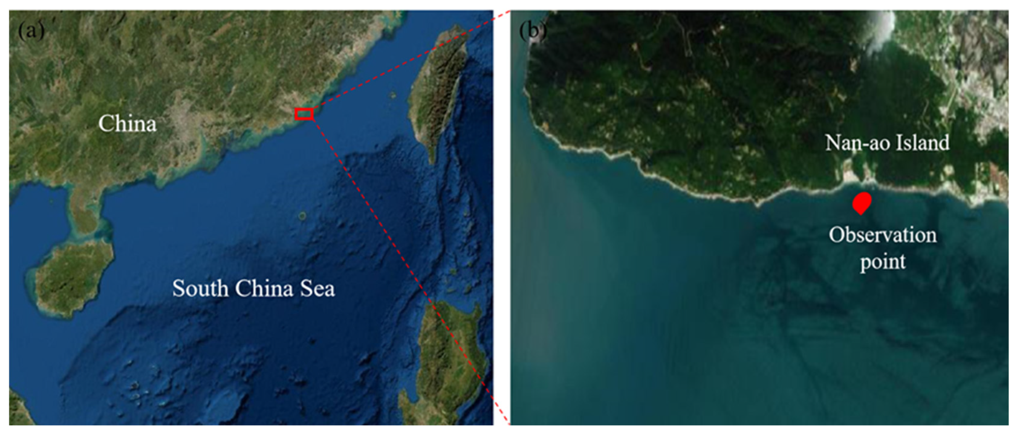
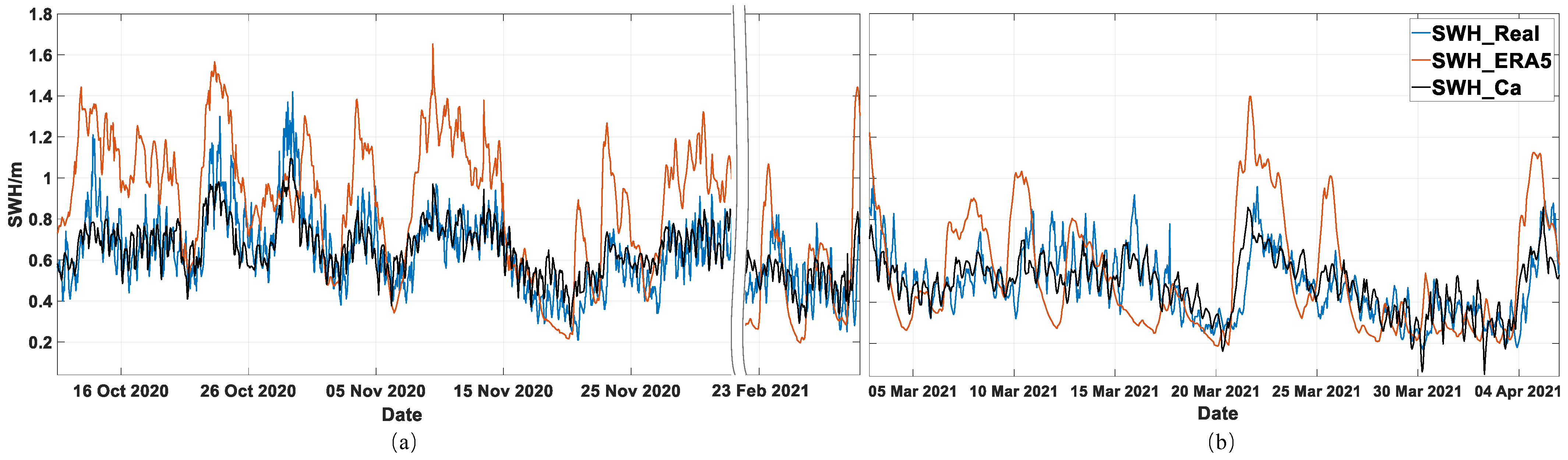
2.1. Data Used for Case Study

A case in the coastal area of the northeastern South China Sea is taken as an example to test the calibration algorithm proposed in this study. Nan-ao Island is a small island located in Shantou City, Guangdong Province, China. The location of the island and the observation site are shown in Figure 1. The field observation data used in this study came from the hydrological observation station deployed in the southern coastal waters. The station is about 300 m offshore and about 10 m deep. The wave, current, and tide levels were measured synchronically with the AWAC profiler manufactured by Nortek, Norway. Similar hydrological observation stations have been deployed in several inshore regions of the South China Sea [6,24]. The data from 11 October 2020 to 5 April 2021 are employed for the case study, and the observed SWH is defined as SWH_Real.
In this study, reanalysis data from the Fifth Generation Global Climate Reanalysis Dataset (ERA5) of the European Centre for Medium-Range Weather Forecasts (ECMWF) are used as numerical model output data for analysis. These data are generated by numerical prediction of climate elements using the WW3 model and assimilation with global sea area data. The data have been widely used in climate research, especially in wave prediction [25,26]. The ERA5 data in the same period and at the same location as the observation are employed. Variables including SWH, mean wave direction (MWD), and mean wave period (MWP) are obtained. To distinguish it from SWH_Real, the modeled SWH is defined as SWH_ERA5, and the calibrated SWH is defined as SWH_Ca.

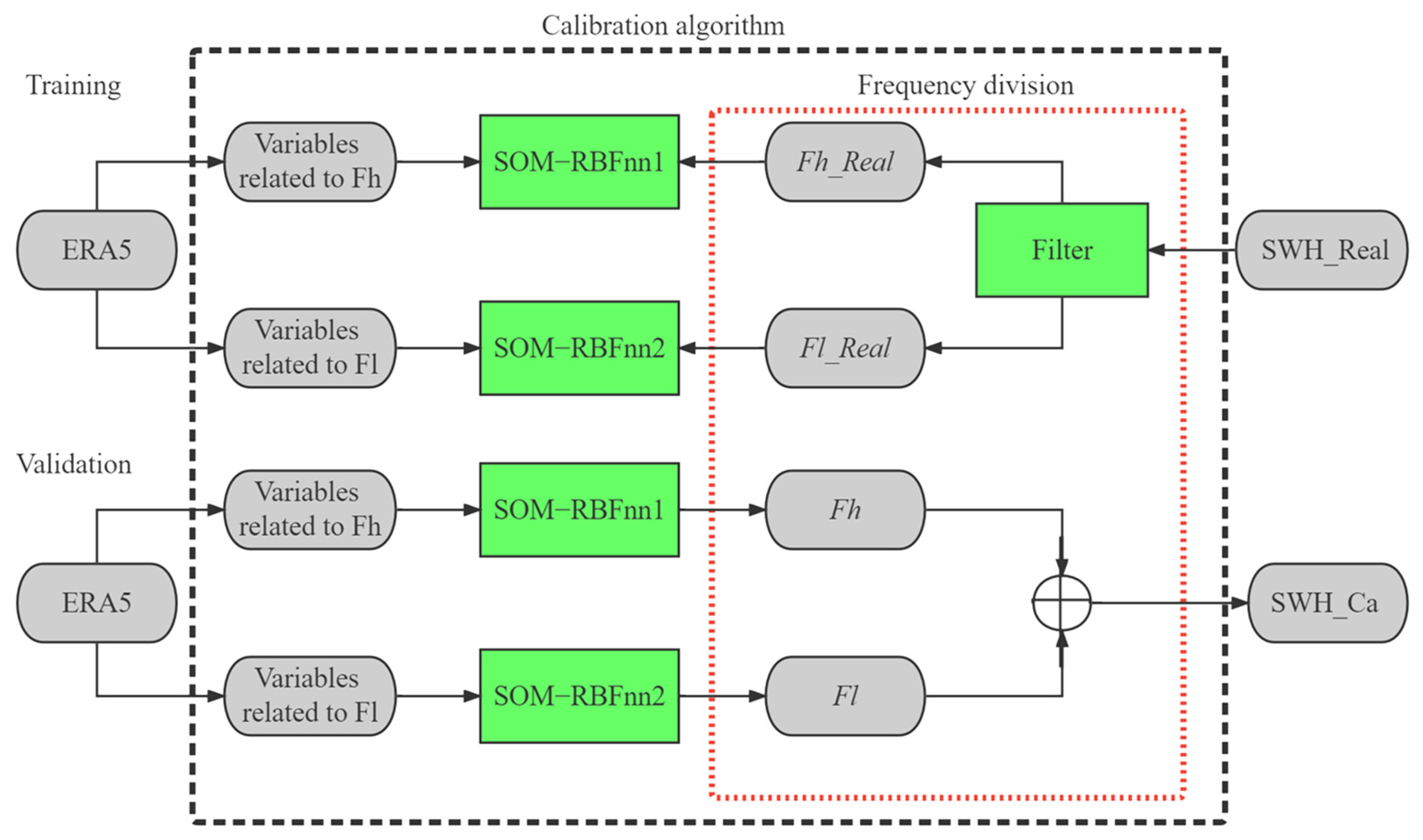
2.2. Calibration Algorithm for the Nearshore SWH

The algorithm constructed in this paper is used to realize the calibration for the model results, i.e., after inputting the modeled data at a certain time and place, the algorithm can derive the SWH_Ca, as close to the observation as possible. The calibration algorithm is constructed based on the SOM−RBFnn. The procedure of the algorithm is illustrated in Figure 2.

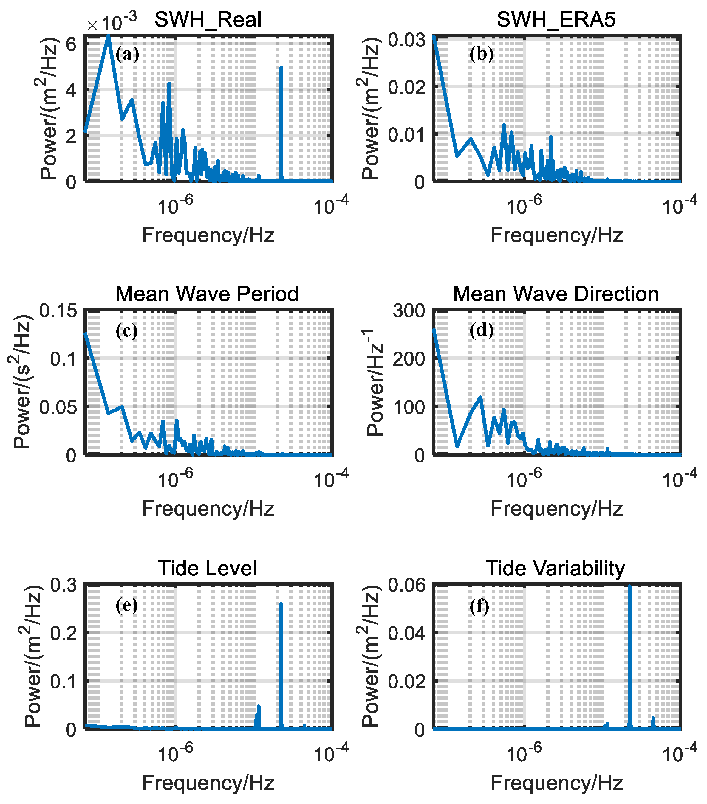
2.2.1. The Frequency Division

In the coastal waters, the currents forced by the tide have a direct effect on the wave [18,19,20,21,22,23]. When the wave encounters currents in the same direction, the wavelength increases, and the wave height decreases; when the wave encounters a reverse current, the wavelength decreases, and the wave height rises [21]. To consider this influence of the tidal current on the SWH, the high-frequency component of the SWH is separated and it is calibrated by the tidal factors. The fast Fourier transform (FFT) is performed to obtain the energy spectrum of the tidal and wave variables including SWH. For a variable X(k) with a data size of N, apply the discrete Fourier transform (DFT) and the formula is:
X ( k ) = n = 0 N 1 x ( n ) W N k n , k = 0 , 1 , 2 , , N 1
Due to the periodicity and symmetry of Wn, the FFT algorithm can decompose the N-point DFT transformation into the DFT at the N/2 point.
X ( k ) = X 1 ( k ) + W N k X 2 ( k ) , k = 0 , 1 , 2 , , N 2 1
X ( k + N 2 ) = X 1 ( k ) W N k X 2 ( k ) , k = 0 , 1 , 2 , , N 2 1
The upper formula is called the butterfly computation. According to this algorithm, the operation speed is increased by constant decomposition to two points, thus reducing the number of operations. In our algorithm, the purpose of using the Fourier transform is to separate the high-frequency variation of SWH affected by tide-driven current. Although in similar studies, the wavelet analysis method can also effectively separate the high-frequency variation [5,7], it focuses on the frequency at the local time domain, and the separation frequency will vary at different periods. However, because the frequency of tide is relatively fixed and does not change with time, it is more reasonable to use the Fourier transform to analyze SWH in the full-time domain.
Considering that the tide periods are mostly shorter than one day, we set 24 h as the frequency threshold to divide SWH_Real into the high-frequency part (Fh_Real) and the low-frequency part (Fl_Real):
SWH _ Real = F l _ R e a l + F h _ R e a l
In the training stage, Fh_Real was used to train the SOM−RBFnn1, and the Fl_Real was used to train the SOM−RBFnn2 (Figure 2). In the validation stage, the outputs of SOM−RBFnn1 (Fh) and SOM−RBFnn2 (Fl) are added to form SWH:
SWH _ Ca = F l + F h
We name this particular method as frequency division. In the algorithm, Fl is calibrated by SWH_ERA5, MWD, and MWP; Fh is calibrated by the variability of tide level (VT). This is because the tidal current in coastal areas is closely related to the change of tidal level (TL), and TL can be obtained by harmonic analysis, while the measurement of oceanic current is more complex.

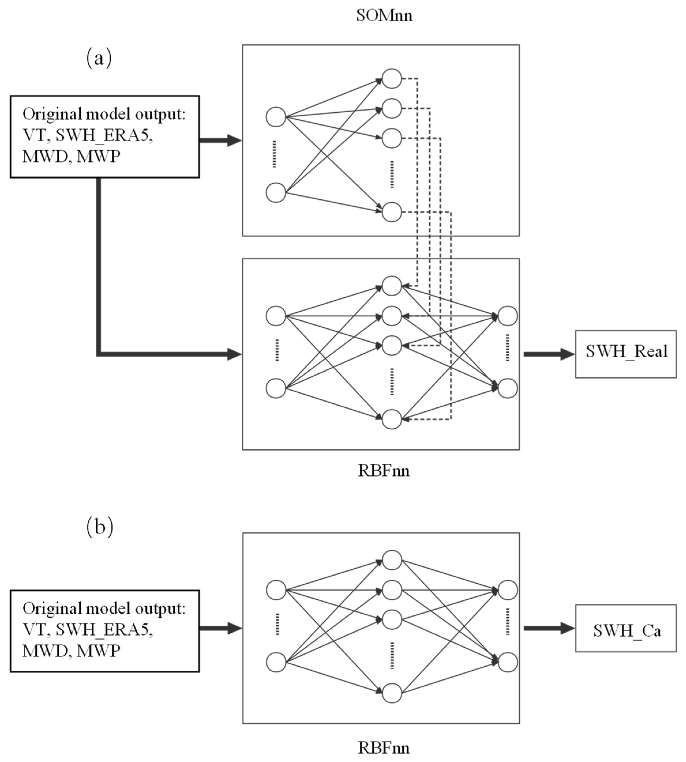
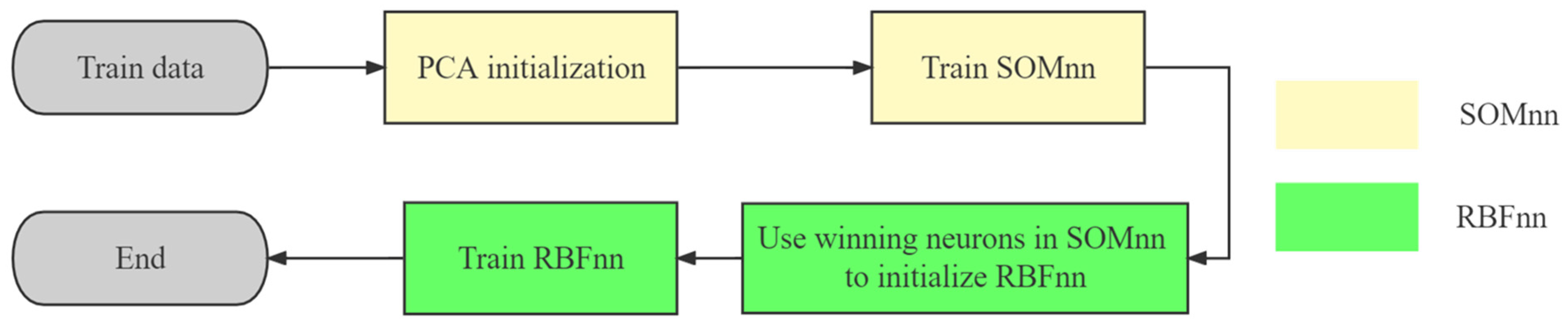
2.2.2. The SOM−RBFnn

The basic structure of the neural network and the connection between SOMnn and RBFnn is shown in Figure 3. RBFnn is a kind of forward neural network, which contains three layers: input layer, hidden layer, and output layer. The dimension of the center coordinates in the hidden layer neurons is consistent with the input space. During the training process, the RBFnn will first calculate the Euclidean distance between the sample and each center of the hidden layer, and input the distance into the radial basis function whose output is weighted and summed to form the RBFnn output. Weights connecting hidden neurons to output neurons can be determined by pseudo-inverse. The entire space should be covered by the receptive field of neurons in the hidden layer. Therefore, SOMnn is applied to cluster and determine center coordinates.
The SOMnn can cluster data by identifying the similarity between them without prior knowledge, through a competitive learning algorithm. First, the SOMnn is initialized by assigning node weight representing the center of the corresponding neuron, and its dimension is consistent with the input space. In one iteration, a sample randomly input to the SOMnn is compared with all the weights in the hidden layer (usually comparing the Euclidean distance between the sample and the weights), and the most similar node is selected as the best matching unit, which will drive itself and the nodes within a certain range closer to the sample. This entire process is reiterated until the specified number of iterations is achieved. After training, a node that becomes BMU at least once is recognized as an active node. Otherwise, it calls for an inactive node. The active nodes are used to optimize the RBFnn.
In our research, the SOM−RBFnn training process is performed in the following steps (see also Figure 4):
  • The node structure and scale of the SOMnn competition layer are specified. The rectangular competition layer structure is selected, and the number of nodes in the competition layer is determined to be 200 according to the data scale.
  • Competitive layer node weight initialization via principal component analysis.
  • Select xi as a sample, calculate the Euclidean distance between the sample and all nodes, and locate the node with the smallest distance from it,
    d j = arg min ( w t ( d j ) x i )
    where wt(dj) = wj,t representing the weight of node dj at the t-th iteration.
  • Update node weights by:
    w i , t + 1 = w i , t + η ( d j , d i ) × ( x i d i )
    where η(dj, di) is a neighborhood function, the size of which depends on the distance between node di and node dj, and it is used to characterize the influence of the BMU on its neighbors.
  • If the number of iterations t does not reach the set number of times tend, repeat steps 3 and 4; otherwise, define an active node-set A, which includes all active nodes when the iteration is completed, and proceed to the step.
  • Use the number and weight of SOMnn active nodes to initialize the hidden layer center ck = dk, dkA of the RBFnn, and the total number of hidden layer nodes N = crad(A).
  • The RBF hidden layer outputs hij = ϕ (||xicj||) correspond to the sample xi input. In this study, the radial basis function is selected as the Gaussian function:
    ϕ ( x i c j ) = exp ( x i c j 2 2 σ 2 )
  • Define the hidden layer output matrix H = [hij], and the weight matrix between the hidden layer to the output layer is WRBF = [w1RBF, w2RBF, …, wNRBF]T. The output of the RBFnn is Y = HWRBF. In the training phase, the output matrix Y is clamped, and the hidden layer output matrix H has been calculated through the above steps. Use the pseudo-inverse method to solve the weight matrix: WRBF = H−1Y.

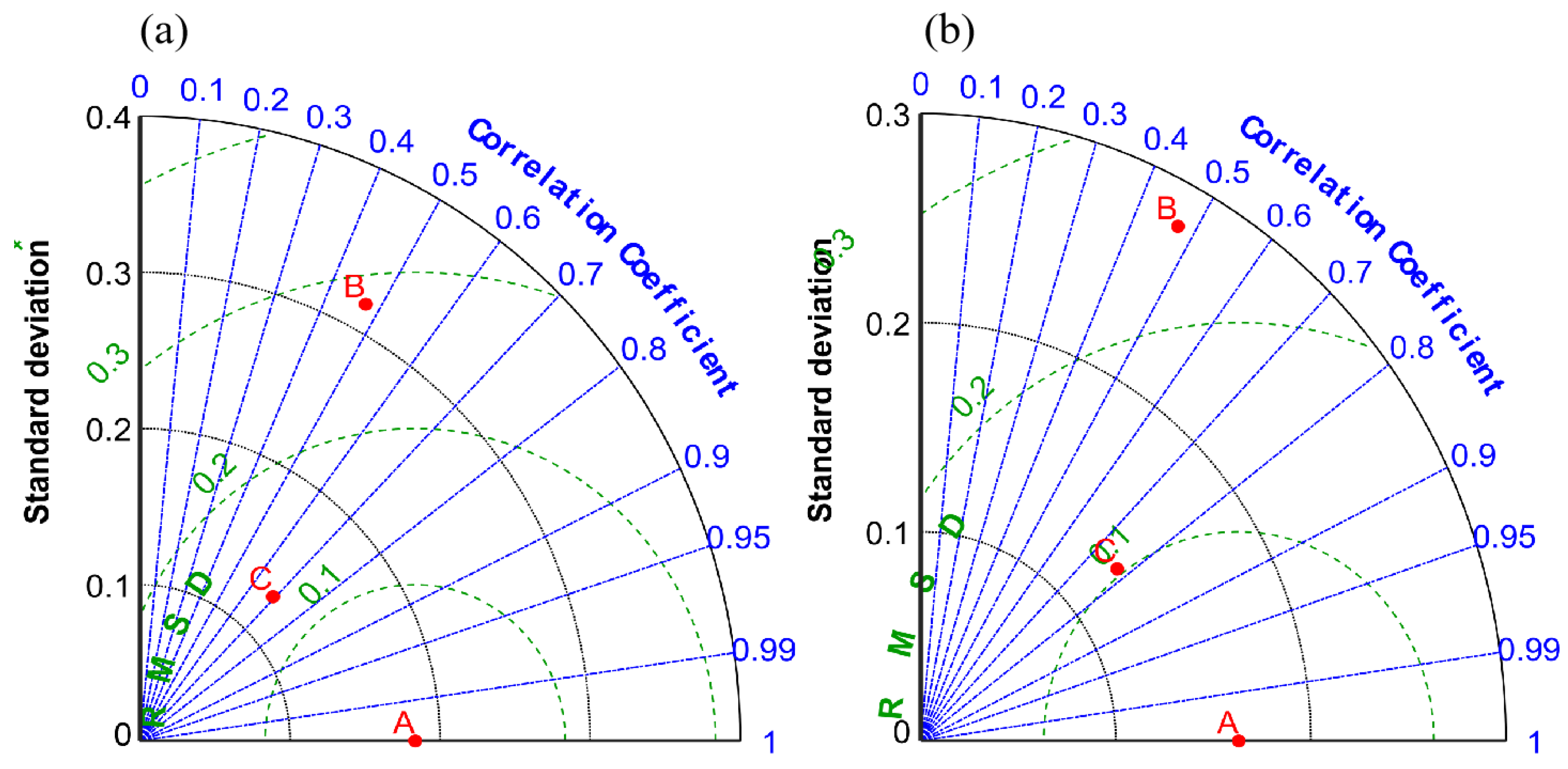
2.3. Performance Indicators

During the training process, the test set samples are input into the SOM−RBFnn, and the evaluation function is used to calculate the accuracy of the neural network. The root mean square error (RMSE), the mean absolute percent error (MAPE), and the scatter index (SI) are used to estimate the accuracy. They are calculated by:
RMSE = 1 n i = 1 n ( Y p r e d i c t i Y i ) 2
MAPE = 100 n i = 1 n | Y i Y p r e d i c t i Y i |
SI = i = 1 n ( Y i Y p r e d i c t i ) 2 n Y ¯ i
where Ypredicti is the modeled data, Yi is the observation data, and n is the number of samples. The closer the indexes are to 0, the better the algorithm is.
The in situ data and ERA5 model data were input into the calibration algorithm to test its performance in correcting SWH_ERA5. To further analyze the advantages of the algorithm, calibration experiments are carried out by comparing the SOM−RBFnn with the original RBFnn and Kmeans_RBFnn, and comparing the SOM−RBFnn with or without the frequency division.

3. Results

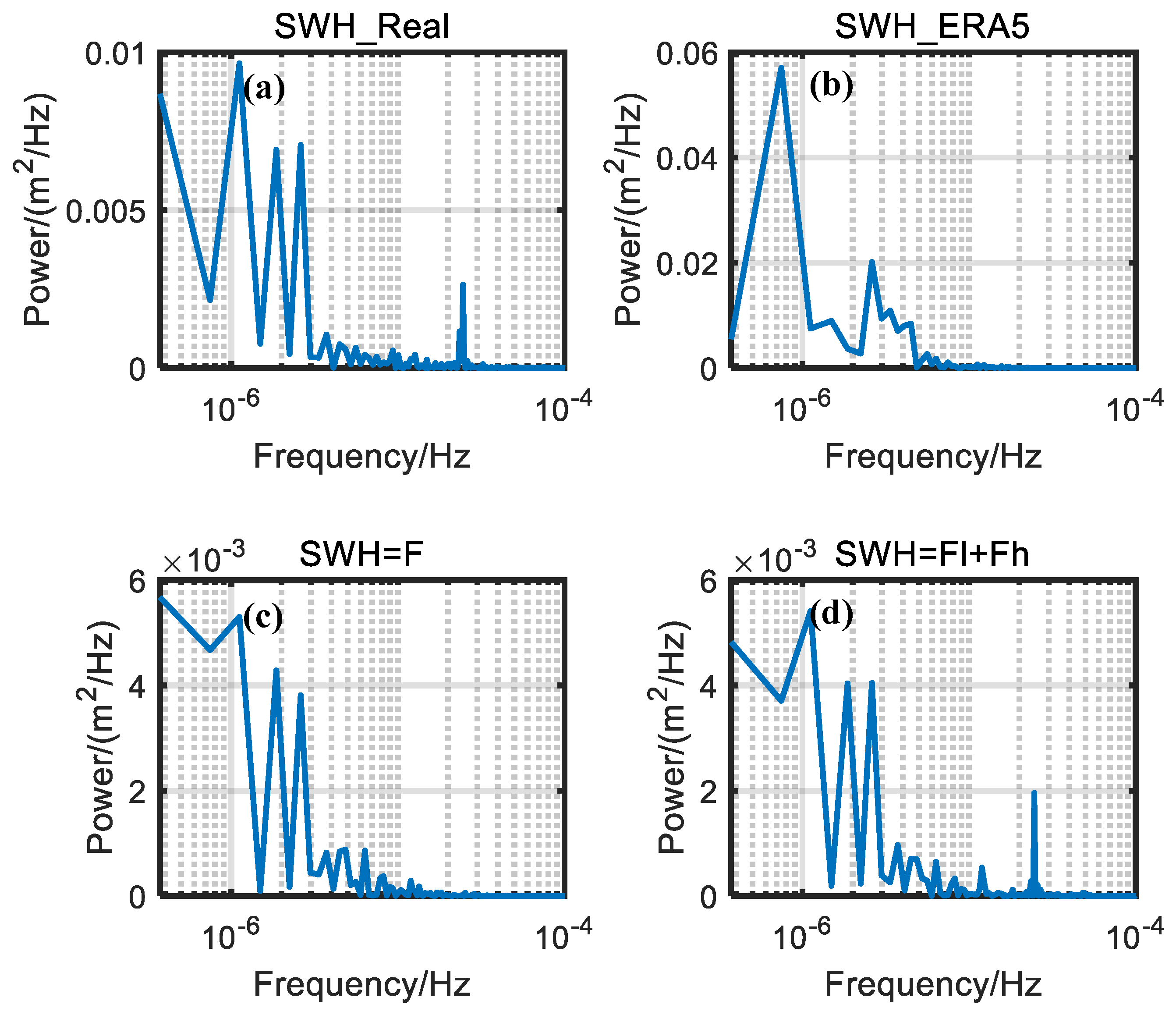
3.1. The Applicability of This Algorithm to the Study Case

To verify the frequency characteristics of the parameters (SWH_Real, SWH_ERA5, MWP, MWD, TL, and VT) relevant to the algorithm, a power spectrum analysis was performed (Figure 5). As shown in the figure, there occur two peak values in the spectrum of the SWH_Real corresponding to the low-frequency band and high-frequency band of 1.37 × 10⁻⁷ Hz and 2.24 × 10⁻⁵ Hz, respectively. The peak value of the high frequency is 0.005 m2/Hz and the corresponding period is 12.4 h, which is consistent with the period of the VT. In addition, SWH_ERA5, MWP, and MWD are all concentrated in the low-frequency band and the variation of high-frequency factors such as the nearshore tide is not taken into account. Thus, it is difficult to realize the effective simulation or prediction of wave parameters without tidal information.
The energy density of TL and VT are consistent with tidal characteristics, concentrated in multiple high-frequency bands with corresponding cycles of 24h, 12h, and 6h, respectively. Among them, the energy in the 12 h frequency band is the highest, which is consistent with the high-frequency energy peak value of SWH. Considering that tidal variation is mainly diurnal, 24 h frequency is taken as the threshold and then Fh_Real can be separated from Fl_Real.
Correlation analysis and significance tests were conducted on the above parameters. Pearson’s correlation coefficients (R) are shown in Table 1. Based on the analysis results, Fl_Real is significantly relative to SWH_ERA5, MWP, MWD, TL, and VT, with much higher R values versus SWH_ERA5, MWP, and MWD. On the other side, Fh_Real is significantly relative to MWP, TL, and VT, with much higher R values versus VT. These results further confirm the applicability of the frequency division method of our algorithm that Fl is calibrated by SWH_ERA5, MWD, and MWP, while Fh is by VT (see Section 2.2).

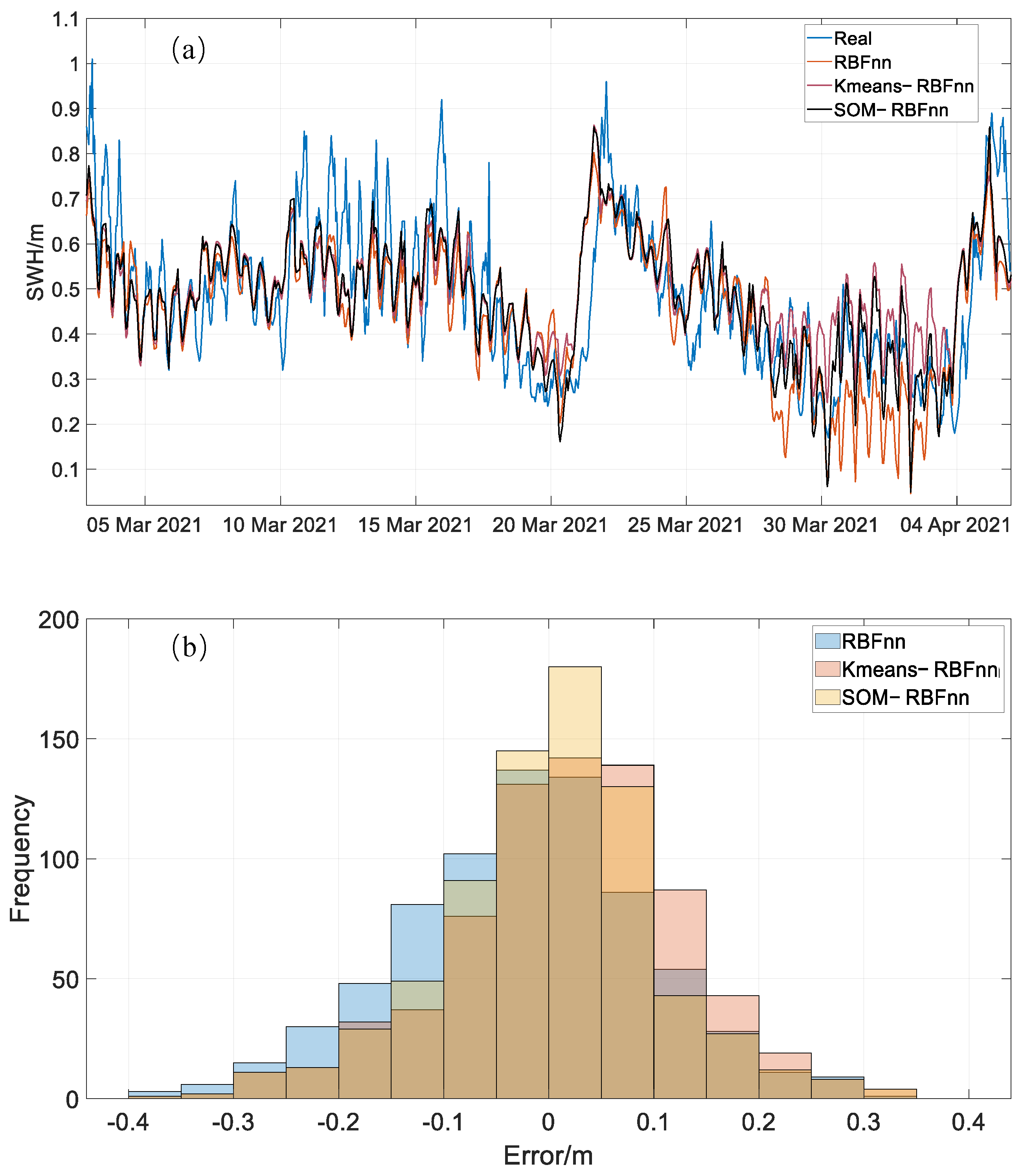
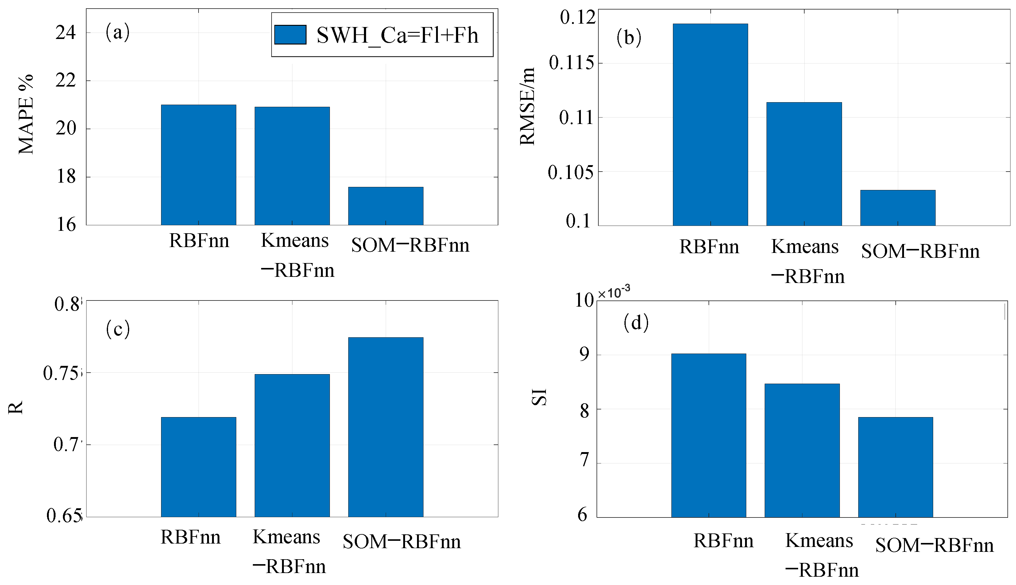
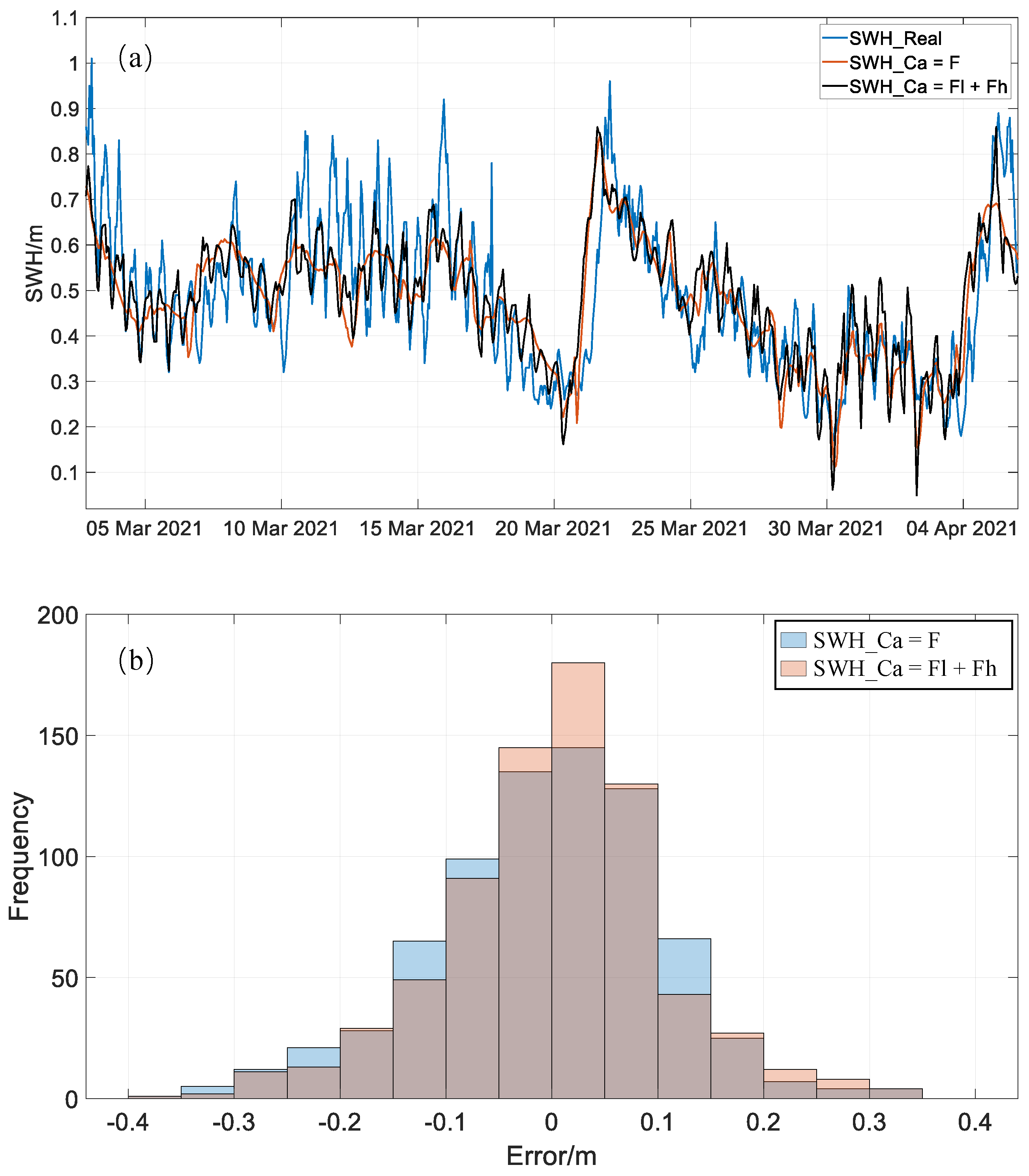
3.2. Calibration Results of the Case Study

The algorithm proposed in the study is used to calibrate the SWH_ERA5 in the case of the coastal area of Nan-ao Island (Figure 1). The calibration results in time series and Taylor diagrams are presented in Figure 6 and Figure 7, respectively. The results mainly demonstrate that the accuracy of the SWH_Ca is greatly improved. For example, RMSE reduces from 0.252 m to 0.103 m, MAPE reduces from 41% to 17.6%, and R increases from 0.472 to 0.774. In Figure 6, although the general variation of SWH_Real can be modeled, the deviation of the SWH_ERA5 is prominent, and it is more evident for some extreme values. After the calibration by the algorithm, both the general variation and the high-frequency changes of SWH_Ca are closer to the observation values than SWH_ERA5. Taylor diagrams further confirm the effect of the calibration algorithm (Figure 7). In the figure, the statistical indicators of the calibrated results (Point C) are closer to the reference point (Point A). The above results illustrate the good performance of the calibration algorithm.

4. Discussion

4.1. Advantages of SOM−RBFnn

The calibration algorithm proposed in this study is based on the SOM−RBFnn. To examine its relative advantages compared to similar artificial neural networks, e.g., the original RBFnn that randomly determines initial node coordinates in the hidden layer and the RBFnn optimized based on the Kmeans algorithm (Kmeans_RBFnn), a control experiment was performed. In the experiment, the results of SOM−RBFnn in the above sections are regarded as a reference. By comparison, the original RBFnn and Kmeans_RBFnn, respectively, are used to replace the SOM−RBFnn in our algorithm, and the calibration for the case study is repeated with all other settings remaining.
The results of the control experiment show that all three neural networks can improve the model results to match the observation data in the general trend, but there are specific differences in some important details (Figure 8). The results with SOM−RBFnn appear to better improve the errors of modeled SWH, compared to the other two neural networks. For example, during the simulation period, the SOM−RBFnn error diagram is more concentrated near zero than the other two neural networks (Figure 8b). Moreover, from the perspective of statistical indicators, compared with the other two neural networks, the calculation results of SOM−RBFnn are impressively lower in MAPE, RMSE, and SI, and higher in the R-value (Figure 9).
The reason for SOM−RBFnn having the best performance is because SOMnn, compared with the other two clustering methods, can better perform unsupervised clustering, find the center point of the sample, and more effectively specify the coordinates of neurons in the middle layer of RBFnn [15,16,17]. Therefore, the trained SOMnn will perform unsupervised clustering on the input and assign the number and coordinates of the RBFnn hidden layer nodes, which can optimize the hidden layer neurons of RBF, reduce training time, and improve the model performance.
In the studies of intelligent prediction or calibration of SWH, different types of artificial neural networks were constructed according to their specific requirements. For the model of predicting SWH based on past and current information, neural networks with memory functions, such as gated recurrent unit networks [8] and long short-term memory networks [9], were usually used. For models that focus on high-frequency variation of SWH, wavelet analysis is usually combined with their neural networks [5,7]. Similarly, in this study, SOM−RBFnn is used to better reflect the clustering characteristics among SWH and relevant variables such as MWP, MWD, and VT. As a result, the constructed algorithm can well correct the SWH output from the ERA5 model (Figure 8 and Figure 9).

4.2. Efficacy of Frequency Division Method

To examine the efficacy of the frequency division method in our calibration algorithm, another control experiment was performed. In the experiment, SWH_Ca was no longer processed by Equation (5); instead, it was directly calibrated by the input parameters of SWH_ERA5, MWP, and MWD (i. e., SWH_Ca = F), and the calibration for the case study was repeated with all other settings remaining.
The numerical experimental results show that the calibration effect with the frequency division method is much better (Figure 10). In Figure 10a, the results applying SWH_Ca = Fl + Fh are closer to the observational data, while the results with SWH_Ca = F cannot reflect the extreme values of the real wave height. In addition, the error distribution illustrated in Figure 10b shows that the errors calibrated by SWH_Ca = Fl + Fh tend more to concentrate around zero, which indicates the results have more centralized error distributions.
Because wave height is mainly impacted by the tidal current in the nearshore areas [18,19,20,21], the frequency division method should be applied to calibrate the high-frequency component of SWH separately. The importance of the frequency division method can be further illustrated by the power spectrum of the two calibration results in Figure 11. The spectrum of SWH_Real has a high-frequency peak corresponding to a period of approximately 12 h (Figure 11a), which is decided by the factor of tidal currents. For example, when the daily changing current direction and the wave direction are opposite (or the same), the wave height will increase (or decrease) [21]. However, SWH_ERA5 does not have this high-frequency peak (Figure 11b). Thus, if the factor of tidal currents is not taken into account, the calibration results would not be able to characterize the high-frequency features (Figure 11c). In our algorithm, by dividing the data into low-frequency and high-frequency components, and choosing relevant variables to respectively calibrate them, the results will perform a better simulation of the coastal SWH with a reasonable high-frequency variation characteristic (Figure 11d).
Previous studies on SWH prediction have also added the special treatment of high-frequency variation of SWH to their models. In the models, the high-frequency parts are mainly separated by wavelet analysis [5,7]. In contrast, the biggest difference in our algorithm is that the high-frequency variation part is separated by the Fourier transform (i. e., Equations (1)–(5)). This treatment is undertaken because the high-frequency variation of nearshore waves concerned in this study is mainly determined by tidal-driven currents [18,19,20,21]. The frequency of tides is relatively fixed and does not change with time. Thus, it is more reasonable to use the Fourier transform to analyze the whole scale of SWH than the wavelet decomposition that integrates the local changes of time and frequency. The results of the experiment also verify the effectiveness of this treatment (Figure 10 and Figure 11).

5. Conclusions

It is difficult for common wave numerical models to effectively depict the complex coastline boundary and relative dynamic processes in nearshore areas, probably because of the limitations of spatial resolutions and parametric schemes. This can easily lead to an apparent deviation in the simulation and prediction of wave parameters, such as significant wave height (SWH). To solve this problem, we propose an intelligent algorithm for the calibration of the modeled SWH in nearshore areas. The core of the algorithm is based on the self-organizing map–radial basis function neural network (SOM−RBFnn). In addition, the algorithm uses a frequency division method, which separates the relatively high-frequency variation within 24 h of SWH and calibrates it independently. Based on the in situ observations and the corresponding model data output by ERA5 at a typical coastal site in the northeastern South China Sea, the feasibility of the algorithm is verified by the increase in the correlation coefficient from 0.472 to 0.774, as well as the decreases in the root mean square error from 0.252 m to 0.103 m and the mean relative error from 41% to 17.6%. Control experiments are performed to prove the advantages of SOM−RBFnn compared to other similar artificial neural networks. Moreover, the experiment further confirms that the frequency division method can better simulate the high-frequency variations of the coastal waves. Therefore, the combination of SOM−RBFnn and the frequency division method appears to have a good performance in calibrating SWH in our algorithm. This algorithm can be useful to correct the model-predicted SWH for marine hydrological information support applications and produce high-quality hydrodynamics data for further oceanography studies.

Author Contributions

Conceptualization, H.H. and J.L. (Junmin Li); methodology, H.H.; software, H.H. and Z.H.; validation, J.L. (Junmin Li), and B.L.; formal analysis, Z.H. and Y.L.; investigation, L.S., J.L. (Junliang Liu) and W.C.; resources, L.S., J.L. (Junliang Liu) and W.C.; data curation, B.L. and W.C.; writing—original draft preparation, H.H., Z.H. and Y.L.; writing—review and editing, J.L. (Junmin Li); visualization, Z.H. and Y.L.; supervision, H.H. and J.L. (Junmin Li); project administration, H.H., J.L. (Junmin Li); funding acquisition, J.L. (Junmin Li). All authors have read and agreed to the published version of the manuscript.

Funding

This study is supported by the Hainan Provincial Natural Science Foundation of China (422MS160), the Science and Technology Plan Projects of Guangdong Province (2021B1212050025), the Key Special Project for Introduced Talents Team of Southern Marine Science and Engineering Guangdong Laboratory (Guangzhou) (GML2019ZD0303), CAS Key Laboratory of Science and Technology on Operational Oceanography (OOST2021-02), and 2021 Innovation Training Programs for Undergraduates, CAS.

Data Availability Statement

The data are available from the corresponding authors by request.

Acknowledgments

The deployments of the hydrological monitoring platforms were supported by Shantou Station and Nan-ao Station, Shanwei Marine Environment Monitoring Center, State Oceanic Administration. The analysis in this study is supported by the High-Performance Computing Division at the South China Sea Institute of Oceanology.

Conflicts of Interest

The authors declare no conflict of interest.

References

  1. Adytia, D.; Saepudin, D.; Pudjaprasetya, S.R.; Husrin, S.; Sopaheluwakan, A. A deep learning approach for wave forecasting based on a spatially correlated wind feature, with a case study in the Java Sea, Indonesia. Fluids 2022, 7, 39. [Google Scholar] [CrossRef]
  2. Brus, S.R.; Wolfram, P.J.; Van Roekel, L.P.; Meixner, J.D. Unstructured global to coastal wave modeling for the Energy Exascale Earth System Model using WAVEWATCH III version 6.07. Geosci. Model. Dev. 2021, 14, 2917–2938. [Google Scholar] [CrossRef]
  3. Inghilesi, R.; Orasi, A.; Catini, F. The ISPRA Mediterranean coastal wave forecasting system: Evaluation and perspectives. J. Oper. Oceanogr. 2016, 9, s89–s98. [Google Scholar] [CrossRef]
  4. Deo, M.C.; Jha, A.; Chaphekar, A.S.; Ravikant, K. Neural networks for wave forecasting. Ocean Eng. 2001, 28, 889–898. [Google Scholar] [CrossRef]
  5. Deshmukh, A.N.; Deo, M.C.; Bhaskaran, P.K.; Nair, T.M.B.; Sandhya, K.G. Neural-network-based data assimilation to improve numerical ocean wave forecast. IEEE J. Oceanic 2016, 41, 944–953. [Google Scholar] [CrossRef]
  6. Li, B.; Li, J.; Li, Y.; Zhang, Z.; Shi, P.; Liu, J.; Chen, W. Application of artificial neural network to numerical wave simulation in the coastal region of island. J. Xiamen Univ. (Nat. Sci.) 2020, 59, 420–427. (In Chinese) [Google Scholar] [CrossRef]
  7. Chen, D.; Liu, F.; Zhang, Z.; Lu, X.; Li, Z. Significant wave height prediction based on wavelet graph neural network. In Proceedings of the 2021 IEEE 4th International Conference on Big Data and Artificial Intelligence (BDAI), Qingdao, China, 2–4 July 2021; pp. 80–85. [Google Scholar] [CrossRef]
  8. Wang, J.; Wang, Y.; Yang, J. Forecasting of significant wave height based on gated recurrent unit network in the Taiwan Strait and its adjacent waters. Water 2021, 13, 86. [Google Scholar] [CrossRef]
  9. Zhou, S.; Bethel, B.J.; Sun, W.; Zhao, Y.; Xie, W.; Dong, C. Improving significant wave height forecasts using a joint empirical mode decomposition–long short-term memory network. J. Mar. Sci. Eng. 2021, 9, 744. [Google Scholar] [CrossRef]
  10. Namigtle-Jiménez, A.; Escobar-Jiménez, R.F.; Gómez-Aguilar, J.F.; García-Beltrán, C.D.; Téllez-Anguiano, A.C. Online ANN-based fault diagnosis implementation using an FPGA: Application in the EFI system of a vehicle. ISA Trans. 2020, 100, 358–372. [Google Scholar] [CrossRef]
  11. Carbot-Rojas, D.A.; Escobar-Jiménez, R.F.; Gómez-Aguilar, J.F.; García-Morales, J.; Téllez-Anguiano, A.C. Modelling and control of the spark timing of an internal combustion engine based on an ANN. Combust. Theory Model. 2020, 24, 510–529. [Google Scholar] [CrossRef]
  12. Qasem, S.N.; Shamsuddin, S.M.; Zain, A.M. Multi-objective hybrid evolutionary algorithms for radial basis function neural network design. Knowl. Based Syst. 2012, 27, 475–497. [Google Scholar] [CrossRef]
  13. Kamel, A.H.; Afan, H.A.; Sherif, M.; Ahmed, A.N.; El-Shafie, A. RBFNN versus GRNN modeling approach for sub-surface evaporation rate prediction in arid region. Sustain. Comput. Inform. Syst. 2021, 30, 100514. [Google Scholar] [CrossRef]
  14. Guo, X.-G.; Tian, M.-E.; Li, Q.; Ahn, C.K.; Yang, Y.-H. Multiple-fault diagnosis for spacecraft attitude control systems using RBFNN-based observers. Aerosp. Sci. Technol. 2020, 106, 106195. [Google Scholar] [CrossRef]
  15. Lv, Z.; Xiao, F.; Wu, Z.; Liu, Z.; Wang, Y. Hand gestures recognition from surface electromyogram signal based on self-organizing mapping and radial basis function network. Biomed. Signal. Proces. 2021, 68, 102629. [Google Scholar] [CrossRef]
  16. Fu, H.; Liu, T.; Zhang, S.; Zhao, D.; Ding, G. Gas emission quantity dynamic prediction model of coal mine based on SOM-RBF algorithm. Chin. J. Sens. Actuators 2015, 28, 1255–1261. (In Chinese) [Google Scholar] [CrossRef]
  17. Rumbell, T.; Denham, S.L.; Wennekers, T. A spiking self-organizing map combining STDP, oscillations, and continuous learning. IEEE Trans. Neural Netw. Learn. 2014, 25, 894–907. [Google Scholar] [CrossRef] [Green Version]
  18. Song, H.; Kuang, C.; Gu, J.; Zou, Q.; Liang, H.; Sun, X.; Ma, Z. Nonlinear tide-surge-wave interaction at a shallow coast with large scale sequential harbor constructions. Estuar. Coast. Shelf Sci. 2020, 233, 106543. [Google Scholar] [CrossRef]
  19. Uchiyama, Y.; McWilliams, J.C.; Shchepetkin, A.F. Wave–current interaction in an oceanic circulation model with a vortex-force formalism: Application to the surf zone. Ocean Model. 2010, 34, 16–35. [Google Scholar] [CrossRef]
  20. Liu, W.-C.; Huang, W.-C. Investigating typhoon-induced storm surge and waves in the coast of Taiwan using an integrally-coupled tide-surge-wave model. Ocean Eng. 2020, 212, 107571. [Google Scholar] [CrossRef]
  21. Qi, W.-G.; Li, C.-F.; Jeng, D.-S.; Gao, F.-P.; Liang, Z. Combined wave-current induced excess pore-pressure in a sandy seabed: Flume observations and comparisons with theoretical models. Coast. Eng. 2019, 147, 89–98. [Google Scholar] [CrossRef] [Green Version]
  22. Yang, Q.; Ou, J.; Li, Y.; Huang, N. Effects of tidal-current and tidal-level changes on waves in the Yangtze River estuary. J. Trop. Oceanogr. 2015, 34, 19–26. (In Chinese) [Google Scholar] [CrossRef]
  23. Wu, Z.; Jing, C.; Deng, B.; Cao, Y. SWAN-ROMS coupling model and its application in idealized tidal inlets. J. Harbin Eng. Univ. 2019, 40, 1420–1426. [Google Scholar] [CrossRef]
  24. Li, B.; Chen, W.; Liu, J.; Li, J.; Wang, S.; Xing, H. Construction and application of nearshore hydrodynamic monitoring system for uninhabited islands. J. Coast. Res. 2020, 99, 131–136. [Google Scholar] [CrossRef]
  25. Wang, J.; Liu, J.; Wang, Y.; Liao, Z.; Sun, P. Spatiotemporal variations and extreme value analysis of significant wave height in the South China Sea based on 71-year long ERA5 wave reanalysis. Appl. Ocean Res. 2021, 113, 102750. [Google Scholar] [CrossRef]
  26. Li, B.; Chen, W.; Li, J.; Liu, J.; Shi, P.; Xing, H. Wave energy assessment based on reanalysis data calibrated by buoy observations in the southern South China Sea. Energy Rep. 2022, 8, 5067–5079. [Google Scholar] [CrossRef]
Figure 1. Location of the observation station for the case study. (a) shows the relative location of Nao-ao Island in the northern South China Sea, and (b) shows the specific location of the station to the south of Nan-ao Island.
Jmse 10 00706 g001
Figure 2. The procedure of the calibration algorithm with the frequency division method and the self-organizing map–radial basis function neural network (SOM−RBFnn).
Jmse 10 00706 g002
Figure 3. Schematic diagram of the SOM−RBFnn in the (a) training and (b) validation stages. SWH_ERA5, SWH_Real, and SWH_Ca represent the SWH originally output from the ERA5 model, the observed SWH, and the calibrated SWH, respectively. VT, MWD, and MWP are the variability of tide level, mean wave direction, and mean wave period, respectively.
Jmse 10 00706 g003
Figure 4. Flowchart of the training process of SOM−RBFnn.
Jmse 10 00706 g004
Figure 5. Diagrams of the power spectrums of (a) observational significant wave height (SWH_Real), (b) ERA5 significant wave height (SWH_ERA5), (c) ERA5 mean wave period (MWP), (d) ERA5 mean wave direction (MWD), (e) tidal level (TL), and (f) tidal variability (VT).
Jmse 10 00706 g005
Figure 6. Comparison of SWH_Real, SWH_ERA5, and SWH_Ca in time series of the (a) training and (b) validation stages.
Jmse 10 00706 g006
Figure 7. Taylor diagrams of the SWH_Real (point A), SWH_ERA5 (point B), and SWH_Ca (point C) in the (a) training dataset and (b) validation stages.
Jmse 10 00706 g007
Figure 8. Performance comparison among RBFnn, Kmeans−RBFnn, and SOM−RBFnn in (a) time series and (b) error histogram.
Jmse 10 00706 g008
Figure 9. The performance comparison of three neural networks (RBFnn, Kmeans−RBFnn, and SOM−RBFnn). (a) MAPE; (b) RMSE; (c) R; (d) SI.
Jmse 10 00706 g009
Figure 10. Comparison between the calculation results of whether to apply the frequency division method in (a) time series and (b) error histogram.
Jmse 10 00706 g010
Figure 11. The power spectrum of (a) SWH_Real, (b) SWH_ERA5, and the calibration results where (c) SWH_Ca is treated as a whole variable (SWH_Ca = F) and (d) SWH_Ca is divided into high− and low−frequency parts (SWH_Ca = Fl + Fh).
Jmse 10 00706 g011
Table 1. Correlation analysis results.
SWH_ERA5MWPMWDTLVT
Fl_Real0.566 *0.700 *−0.337 *0.223 *0.0731 *
Fh_Real0.02990.0529 *−0.01270.287 *0.598 *
SWH_Real0.523 *0.653 *−0.310 *0.298 *0.267 *
* means p < 0.001.
Publisher’s Note: MDPI stays neutral with regard to jurisdictional claims in published maps and institutional affiliations.

