Coordinated Formation Control of Discrete-Time Autonomous Underwater Vehicles under Alterable Communication Topology with Time-Varying Delay

Abstract

This paper is concerned with the coordinated formation control problem of multiple autonomous underwater vehicles (AUVs) under alterable communication topology and time-varying delay in discrete time domain. Firstly, the multi-AUV system is divided into one leader and multiple followers, and the communication topology is divided into two parts. The coupled nonlinear AUV model is linearized into a second-order integral model using state feedback. Secondly, two types of coordinated controllers in discrete time are proposed: the controller for multi-AUV system without delay, the controller for multi-AUV system with time-varying delay. Then, the formation control issue for multiple AUVs with alterable topology is treated as the asymptotic stability of an error system. The stability analysis of the error system consisting of the state errors between each follower and the leader is performed, to obtain some novel sufficient conditions for achieving the formation control objective. Finally, some simulation results are presented to demonstrate the effectiveness of the theoretical results, and the comparisons describe the effects of communication topology and delay on the performance of the control system.

1. Introduction

With the exploration and utilization of marine resources, the coordinated control of autonomous underwater vehicles (AUVs) has been paid more and more attention [1,2]. Compared with a single AUV, multi-AUV formation equipped with more sensors can complete more complex and larger ocean missions through information exchange between AUVs [3]. However, affected by the complicated sea conditions or vehicle accidents, the transmission of information between AUVs may be interrupted, resulting in the inability to communicate information within the multi-AUV system, so coordination of the system should be guaranteed in the case of emergencies [4].

In recent years, many scholars have made significant progress in the motion control of AUV monomers. In a complex operating environment, some tracking or searching tasks can be accomplished through such control methods as adaptive control [5,6], robust control [7,8], and fuzzy control [9,10], etc. In Ref. [5], an adaptive control strategy is developed to handle the region tracking control problem of AUVs based on prescribed performance theory and backstepping mechanism. A robust model predictive control is presented for underactuated AUV subject to multiple state constraints and external uncertainties in [7]. In consideration of the uncertain parameters of the AUV model, one adaptive fuzzy control law which is based on Gaussian function is formulated to ensure the stability of the tracking control system in [10]. These approaches can accomplish excellent motion control tasks for a single AUV, but coordinated control techniques for multiple AUVs also require intense development. To solve the problem of formation control of the AUV, some traditional nonlinear control methods have been used in the previous literature. Cui proposed a backstepping controller for leader-following formation control of underactuated AUV in [11], the controller can control the formation members to track the reference trajectory according to the position of the leader and the desired formation without velocity. In [12], Qi designed an adaptive distributed controller for AUV, which can finally make each AUV form the desired formation on the preset path. Ref. [13] solved the formation–containment control problem of AUVs by employing a two-layer control framework consisting of the leader layer and the follower layer. To enable multiple AUVs suffering from external perturbations to track the reference trajectory and maintain appropriate formation, Ref. [14] proposed a distributed Lyapunov-based model predictive controller. The aforementioned literatures primarily focus on the control algorithms for formation systems, they do not concern the influence of communication between AUVs on the control system.

Meanwhile, consensus theory is one of the most momentous approaches of the coordinated formation control of a multi-agent system. In multi-agent system, the consensus is defined as that all agents maintain the common state in positions, velocities and attitudes [15]. More development process of the consensus algorithm is described in [16,17]. The early consensus algorithm was applied to the first-order multi-agent system under the condition of random communication topology and communication disturbance [18,19], which also laid the foundation for the consensus research of second-order multi-agent [20,21,22]. Illuminated by the coordinated control of multi-UAV [23,24,25], some consensus algorithms have been applied to multi-AUV system [26,27]. In [28], Yan proposes a control protocol with additional functions to solve the formation control problem when considering environmental disturbances. Ref. [29] addresses a leader-following consensus control protocol for multi-AUV recovery system with time-varying delay. The AUV formation trajectory tracking control problem in a class of weak communication environment is investigated in [30]. Different from the communication on the land, the communication of the multi-AUV system in the ocean will be affected by various factors, which include the time delay due to the slow transmission rate of sound waves and the information transmitter or receiver of some vehicles cannot work properly. Moreover, some coordinated control provided by using a consensus algorithm may ignore the nonlinear and coupling parameters in the vehicle dynamics. Therefore, accurate models suitable for consensus algorithms and complex communication conditions are serious challenges in the application of combining of consensus and coordinated control problem of multi-AUV formation.

Based on the above discussion, the coordinated formation control issue of multi-AUV system with alterable communication topology and time-varying delay in discrete time domain will be discussed in this paper. In order to ensure the accuracy of AUVs control system and simplify the nonlinear coordinated control problem, the state feedback technique is employed to derive the discrete-time AUV model. The main contributions are as follows.

(1)

Depending on the presence or absence of communication delay, two feasible coordinated controllers are designed to guarantee that multiple AUVs can achieve formation in the discrete time domain.

(2)

The error system between the leader and the followers is constructed and new sufficient conditions to keep it asymptotically stable are derived. Based on these conditions, practicable controller gains can be deduced, as well as constraints on the alterable communication topology.

(3)

In order to validate the feasibility of the main theoretical results, two-dimensional and three-dimensional multiple AUVs simulations are carried out, respectively. The results are compared to show the power of different communication conditions on the control system.

2. Preliminaries

2.1. Notations

In this paper, ⊗ represents the Kronecker product, and $det(\cdot )$ is the determinant of a matrix. $\mathbb{R}$ indicates the real number set, ${\mathbb{R}}^m$ denotes the $m\times 1$ column vector, and ${\mathbb{R}}^{n\times m}$ is $n\times m$ matrix. $I_n$ represents the identity matrix with n dimensions, $A^T$ is the transpose of matrix A, $∥\cdot ∥$ stands for the Euclidean norm, and $\left|\cdot \right|$ denotes the modulus of complex number.

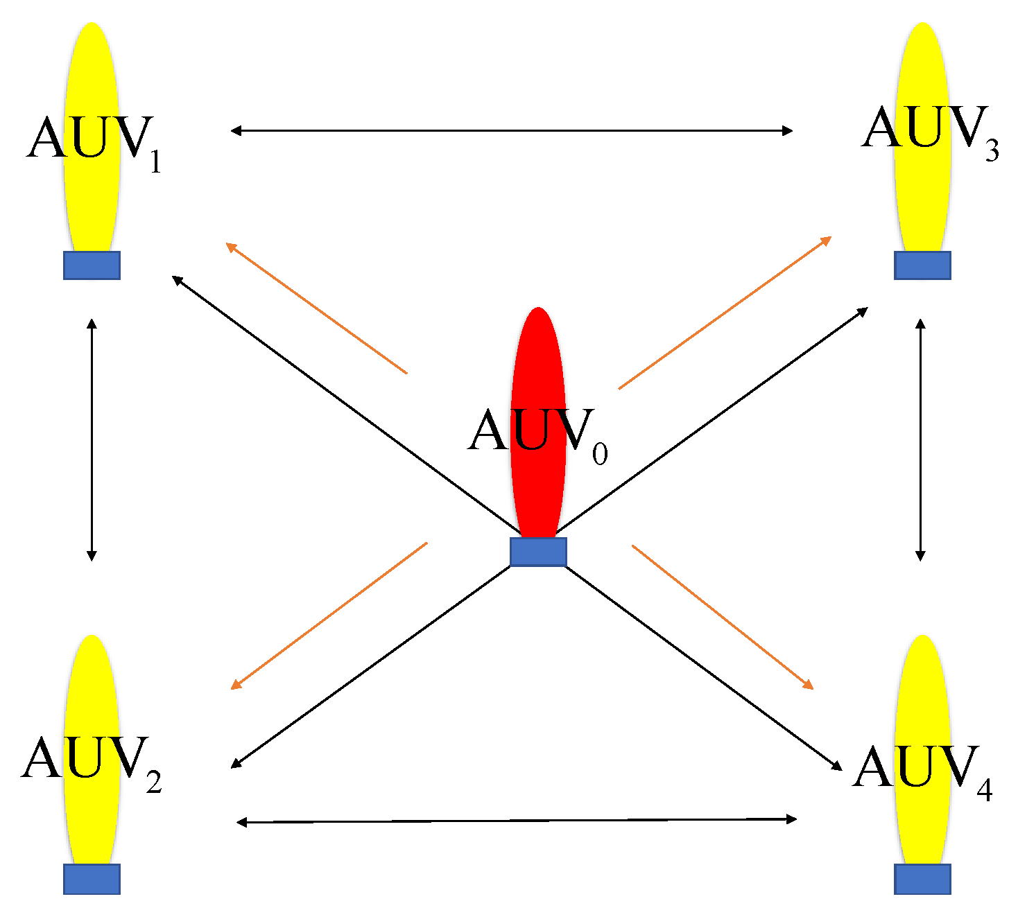
2.2. Graph Theory

The communication topology between AUVs can be described by a directed graph, which is an important basis for analyzing the communication relationship and communication quality in a multi-AUV system. Assume that there are n vehicles in a system, the directed graph $G=(\upsilon ,\epsilon ,A)$ consists of a node set $\upsilon =\{1,2,\dots ,n\}$, an edge set $\epsilon =\left\{\right(i,j\left)\right|i,j\in \upsilon \}\subseteq \upsilon \times \upsilon$, and the adjacency matrix $A=\left[a_{ij}\right]\in {\mathbb{R}}^{n\times n}$. In the communication graph of this system, it is defined that the communication weights between AUVs are the same. In A, $a_{ij}=1$ means that $\mathrm{AU}{\mathrm{V}}_i$ can receive the information from $\mathrm{AU}{\mathrm{V}}_j$ if and only if $(i,j)\in \epsilon$, $a_{ij}=0$ otherwise. The graph G is called strongly connected if $\mathrm{AU}{\mathrm{V}}_i$ can receive information from $\mathrm{AU}{\mathrm{V}}_j$ and $\mathrm{AU}{\mathrm{V}}_j$ can receive information from $\mathrm{AU}{\mathrm{V}}_i$$\forall (i,j)\in \epsilon$. Define the neighbor set of nodes i as $N_i=\{j\in \upsilon |(i,j)\in \epsilon \}$. The in-degree matrix is a diagonal matrix $D=diag(d_1^{in},d_2^{in},\dots ,d_n^{in})$, where $d_i^{in}={\sum }_{j=1}^n{a}_{ij}$ represents the number of vehicles whose information can be received by $\mathrm{AU}{\mathrm{V}}_i$. The Laplacian matrix is defined as $L=\left[l_{ij}\right]=D-A$. More information about graph theory can be obtained in [31].

The communication topology in this paper is divided into two parts. One is the communication topology $G_B$ between the leader $\mathrm{AU}{\mathrm{V}}_0$ and each follower $\mathrm{AU}{\mathrm{V}}_i$, and the other is the communication topology G between all the followers $\mathrm{AU}{\mathrm{V}}_i$. The matrix related to $G_B$ is defined as $B=diag(b_{10},b_{20},\dots ,b_{n0})$, where $b_{i0}=1$ if $\mathrm{AU}{\mathrm{V}}_i$ can receive information from $\mathrm{AU}{\mathrm{V}}_0$, and $b_{i0}=0$ indicates that $\mathrm{AU}{\mathrm{V}}_0$ does not send information to $\mathrm{AU}{\mathrm{V}}_i$.

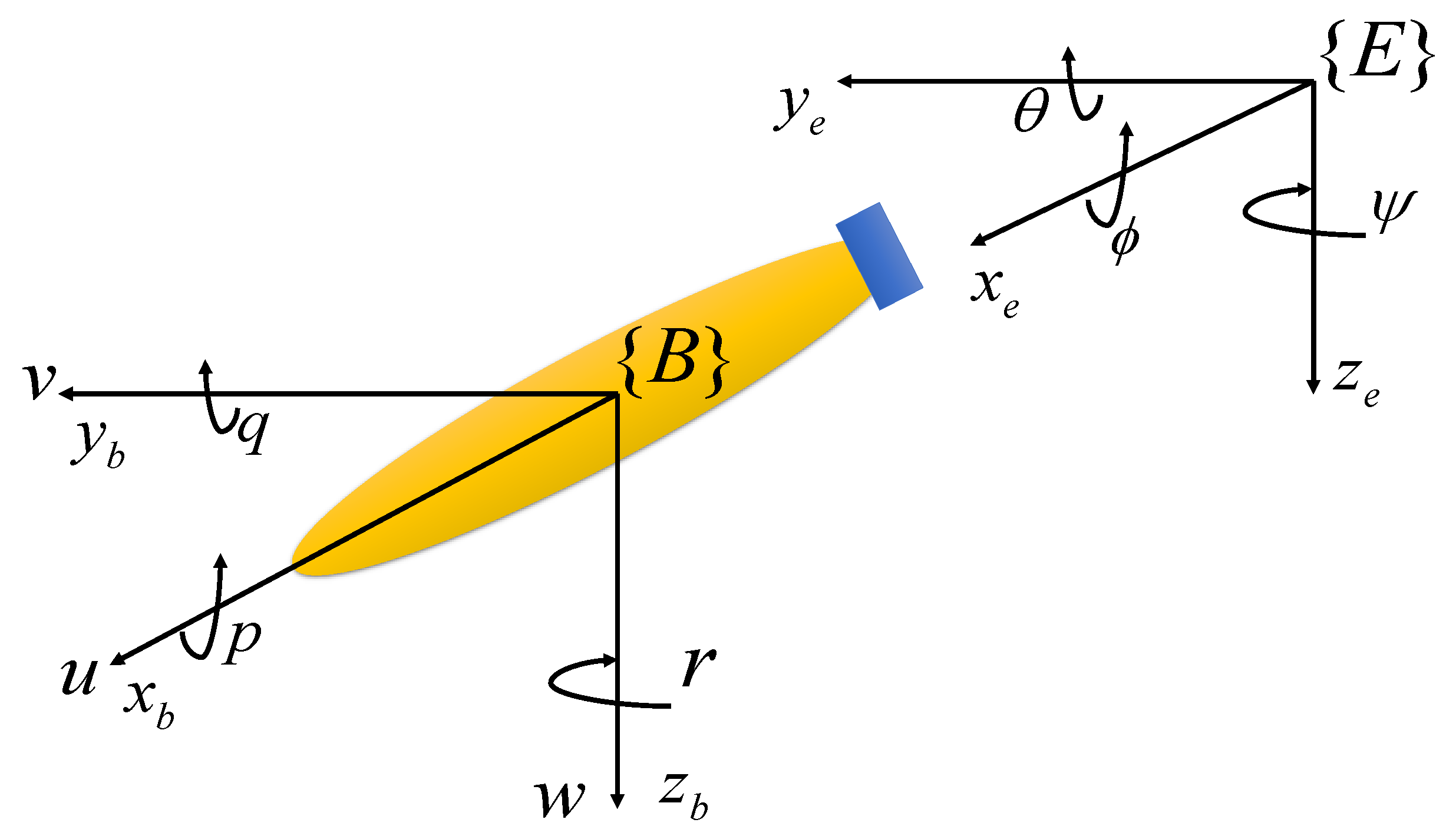
2.3. Feedback Linearization of AUV Model

The dynamic model of AUV can usually be described by six degrees of freedom (DOF) model according to the body-fixed $\left\{B\right\}$ and earth-fixed $\left\{E\right\}$ coordinate systems as shown in Figure 1. In most cases, the impact of roll on the AUV motion is very weak, so the nonlinear coupled kinematics and dynamics motion model with 5-DOF of the AUV that ignores the roll speed can be expressed as

$$\left\{\begin{array}{cc}\hfill & \dot{\mathit{\eta }}=\mathit{J}\left(\mathit{\eta }\right)\mathit{v}\hfill \\ \hfill & \mathit{M}\dot{\mathit{v}}+\mathit{C}\left(\mathit{v}\right)\mathit{v}+\mathit{D}\left(\mathit{v}\right)\mathit{v}+\mathit{g}\left(\mathit{\eta }\right)=\mathit{\tau }\hfill \end{array}\right.$$

(1)

where $\mathit{\eta }={[x_e,y_e,z_e,\theta ,\psi ]}^T\in {\mathbb{R}}^5$ represents the states of position and Euler angles for AUV, $\mathit{J}\left(\mathit{\eta }\right)$ is the rotational transformation matrix from body-fixed frame to earth-fixed frame, $\mathit{v}={[u_b,v_b,w_b,q,r]}^T\in {\mathbb{R}}^5$ is the velocity vector of AUV, $\mathit{M}$ is the inertia matrix, $\mathit{C}\left(\mathit{v}\right)$ is the Coriolis and centripetal matrix, $\mathit{D}\left(\mathit{v}\right)$ is the damping matrix, $\mathit{g}\left(\mathit{\eta }\right)$ is a vector of generalized gravitational and buoyancy forces and moments, and $\mathit{\tau }$ is the control inputs. More detailed parameters of the components of (1) are available in [32,33].

In this paper, the shape of the AUV is like the torpedo, and it is highly symmetrical in both the horizontal and vertical planes, which means that some complex parameters in the model can be simplified or even ignored, while $\mathit{g}\left(\mathit{\eta }\right)$ is equal to zero. Both the body-rigid part and hydrodynamic part for added mass are contained in matrix $\mathit{M}$ and $\mathit{C}\left(\mathit{v}\right)$, which have been described more specifically in [34].

The motion model of AUV can be derived as

$$\left[\begin{array}{c}\dot{\mathit{\eta }}\\ \dot{\mathit{v}}\end{array}\right]=\left[\begin{array}{cc}I& \mathit{0}\\ \mathit{0}& -{\mathit{M}}^{-1}\end{array}\right]\left[\begin{array}{c}\mathit{J}\left(\mathit{\eta }\right)\mathit{v}\\ \mathit{K}\left(\mathit{v}\right)\mathit{v}\end{array}\right]+\left[\begin{array}{c}\mathit{0}\\ {\mathit{M}}^{-1}\mathit{\gamma }\left(\mathit{\sigma }\right)\end{array}\right]\tilde{\mathit{u}}$$

(2)

where $\tilde{\mathit{u}}={\left[T_u,T_v,T_w,{\delta }_s,{\delta }_r\right]}^T$ represents propulsion forces of the AUV in three velocity directions and rudder angles on horizontal and vertical, $\mathit{\gamma }$ is the hydrodynamic coefficient matrix with respect to the rudder angles, and $\mathit{K}\left(\mathit{v}\right)=-\left(\mathit{C}\left(\mathit{v}\right)+\mathit{D}\left(\mathit{v}\right)+\mathit{g}\left(\mathit{\eta }\right){\tilde{\mathit{v}}}^T\right)$, where ${\tilde{\mathit{v}}}^T\mathit{v}=1$.

Based on (2), the standard nonlinear function of AUV model can be obtained as

$$\left\{\begin{array}{cc}\hfill & \dot{\mathit{\sigma }}=\tilde{f}\left(\mathit{\sigma }\right)+\tilde{g}\left(\mathit{\sigma }\right)\tilde{\mathit{u}}\hfill \\ \hfill & \mathit{\mu }=\tilde{h}\left(\mathit{\sigma }\right)\hfill \end{array}\right.$$

(3)

where $\mathit{\sigma }={[{\mathit{\eta }}^T,{\mathit{v}}^T]}^T$, $\tilde{f}\left(\mathit{\sigma }\right)={\left[{\tilde{f}}_i\left(\mathit{\sigma }\right)\right]}^T=\left[\begin{array}{cc}I& \mathit{0}\\ \mathit{0}& -{\mathit{M}}^{-1}\end{array}\right]\left[\begin{array}{c}\mathit{J}\left(\mathit{\eta }\right)\mathit{v}\\ \mathit{K}\left(\mathit{v}\right)\mathit{v}\end{array}\right],\begin{array}{c}\end{array}i=1,2,\dots ,10$, $\tilde{g}\left(\mathit{\sigma }\right)=\left[{\tilde{g}}_{ij}\left(\mathit{\sigma }\right)\right]=\left[\begin{array}{c}\mathit{0}\\ {\mathit{M}}^{-1}\mathit{\gamma }\left(\mathit{\sigma }\right)\end{array}\right],\begin{array}{c}\end{array}i,j=1,2,\dots ,10$, $\tilde{h}\left(\mathit{\sigma }\right)={\left[{\tilde{h}}_i\left(\mathit{\sigma }\right)\right]}^T=\mathit{\eta },\begin{array}{c}\end{array}i=1,2,\dots ,5$.

For the output $\tilde{h}\left(\mathit{\sigma }\right)$ in system (3), the Lie derivative of ${\tilde{h}}_i\left(\mathit{\sigma }\right)$ with respect to $\tilde{f}\left(\mathit{\sigma }\right)$ is expressed as $L_{\tilde{f}}{\tilde{h}}_i\left(\mathit{\sigma }\right)={\tilde{f}}_i\left(\mathit{\sigma }\right),\begin{array}{c}i=1,2,\dots ,5\end{array}$, then we can get the second-order Lie derivative of ${\tilde{h}}_i\left(\mathit{\sigma }\right)$ with respect to $\tilde{f}\left(\mathit{\sigma }\right)$: $L_{\tilde{f}}^2{\tilde{h}}_i\left(\mathit{\sigma }\right),i=1,2,\dots ,5$.

Two new vectors for $\mathrm{AU}{\mathrm{V}}_i$ are defined as

$$\left\{\begin{array}{cc}\hfill & {\mathit{x}}_i={[{\tilde{h}}_1\left(\mathit{\sigma }\right),{\tilde{h}}_2\left(\mathit{\sigma }\right),{\tilde{h}}_3\left(\mathit{\sigma }\right),{\tilde{h}}_4\left(\mathit{\sigma }\right),{\tilde{h}}_5\left(\mathit{\sigma }\right)]}^T\hfill \\ \hfill & {\mathit{v}}_i={[L_{\tilde{f}}{\tilde{h}}_1\left(\mathit{\sigma }\right),L_{\tilde{f}}{\tilde{h}}_2\left(\mathit{\sigma }\right),L_{\tilde{f}}{\tilde{h}}_3\left(\mathit{\sigma }\right),L_{\tilde{f}}{\tilde{h}}_4\left(\mathit{\sigma }\right),L_{\tilde{f}}{\tilde{h}}_5\left(\mathit{\sigma }\right)]}^T\hfill \end{array}\right.$$

(4)

Based on the above contents, the control input of the new linearization system is defined as

$${\mathit{u}}_i=\mathit{B}\left(\mathit{\sigma }\right)+\Gamma \left(\mathit{\sigma }\right)\tilde{\mathit{u}}$$

(5)

where $\mathit{B}\left(\mathit{\sigma }\right)={[L_{\tilde{f}}^2{\tilde{h}}_1\left(\mathit{\sigma }\right),L_{\tilde{f}}^2{\tilde{h}}_2\left(\mathit{\sigma }\right),L_{\tilde{f}}^2{\tilde{h}}_3\left(\mathit{\sigma }\right),L_{\tilde{f}}^2{\tilde{h}}_4\left(\mathit{\sigma }\right),L_{\tilde{f}}^2{\tilde{h}}_5\left(\mathit{\sigma }\right)]}^T$, $\Gamma \left(\mathit{\sigma }\right)=\left[L_{\tilde{g}j}{L}_{\tilde{f}}{\tilde{h}}_i\left(\mathit{\sigma }\right)\right]\in {\mathbb{R}}^{5\times 5}$. The actual AUV control input can be calculated as $\tilde{\mathit{u}}=\Gamma {\left(\mathit{\sigma }\right)}^{-1}(\mathit{u}-\mathit{B}\left(\mathit{\sigma }\right))$.

By combining (4) and (5), the standard second-order integrator dynamic of after feedback linearization can be obtained as

$$\left\{\begin{array}{cc}\hfill & {\dot{\mathit{x}}}_i={\mathit{v}}_i\hfill \\ \hfill & {\dot{\mathit{v}}}_i={\mathit{u}}_i\hfill \end{array}\right.$$

(6)

where ${\mathit{x}}_i\in {\mathbb{R}}^5,\begin{array}{c}\end{array}{\mathit{v}}_i\in {\mathbb{R}}^5,\begin{array}{c}\end{array}{\mathit{u}}_i\in {\mathbb{R}}^5,\begin{array}{c}\end{array}i=1,2,\dots ,n$.

2.4. Lemmas and Definitions

Lemma 1

([35]). The Kronecker product is an operation between two matrices represented by symbol ⊗, with the following properties:

(1)

$\left(kA\right)\otimes B=A\otimes \left(kB\right)$;

(2)

$(A+B)\otimes C=A\otimes C+B\otimes C$;

(3)

$(A\otimes B)(C\otimes D)=\left(AC\right)\otimes \left(BD\right)$.

Lemma 2

([36]). Let $M=\left[\begin{array}{cc}{A}_{11}& A_{12}\\ A_{21}& A_{22}\end{array}\right]$ and $A_{11},\begin{array}{c}\end{array}{A}_{12},\begin{array}{c}\end{array}{A}_{21},\begin{array}{c}\end{array}{A}_{22}\in {\mathbb{R}}^{n\times n}$. Then $det\left(M\right)=det(A_{11}{A}_{22}-A_{12}{A}_{21})$, if $A_{11},\begin{array}{c}\end{array}{A}_{12},\begin{array}{c}\end{array}{A}_{21}$ and $A_{22}$ commute pairwise.

Lemma 3

([37]). Polynomial $Q\left(z\right)$ (of degree d) is Schur stable if and only if polynomial $R\left(z\right)$ is Hurwitz stable, where $R\left(z\right)={(z-1)}^{d}Q\left(\frac{z+1}{z-1}\right)$. For a complex polynomial $R\left(z\right)$, let $R\left(\mathrm{i}\omega \right)=m\left(\omega \right)+\mathrm{i}n\left(\omega \right)$, where $m\left(\omega \right),\begin{array}{c}\end{array}n\left(\omega \right)\in \mathbb{R}$, and $\mathrm{i}$ is the imaginary unit.

Definition 1

([38]). The polynomial $m\left(\omega \right),\begin{array}{c}\end{array}n\left(\omega \right)$ is interlaced, if the following two statements are satisfied.

(1)

$m\left(\omega \right)=0,\begin{array}{c}\end{array}n\left(\omega \right)=0$ only have distinct real roots, respectively, $m_1<m_2<\dots <m_l$, $n_1<n_2<\dots <n_{l^{\prime }}$;

(2)

$\left|l-l^{\prime }\right|\le 1$ and the roots of $m\left(\omega \right)=0,\begin{array}{c}\end{array}n\left(\omega \right)=0$ satisfy one of the following four cases:

(a)

$m_1<n_1<m_2<n_2<\dots <n_l^{\prime }<m_l,\begin{array}{c}\end{array}l=l^{\prime }+1$;

(b)

$n_1<m_1<n_2<m_2<\dots <m_l^{\prime }<n_l,\begin{array}{c}\end{array}{l}^{\prime }=l+1$;

(c)

$m_1<n_1<m_2<n_2<\dots <n_l^{\prime }<m_l,\begin{array}{c}\end{array}l=l^{\prime }$;

(d)

$n_1<m_1<n_2<m_2<\dots <m_l^{\prime }<n_l,\begin{array}{c}\end{array}l=l^{\prime }$.

Lemma 4

([38,39]). The complex polynomial $R\left(z\right)$ is Hurwitz stable if and only if the related pair $m\left(\omega \right)$ and $n\left(\omega \right)$ is interlaced, and $m\left(0\right)n^{\prime }\left(0\right)-m^{\prime }\left(0\right)n\left(0\right)>0$.

3. Main Results

In actual engineering applications, continuous information exchange between AUVs is difficult to achieve, so we consider the discrete-time coordinated control of the multi-AUV system. By using the forward difference method for (6), the discrete-time dynamics of $\mathrm{AU}{\mathrm{V}}_i$ can be obtained as

$$\left\{\begin{array}{cc}\hfill & {\mathit{x}}_i(k+1)={\mathit{x}}_i\left(k\right)+T{\mathit{v}}_i\left(k\right)\hfill \\ \hfill & {\mathit{v}}_i(k+1)={\mathit{v}}_i\left(k\right)+T{\mathit{u}}_i\left(k\right)\hfill \end{array}\right.$$

(7)

where k represents the discrete-time index and T is the sampling period. ${\mathit{x}}_i\left(k\right)\in {\mathbb{R}}^5$, ${\mathit{v}}_i\left(k\right)\in {\mathbb{R}}^5$ are the linearization position and velocity states of $\mathrm{AU}{\mathrm{V}}_i$ at $t=kT$.

According to Equation (7), the dynamics of leader $\mathrm{AU}{\mathrm{V}}_0$ and follower $\mathrm{AU}{\mathrm{V}}_i$ can be described as the following two forms (see Equations (7) and (8)):

$$x_0(k+1)=x_0\left(k\right)+T{v}_0\left(k\right)$$

(8)

where $x_i\in \mathbb{R}$ and $v_i\in \mathbb{R}$ are the corresponding individual elements in ${\mathit{x}}_i\in {\mathbb{R}}^5$ and ${\mathit{v}}_i\in {\mathbb{R}}^5$, respectively. $u_i\in \mathbb{R}$ is the element in ${\mathit{u}}_i\in {\mathbb{R}}^5$ that corresponds to $x_i$.

Definition 2.

The coordinated formation of multi-AUV system is achieved if the following two equations are satisfied:

$$\left\{\begin{array}{cc}& \underset{k\to \infty }{lim}∥x_i\left(k\right)-x_0\left(k\right)∥=0,i\in \upsilon \hfill \\ & \underset{k\to \infty }{lim}∥v_i\left(k\right)-v_0\left(k\right)∥=0,i\in \upsilon \hfill \end{array}\right.$$

Remark 1.

Suppose the position difference between $\mathrm{AU}{\mathrm{V}}_0$ and $\mathrm{AU}{\mathrm{V}}_i$ in the desired formation is ${\Delta }_i=x_i^d-x_0$, let $x_i=x_i^d-{\Delta }_i$, so $x_i=x_0$, i.e., the position and velocity states of $\mathrm{AU}{\mathrm{V}}_0$ and $\mathrm{AU}{\mathrm{V}}_i$ achieve consensus, so are the states of all followers. Therefore, the multi-AUV system achieves consensus. In addition, by setting ${\Delta }_i$ to be time-varying, time-varying formation control can be performed.

3.1. Coordinated Formation Control without Communication Delay

To solve the dynamic consensus problem for multi-AUV system with sampled information, the coordinated controller can be designed as

$$\begin{array}{cc}\hfill u_i\left(k\right)=& \alpha b_{i0}\left(k\right)(x_0\left(k\right)-x_i\left(k\right))+\beta b_{i0}\left(k\right)(v_0\left(k\right)-v_i\left(k\right))\hfill \\ \hfill & +\alpha \sum _{j\in N_i}{a}_{ij}\left(k\right)(x_j\left(k\right)-x_i\left(k\right))+\beta \sum _{j\in N_i}{a}_{ij}\left(k\right)(v_j\left(k\right)-v_i\left(k\right))\hfill \end{array}$$

(9)

where $\alpha$ and $\beta$ represent the position and velocity control gains, $b_{i0}\left(k\right)$ and $a_{ij}\left(k\right)$ are the elements in the matrices B and A related to communication topologies $G_B$ and G.

Define the position error and velocity error between $\mathrm{AU}{\mathrm{V}}_0$ and $\mathrm{AU}{\mathrm{V}}_i$ at $t=kT$ as $e_i\left(k\right)=x_i\left(k\right)-x_0\left(k\right)$, $f_i\left(k\right)=v_i\left(k\right)-v_0\left(k\right)$, respectively. The multiple errors vectors can be expressed as

$$\left\{\begin{array}{cc}& \mathit{E}\left(k\right)={\left[e_1\left(k\right),e_2\left(k\right),e_3\left(k\right),\dots ,e_n\left(k\right)\right]}^T\hfill \\ & \mathit{F}\left(k\right)={\left[f_1\left(k\right),f_2\left(k\right),f_3\left(k\right),\dots ,f_n\left(k\right)\right]}^T\hfill \end{array}\right.$$

where $\mathit{E}\left(k\right)\in {\mathbb{R}}^n,\begin{array}{c}\end{array}\mathit{F}\left(k\right)\in {\mathbb{R}}^n$.

By combining (7)–(9), we can build a discrete-time error system as

$$\left[\begin{array}{c}\mathit{E}(k+1)\\ \mathit{F}(k+1)\end{array}\right]=\mathit{P}\left[\begin{array}{c}\mathit{E}\left(k\right)\\ \mathit{F}\left(k\right)\end{array}\right]$$

(10)

with

$$\mathit{P}=\left[\begin{array}{cc}{I}_n& T{I}_n\\ -\alpha T(B_k+L_k)& I_n-\beta T(B_k+L_k)\end{array}\right]$$

where $B_k$, $L_k$ respectively represent B and L at $t=kT$.

Remark 2.

By using the Kronecker product ⊗ and Lemma 1, the error system for all states in the multi-AUV system can be derived on the basis of (10), and the stability analysis is the same as that of (10).

Lemma 5.

The multi-AUV system under controller (9) achieves consensus asymptotically if and only if $\rho \left(\mathit{P}\right)<1$.

Remark 3.

It can be observed from the definitions of $e_i\left(k\right)$ and $f_i\left(k\right)$ that the multi-AUV system under coordinated controller (9) can achieve consensus asymptotically if and only if the discrete-time error system (10) is globally asymptotically stable.

Theorem 1.

For communication topology $G_B$ and G, controller gains α and β, and sampling period T, the consensus of the multi-AUV system can be achieved, i.e., the problem of coordinated formation control of multiple AUVs can be solved, if and only if the follows projects are satisfied:

$${\Theta }_1>0$$

(11)

$${\Theta }_1{\left({\Theta }_2\right)}^2{\Theta }_3+{\Theta }_4>0$$

(12)

$${\Theta }_2>0$$

(13)

where ${\Theta }_1=T\left(\alpha T-2\beta \right){\left|{\lambda }_i\right|}^2+4Re\left({\lambda }_i\right)$, ${\Theta }_2=\beta -\alpha T$, ${\Theta }_3={\left|{\lambda }_i\right|}^2$, ${\Theta }_4=-4\alpha {Im}^2\left({\lambda }_i\right)$, and ${\lambda }_i,\begin{array}{c}\end{array}i=1,2,3,\dots ,n$ is the eigenvalue of matrix $(B_k+L_k)$.

Proof. 

According to Lemma 2, we can get

$$\begin{array}{cc}\hfill det\left(s{I}_{2n}-\mathit{P}\right)& =det\left[\begin{array}{cc}\begin{array}{c}\left(s-1\right)I_n\\ \alpha T(B_k+L_k)\end{array}& \begin{array}{c}-T{I}_n\\ \left(s-1\right)I_n+\beta T(B_k+L_k)\end{array}\end{array}\right]\hfill \\ & =\prod _{i=1}^n\left[s^2+\left(\beta T{\lambda }_i-2\right)s+\alpha T^2{\lambda }_i-\beta T{\lambda }_i+1\right]\hfill \end{array}$$

Let $Q_i\left(s\right)=s^2+\left(\beta T{\lambda }_i-2\right)s+\alpha T^2{\lambda }_i-\beta T{\lambda }_i+1,i=1,2,\dots ,n$. If $Q_i\left(s\right)$ are Schur stable, for $i=1,2,\dots ,n$, ${\lambda }_i$ cannot be zero.

Then let

$$\begin{array}{cc}\hfill R_i\left(\xi \right)& ={\left(\xi -1\right)}^2{Q}_i\left(\frac{\xi +1}{\xi -1}\right)\hfill \\ & =\alpha T^2{\lambda }_i{\xi }^2+2\left(\beta T{\lambda }_i-\alpha T^2{\lambda }_i\right){\lambda }_i\xi +\alpha T^2{\lambda }_i-2\beta T{\lambda }_i+4\hfill \end{array}$$

and

$$\begin{array}{cc}\hfill {\widehat{R}}_i\left(\xi \right)& =\frac{R_i\left(\xi \right)}{\alpha T^2{\lambda }_i}\hfill \\ & ={\xi }^2+2\left(\frac{\beta }{\alpha T}-1\right)\xi +1-\frac{2\beta }{\alpha T}+\frac{4}{\alpha T^2{\lambda }_i}\hfill \end{array}$$

The same stability characteristics of $R_i\left(\xi \right)$ and ${\widehat{R}}_i\left(\xi \right)$ can be recognized without difficulty.

According to Lemma 3, polynomials $Q_i\left(s\right)$, for $i=1,2,3,\dots ,n$, are Schur stable if and only if polynomials ${\widehat{R}}_i\left(\xi \right)$, for $i=1,2,3,\dots ,n$, are Hurwitz stable.

For complex polynomial ${\widehat{R}}_i\left(\xi \right)$, let $\xi =\mathrm{i}\omega$, then we can obtain ${\widehat{R}}_i\left(\mathrm{i}\omega \right)=-{\omega }^2+1-\frac{2\beta }{\alpha T}+\frac{4Re\left({\lambda }_i\right)}{\alpha T^2{\left|{\lambda }_i\right|}^2}+\mathrm{i}\left[2\left(\frac{\beta }{\alpha T}-1\right)\omega -\frac{4Im\left({\lambda }_i\right)}{\alpha T^2{\left|{\lambda }_i\right|}^2}\right]$, so $m_i\left(\omega \right)=-{\omega }^2+1-\frac{2\beta }{\alpha T}+\frac{4Re\left({\lambda }_i\right)}{\alpha T^2{\left|{\lambda }_i\right|}^2}$ and $n_i\left(\omega \right)=2\left(\frac{\beta }{\alpha T}-1\right)\omega -\frac{4Im\left({\lambda }_i\right)}{\alpha T^2{\left|{\lambda }_i\right|}^2}$. Subsequently, according to Definition 1 and Lemma 4, ${\widehat{R}}_i\left(\xi \right)$ is Hurwitz stable if and only if the following conditions hold:

(1)

$m_i\left(\omega \right)=0$ has two distinct real roots $m_{i1}<m_{i2}$;

(2)

$m_{i1}<n_{i1}<m_{i2}$, where $n_{i1}$ is the only root of $n_i\left(\omega \right)=0$;

(3)

$m_i\left(0\right)n_i^{\prime }\left(0\right)-m_i^{\prime }\left(0\right)n_i\left(0\right)>0$.

Consider condition (1). $m_i\left(\omega \right)=0$ has two distinct real roots when and only when

$${\Delta }_m=1-\frac{2\beta }{\alpha T}+\frac{4Re\left({\lambda }_i\right)}{\alpha T^2{\left|{\lambda }_i\right|}^2}>0\iff T\left(\alpha T-2\beta \right){\left|{\lambda }_i\right|}^2+4Re\left({\lambda }_i\right)>0$$

(14)

And we can get the two distinct real roots as: $m_{i1}=-\sqrt{{\Delta }_m}$, $m_{i2}=\sqrt{{\Delta }_m}$.

Consider condition (2). The root of $n_i\left(\omega \right)=0$ can be obtained as $n_{i1}=\frac{2Im\left({\lambda }_i\right)}{T\left(\beta -\alpha T\right){\left|{\lambda }_i\right|}^2}$

Then we can get

$$\begin{array}{cc}\hfill m_{i1}<n_{i1}<m_{i2}& \iff -\sqrt{{\Delta }_m}<\frac{2Im\left({\lambda }_i\right)}{T\left(\beta -\alpha T\right){\left|{\lambda }_i\right|}^2}<\sqrt{{\Delta }_m}\hfill \\ \hfill & \iff \left[T\left(\alpha T-2\beta \right){\left|{\lambda }_i\right|}^2+4Re\left({\lambda }_i\right)\right]{\left(\beta -\alpha T\right)}^2{\left|{\lambda }_i\right|}^2-4\alpha {Im}^2\left({\lambda }_i\right)>0\hfill \end{array}$$

(15)

Consider condition (3). The components in the inequality can be obtained as: $m_i\left(0\right)=1-\frac{2\beta }{\alpha T}+\frac{4Re\left({\lambda }_i\right)}{\alpha T^2{\left|{\lambda }_i\right|}^2}$, ${n^{\prime }}_i\left(0\right)=2\left(\frac{\beta }{\alpha T}-1\right)$, ${m^{\prime }}_i\left(0\right)=0$, $n_i\left(0\right)=-\frac{4Im\left({\lambda }_i\right)}{\alpha T^2{\left|{\lambda }_i\right|}^2}$.

Then we can get

$$\begin{array}{cc}\hfill & m_i\left(0\right){n^{\prime }}_i\left(0\right)-{m^{\prime }}_i\left(0\right)n_i\left(0\right)>0\hfill \\ \hfill & \iff \left[T\left(\alpha T-2\beta \right){\left|{\lambda }_i\right|}^2+4Re\left({\lambda }_i\right)\right]\left(\beta -\alpha T\right)>0\hfill \end{array}$$

(16)

Finally, the three inequalities (11)–(13) in the Theorem 1 can be obtained from (14)–(16) respectively, and the proof is thus completed. □

Remark 4.

In order to ensure highly efficient coordinated control during the operation of multiple AUVs, the related matrix of communication topology $G_B$ should be $B=diag(1,1,\dots ,1)\in {\mathbb{R}}^{n\times n}$, and communication topology G should be strongly connected, i.e., all followers can receive messages from the leader and all followers can send and receive messages to and from each other. However, this ideal communication topology is difficult to achieve if there are a large number of AUVs in the formation and if the communication equipment of vehicles is accidentally damaged. Therefore, according to Theorem 1, a suitable and alterable communication topology can be obtained to solve the above problems, and the appropriate range of control gains and sampling period can be obtained.

3.2. Coordinated Formation Control with Time-Varying Communication Delay

Consider the time-varying communication delay ∂ between AUVs, the coordinated controller can be designed as

$$\begin{array}{cc}\hfill u_i\left(k\right)=& \alpha b_{i0}(k-d)(x_0(k-d)-x_i\left(k\right))+\beta b_{i0}(k-d)(v_0(k-d)-v_i\left(k\right))\hfill \\ \hfill & +\alpha \sum _{j\in N_i}{a}_{ij}(k-d)(x_j(k-d)-x_i\left(k\right))+\beta \sum _{j\in N_i}{a}_{ij}(k-d)(v_j(k-d)-v_i\left(k\right))\hfill \\ \hfill & +\alpha dT(b_{i0}(k-d)+\sum _{j\in N_i}{a}_{ij}(k-d))v_i(k-d)\hfill \end{array}$$

(17)

where d is a time-varying positive integer and $(d-1)T<\partial \le dT$.

By combining (7), (8) and (17), we can get a new discrete-time error system as

$$\left[\begin{array}{c}\mathit{E}(k+1)\\ \mathit{F}(k+1)\end{array}\right]=\mathit{S}\left[\begin{array}{c}\mathit{E}(k-d)\\ \mathit{F}(k-d)\end{array}\right]$$

(18)

with

$$\mathit{S}=\left[\begin{array}{cc}{I}_n& \widehat{d}T{I}_n\\ -\alpha T(B_{k-d}+L_{k-d})& I_n-\beta T(B_{k-d}+L_{k-d})\end{array}\right]$$

where $\widehat{d}=d+1$, $B_{k-d}$ and $L_{k-d}$ respectively represent B and L at time $t=(k-d)T$.

Remark 5.

In (17), there exist communication delays ∂, and we assume it is bounded $(d_m\le d\le d_M)$, so each follower $\mathrm{AU}{\mathrm{V}}_i$ actually receives the information from the leader $\mathrm{AU}{\mathrm{V}}_0$ or other follower $\mathrm{AU}{\mathrm{V}}_i$ from time $t=(k-d)T$. In (19), since d is dynamically varying, matrix $\mathit{S}$ is an interval matrix and can be expressed as $\mathit{S}\in [{\mathit{S}}^m,{\mathit{S}}^M]$. And $[{\mathit{S}}^m,{\mathit{S}}^M]=\{\mathit{S}=\left[s_{ij}\right]:s_{ij}^m\le s_{ij}\le s_{ij}^M,i,j=1,2,\dots ,n\}$.

Lemma 6.

The multi-AUV system under controller (17) achieves consensus asymptotically if and only if $\rho \left(\mathit{S}\right)<1$.

Lemma 7.

For all $\mathit{S}\in [{\mathit{S}}^m,{\mathit{S}}^M]$, if $\mathit{S}$ is Schur stable, we say that $[{\mathit{S}}^m,{\mathit{S}}^M]$ is Schur stable, i.e., the system (18) asymptotically stable.

Theorem 2.

For multi-AUV system with time-varying communication delay $(d-1)T<\partial \le dT$, the problem of coordinated formation control of multiple AUVs can be solved if and only if the follows projects are satisfied:

$${\Theta }_1^d>0$$

(19)

$${\Theta }_1^d{\left({\Theta }_2^d\right)}^2{\Theta }_3^d+{\Theta }_4^d>0$$

(20)

$${\Theta }_2^d>0$$

(21)

where ${\Theta }_1^d=T\left(\widehat{d}\alpha T-2\beta \right){\left|{\lambda }_i\right|}^2+4Re\left({\lambda }_i\right)$, ${\Theta }_2^d=\beta -\widehat{d}\alpha T$, ${\Theta }_3^d={\left|{\lambda }_i\right|}^2$, ${\Theta }_4^d=-4\widehat{d}\alpha {Im}^2\left({\lambda }_i\right)$, ${\lambda }_i,\begin{array}{c}\end{array}i=1,2,3,\dots ,n$ is the eigenvalue of matrix $(B_{k-d}+L_{k-d})$.

Proof. 

Similar to the proof in Theorem 1, there is

$$\begin{array}{cc}\hfill det(s{I}_{2n}-\mathit{S})& =det\left[\begin{array}{cc}\begin{array}{c}\left(s-1\right)I_n\\ \alpha T(B_k+L_k)\end{array}& \begin{array}{c}-\widehat{d}T{I}_n\\ \left(s-1\right)I_n+\beta T(B_k+L_k)\end{array}\end{array}\right]\hfill \\ \hfill & ={\prod }_{i=1}^n\left[s^2+\left(\beta T{\lambda }_i-2\right)s+\widehat{d}\alpha T^2{\lambda }_i-\beta T{\lambda }_i+1\right]\hfill \end{array}$$

Let $Q_i\left(s\right)=s^2+\left(\beta T{\lambda }_i-2\right)s+\widehat{d}\alpha T^2{\lambda }_i-\beta T{\lambda }_i+1,i=1,2,\dots ,n$, and ${\lambda }_i\ne 0$.

Then, let

$$\begin{array}{cc}\hfill R_i\left(\xi \right)& ={(\xi -1)}^2{Q}_i\left(\frac{\xi +1}{\xi -1}\right)\hfill \\ & =\widehat{d}\alpha T^2{\lambda }_i{\xi }^2+2\left(\beta T{\lambda }_i-\widehat{d}\alpha T^2{\lambda }_i\right){\lambda }_i\xi +\widehat{d}\alpha T^2{\lambda }_i-2\beta T{\lambda }_i+4\hfill \end{array}$$

and

$$\begin{array}{cc}\hfill {\widehat{R}}_i\left(\xi \right)& =\frac{R_i\left(\xi \right)}{\widehat{d}\alpha T^2{\lambda }_i}\hfill \\ & ={\xi }^2+2\left(\frac{\beta }{\widehat{d}\alpha T}-1\right)\xi +1-\frac{2\beta }{\widehat{d}\alpha T}+\frac{4}{\widehat{d}\alpha T^2{\lambda }_i}\hfill \end{array}$$

So the complex polynomial ${\widehat{R}}_i\left(\xi \right)$ can be expressed as

$$\begin{array}{cc}\hfill {\widehat{R}}_i\left(\xi \right)& ={\widehat{R}}_i\left(\mathrm{i}\omega \right)=m_i\left(\omega \right)+\mathrm{i}{n}_i\left(\omega \right)\hfill \\ \hfill & =-{\omega }^2+1-\frac{2\beta }{\widehat{d}\alpha T}+\frac{4Re\left({\lambda }_i\right)}{\widehat{d}\alpha T^2{\left|{\lambda }_i\right|}^2}+\mathrm{i}\left[2\left(\frac{\beta }{\widehat{d}\alpha T}-1\right)\omega -\frac{4Im\left({\lambda }_i\right)}{\widehat{d}\alpha T^2{\left|{\lambda }_i\right|}^2}\right]\hfill \end{array}$$

According to Lemmas 3 and 4, polynomials $Q_i\left(s\right)$, for $i=1,2,3,\dots ,n$, are Schur stable if and only if the following conditions hold:

(1)

$m_i\left(\omega \right)=0$ has two distinct real roots $m_{i1}<m_{i2}$;

(2)

$m_{i1}<n_{i1}<m_{i2}$;

(3)

$m_i\left(0\right)n_i^{\prime }\left(0\right)-m_i^{\prime }\left(0\right)n_i\left(0\right)>0$.

Finally, we can obtain the three inequalities (19)–(21) in Theorem 2 by considering the three conditions (1)–(3), respectively. The proof is completed. □

Remark 6.

In this paper, the communication delay is bounded, so we know the values of $d_m$ and $d_M$. Therefore, suitable controller parameters based on the delay variation interval can be obtained.

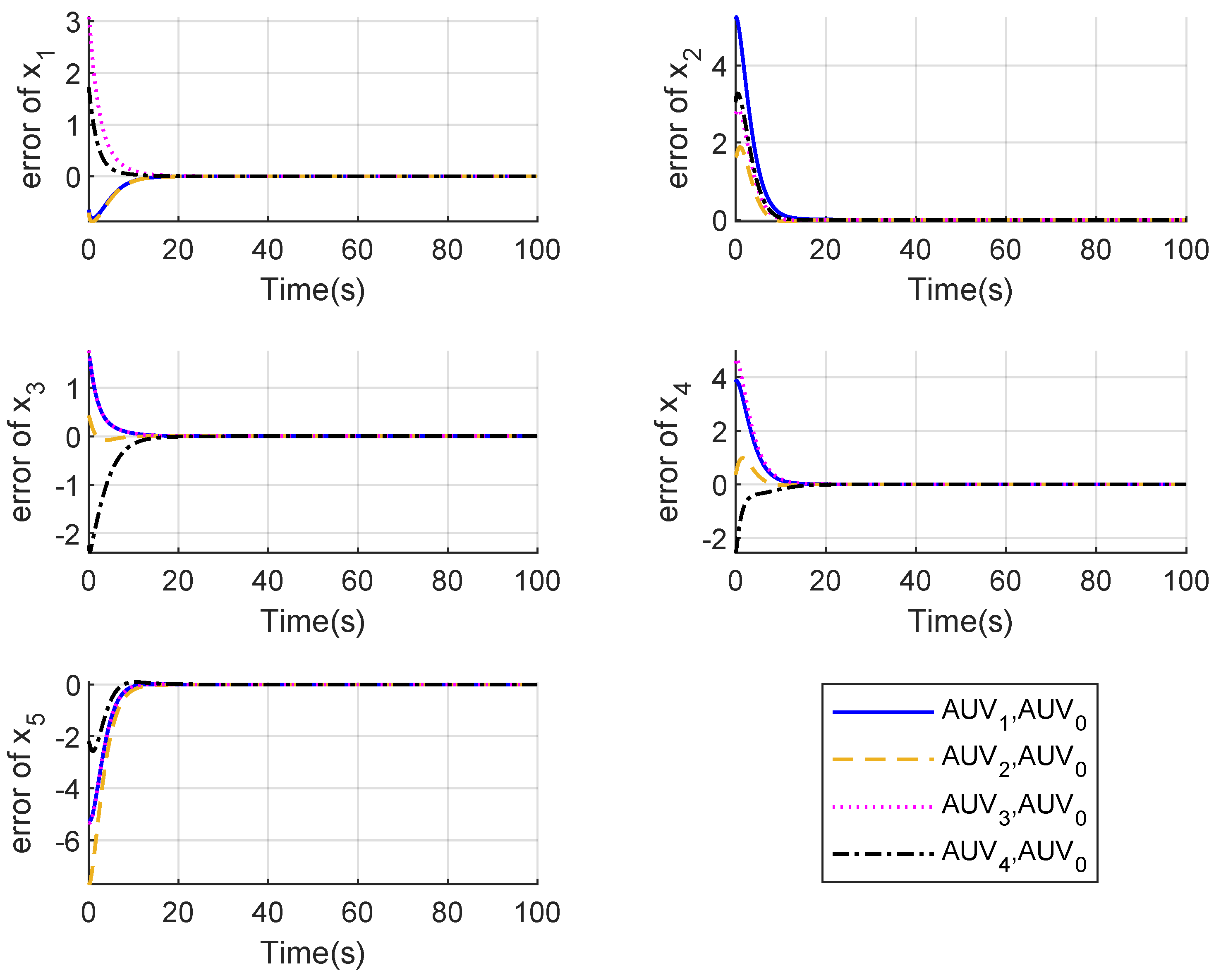
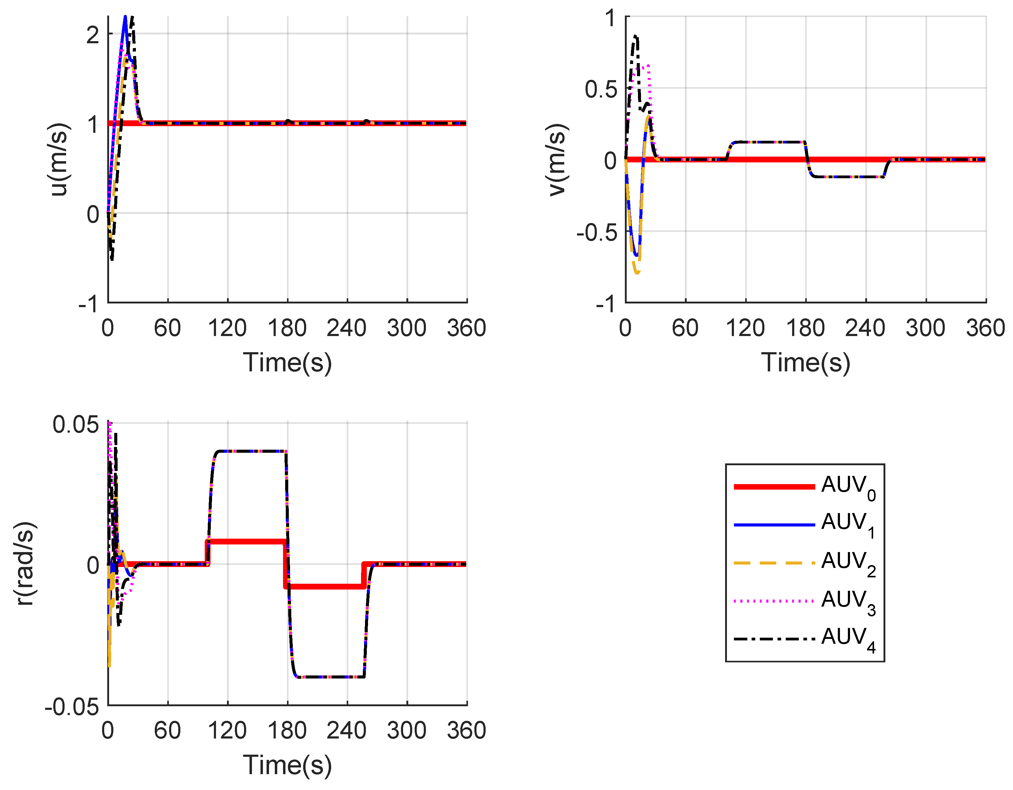
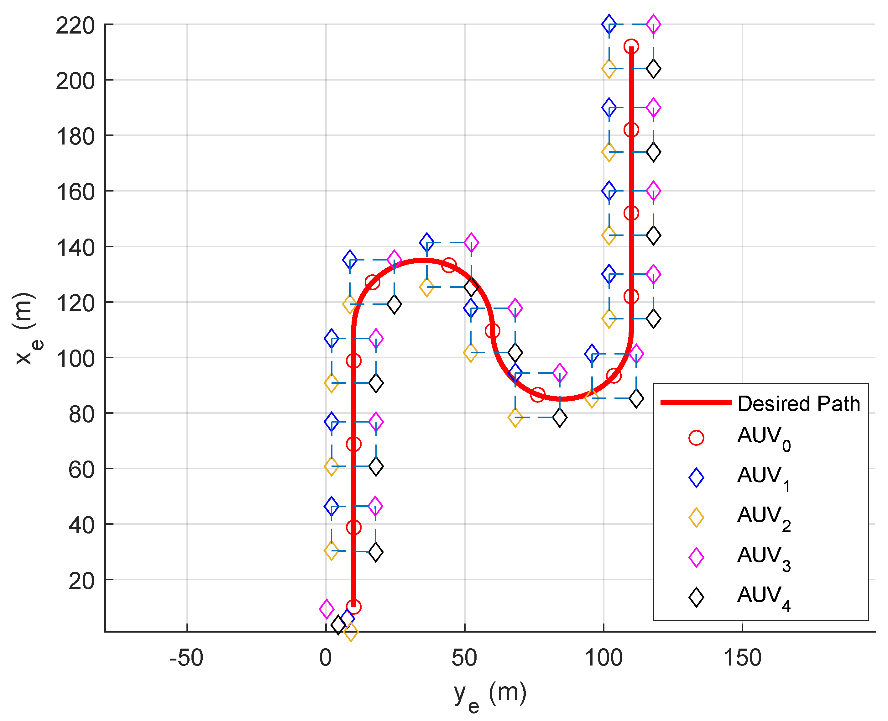
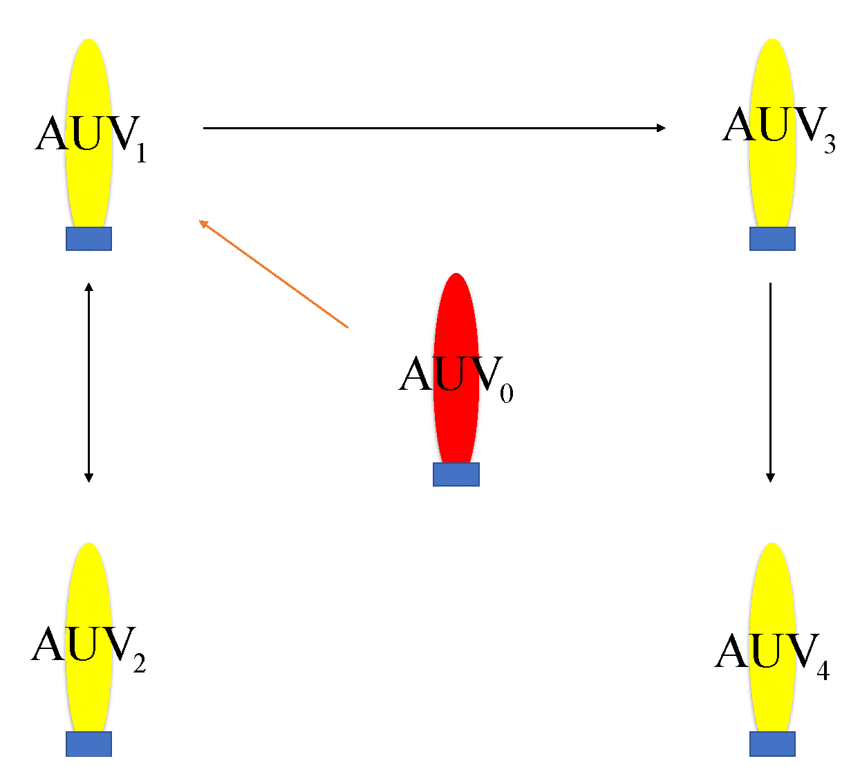
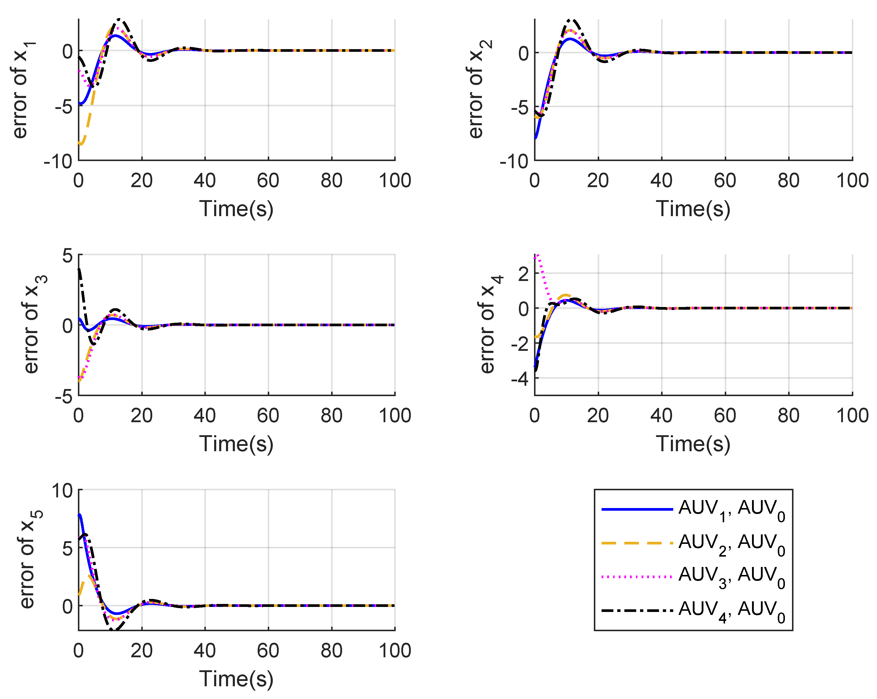
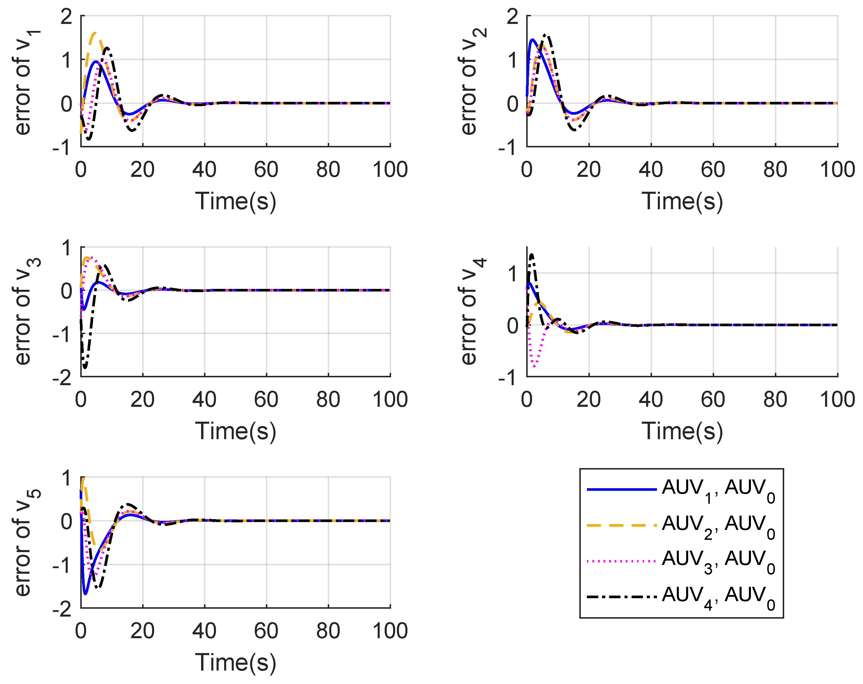
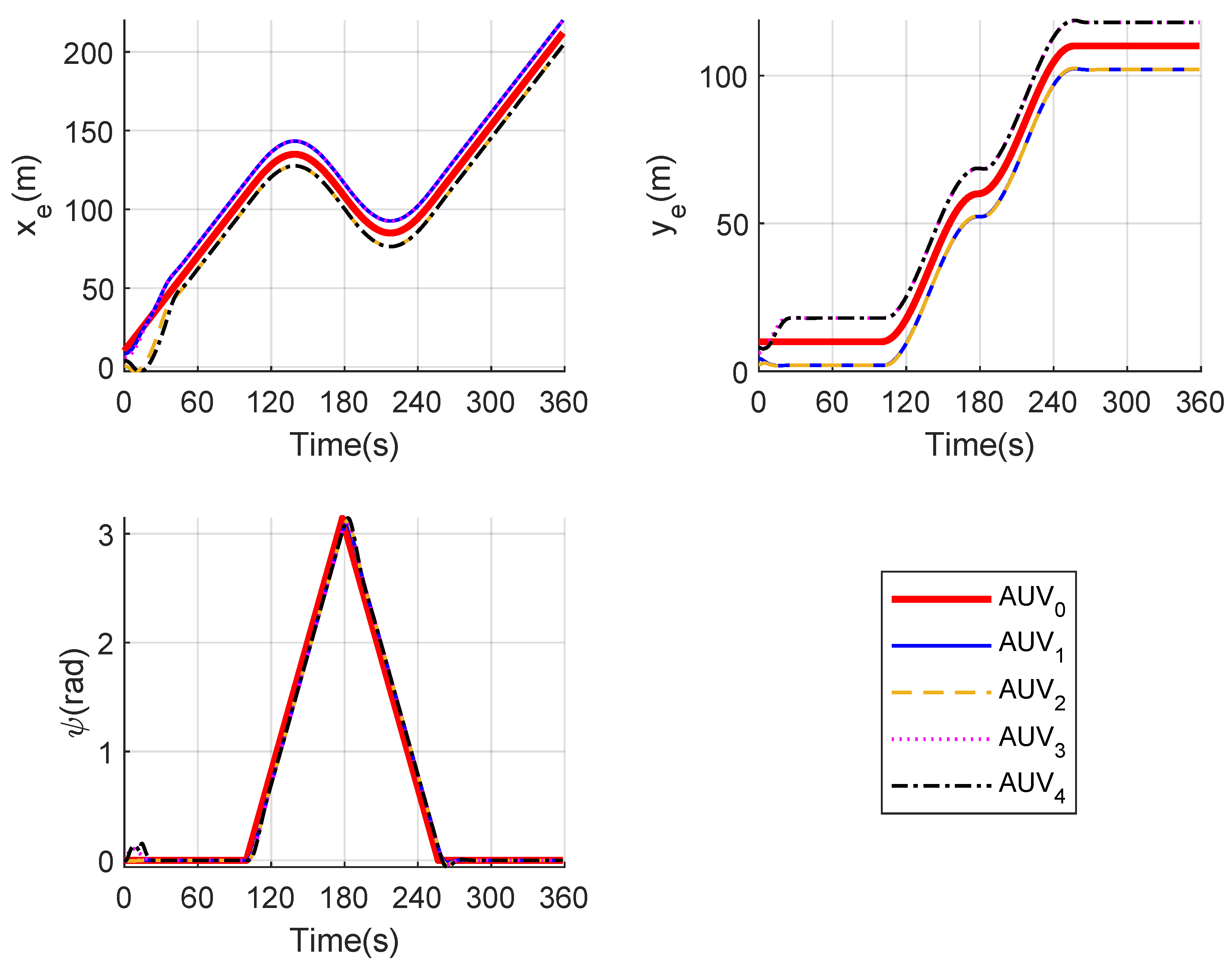
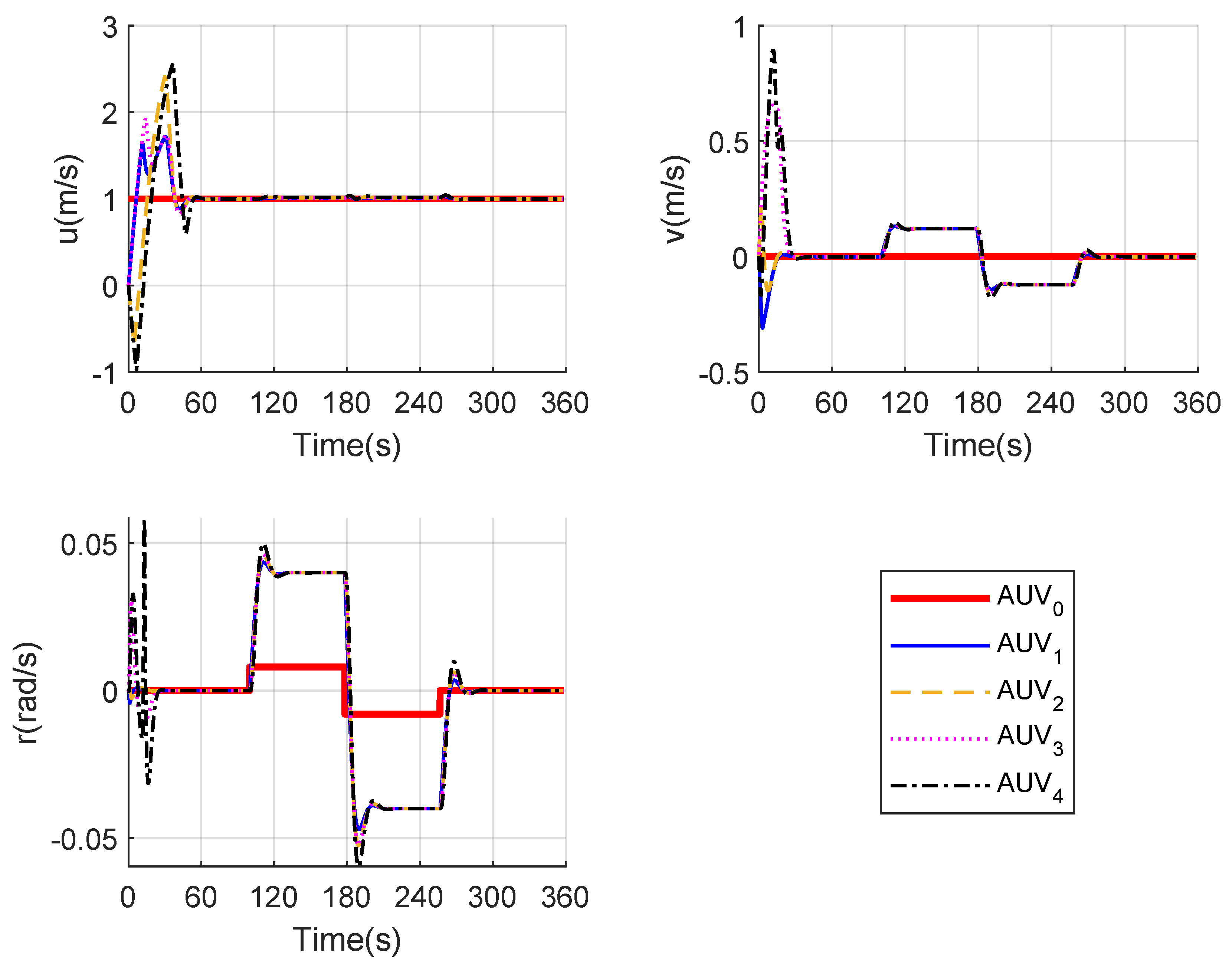
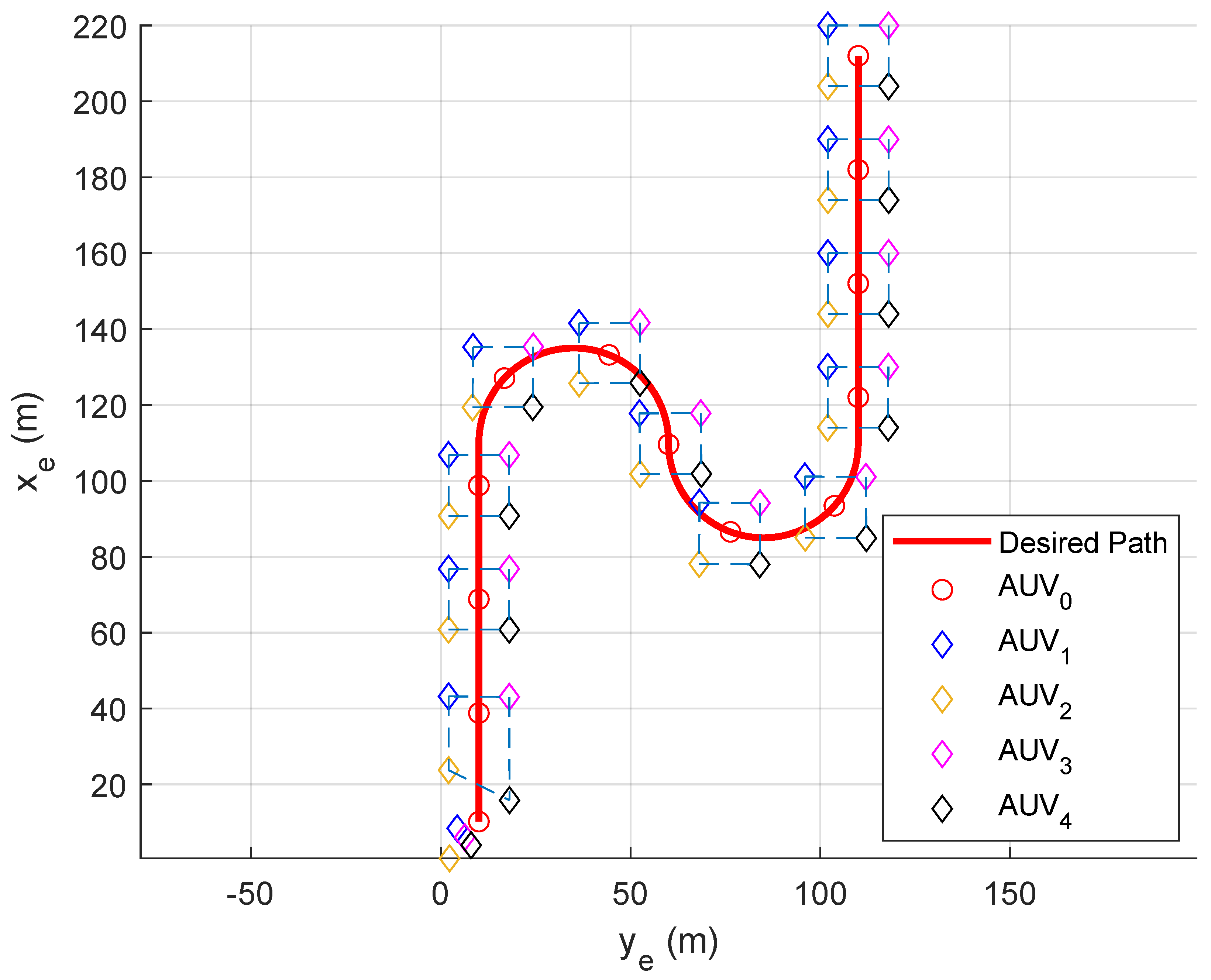
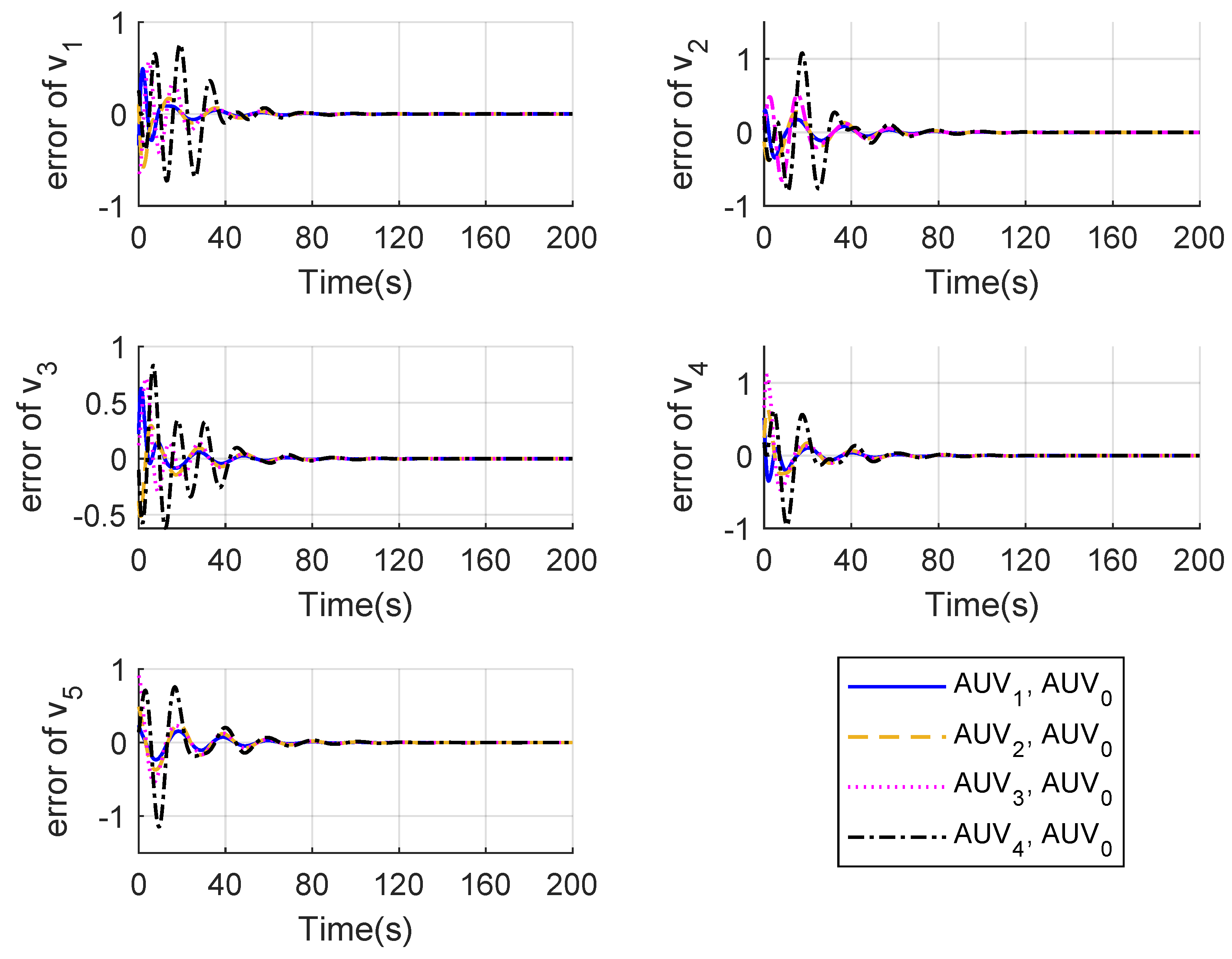
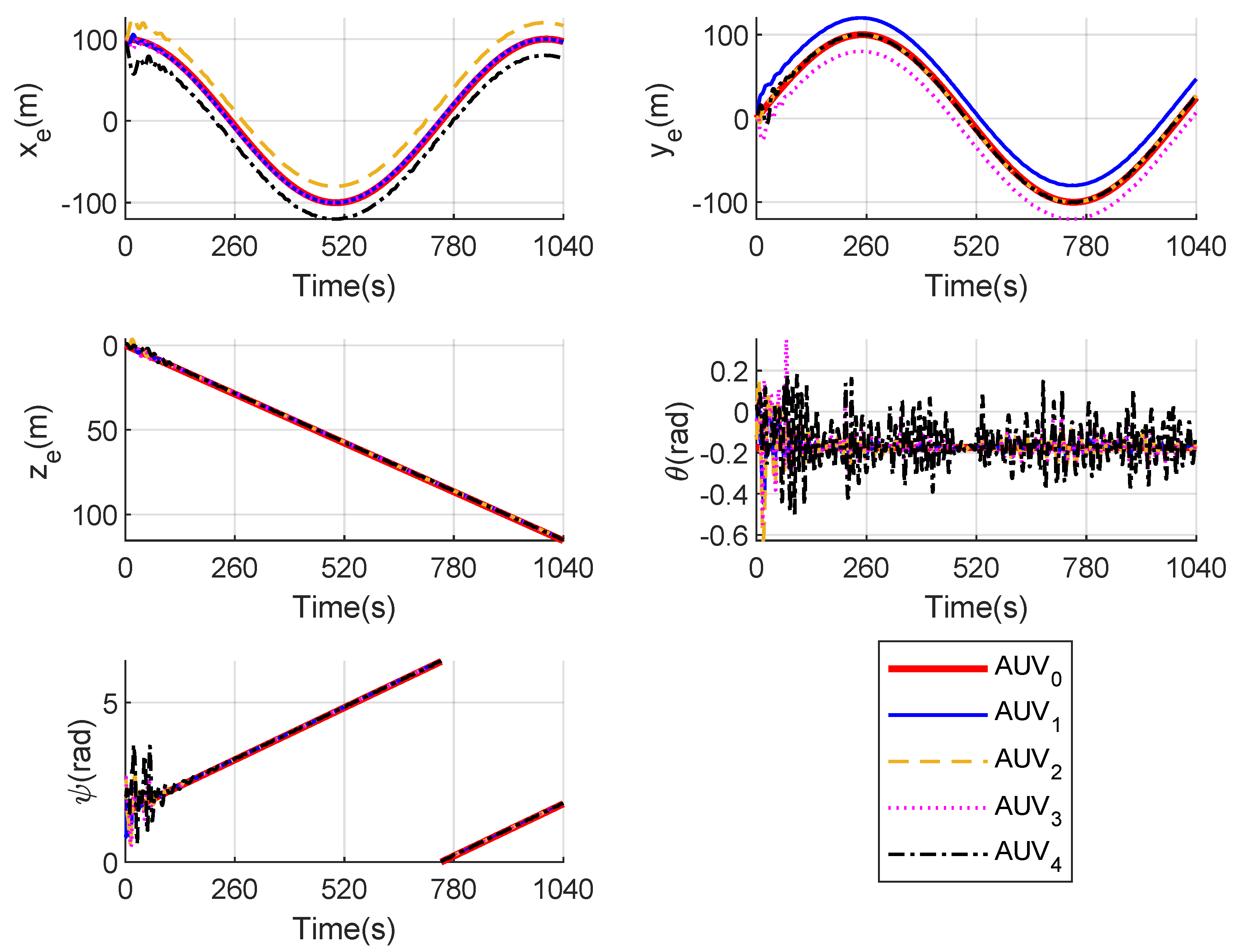
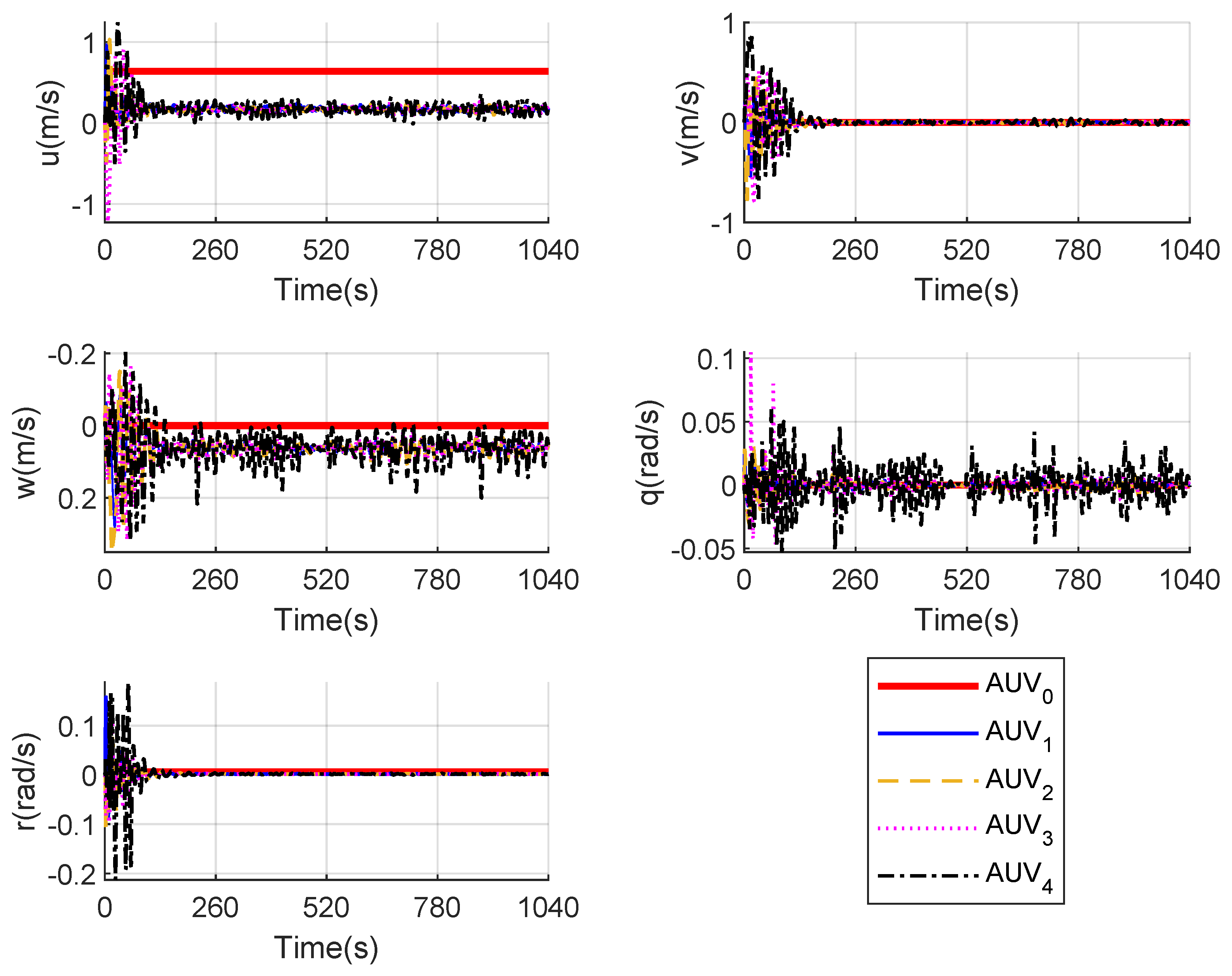
4. Simulation Results and Discussion

In this section, some numerical simulations are presented to illustrate the effectiveness of the above results. In all examples, the multi-AUV system consists of one leader $\mathrm{AU}{\mathrm{V}}_0$ and four followers $\mathrm{AU}{\mathrm{V}}_i,i=1,2,3,4$, and there are two communication topologies $G_B$ and G. The nonlinear parameters of AUV model are presented in Ref. [40].

4.1. Example-1

During the operation of multi-AUV system, if the distance between all the vehicles is relatively close and the communication devices are all intact, each follower can receive the state information of the leader, and the followers can transmit information to each other. Then the system is under the ideal communication topology, which is shown in Figure 2.

Associated with $G_B$ and G in Figure 2, the matrix B and L can be given as

$$B=\left[\begin{array}{cccc}1& 0& 0& 0\\ 0& 1& 0& 0\\ 0& 0& 1& 0\\ 0& 0& 0& 1\end{array}\right],L=\left[\begin{array}{cccc}3& -1& -1& -1\\ -1& 3& -1& -1\\ -1& -1& 3& -1\\ -1& -1& -1& 3\end{array}\right].$$

After calculation, the eigenvalues of matrix $(B+L)$ can be derived as ${\lambda }_1=1$, ${\lambda }_2=5$, ${\lambda }_3=5$, ${\lambda }_4=5$. The parameters in the coordinated controller (9) are selected as $\alpha =0.25$, $\beta =0.92$. And the sampling period $T=0.2$ s. They can all make the three inequalities in Theorem 1 hold.

Based on the above parameters, we first select the random state and verify the stability of the error system (10). The errors of position state and velocity state between the leader and followers are presented in Figure 3 and Figure 4, in the multi-AUV second-order integrator dynamics. Obviously, the errors will eventually converge asymptotically to zero, so the error system (10) is globally asymptotically stable.

Then the two-dimensional coordinated formation simulation for multiple AUVs is performed. The path of leader is expressed as

$$\left\{\begin{array}{ccc}& x_e=10+t,y_e\left(t\right)=10,\hfill & \hfill 0⩽t<100\\ & x_e=110+25sin(\pi -\frac{t-100}{25}),y_e=35+25cos(\pi -\frac{t-100}{25}),\hfill & \hfill 100⩽t<178.4\\ & x_e=110+25sin(\pi +\frac{t-178.4}{25}),y_e=85+25cos(\pi +\frac{t-178.4}{25}),\hfill & \hfill 178.4⩽t<256.8\\ & x_e=110+t,y_e=110,\hfill & \hfill 256.8⩽t<358.8\end{array}\right.$$

Initial locations of followers are randomly distributed in the $[0,10]\times [0,10]$.The position difference between the followers and the leader in the pre-defined formation is $[8;-8]$, $[-8;-8]$, $[8;8]$, $[-8;8]$, respectively.

The simulation results of multiple AUVs formation are illustrated in Figure 5, Figure 6 and Figure 7. The updated information on the position and angle of AUVs, in the earth-fixed coordinate system, are given in Figure 5. Figure 6 shows the velocities of the multi-AUV system with some curves. The formation trajectory of multiple AUVs is depicted in Figure 7, and the desired formation is developed. These indicates that the proposed coordinated controller (9) and the parameters chosen according to Theorem 1 enable the followers to track the leader reliably.

4.2. Example-2

When the vehicles are far apart or communication facilities are damaged in the multi-AUV system, the communication between them will fail and only data can be exchanged with other vehicles. In this case, the system is under alterable communication topology, and we assume it as shown in Figure 8.

The matrix B and L can be given as

$$B=\left[\begin{array}{cccc}1& 0& 0& 0\\ 0& 0& 0& 0\\ 0& 0& 0& 0\\ 0& 0& 0& 0\end{array}\right],L=\left[\begin{array}{cccc}1& -1& 0& 0\\ -1& 1& 0& 0\\ -1& 0& 1& 0\\ 0& 0& -1& 1\end{array}\right].$$

The eigenvalues of matrix $(B+L)$ can be derived as ${\lambda }_1=1$, ${\lambda }_2=1$, ${\lambda }_3=0.382$, ${\lambda }_4=2.618$. The parameters of the controller and sampling period we chose are the same as in Section 4.1, and the inequalities in Theorem 1 also hold.

Figure 9 and Figure 10 illustrate the errors of the position and velocity states in the discrete-time AUV model, respectively. Undoubtedly, system (10) can be stable with alterable communication topology showed in Figure 8. Then we perform the same formation simulation as in Example 1, and the simulation results are showed as Figure 11, Figure 12 and Figure 13. In comparison with Figure 3, Figure 4, Figure 5, Figure 6 and Figure 7, Figure 9, Figure 10, Figure 11, Figure 12 and Figure 13 also verify the effectiveness of the coordinated controller (9) and the availability of the constraint on alterable topology in Theorem 1, but the error convergence is slower, and the time required to form a preset formation is longer. Therefore, the communication topology of a multi-AUV system affects the coordinated control performance to a certain extent.

4.3. Example-3

Due to the slower speed of acoustic transmission, the exchange of information between vehicles suffers a time delay. Then we consider the communication topology with time-varying communication delay of the multi-AUV system as shown in Figure 8. Matrixes B and L have been given in Section 4.2. The parameters in the coordinated controller (17) are selected as $\alpha =0.068$, $\beta =0.272$, and $T=0.2 \mathrm{s}$. The above parameters and all the eigenvalues of matrix $(B+L)$ allow the inequalities in Theorem 2 to hold. The boundaries of d related to the time-varying delay ∂ are set as $d_m=1$, $d_M=4$.

Assume that the three-dimensional path of the leader is represented as

$$x_e=100cos\left(\frac{\pi t}{500}\right),y_e=100sin\left(\frac{\pi t}{500}\right),z_e=0.111t,0<t⩽1040.$$

And the initial locations of followers are randomly distributed in the $[90,100]\times [0,10]\times [0,1]$. The preset position differences between the leader and followers in designed formation are $[0;20;0]$, $[20;0;0]$, $[0;-20;0]$, $[-20;0;0]$, respectively.

As in the previous two examples, we first demonstrate that the error system (18) is asymptotically stable with random initial values. Figure 14 and Figure 15 describe the state errors of the second-order discrete-time model with time-varying time delay. It is clear that the errors all converge asymptotically to zero, indicating that the error system is stable. The three-dimensional formation simulation results with communication delay and alterable topology are presented in Figure 16, Figure 17 and Figure 18. As we can see from these figures, the followers can still effectively track the trajectory of the leader and constitute the desired formation, regardless of the communication delay. Therefore, once the time-varying delay and the controller gains such that the inequalities in Theorem 2 hold, our control strategy can resolve the coordinated formation control problem of multiple AUVs. Compared to the simulation results in Example 2 without communication delay as described in Figure 9, Figure 10, Figure 11, Figure 12 and Figure 13, it is noticeable that the errors in Figure 14 and Figure 15 take longer to converge asymptotically to zero. Furthermore, as illustrated in Figure 16, Figure 17 and Figure 18 although the aforementioned control framework enables multiple AUVs to maintain formation under time-varying delay, the control results are notably worse than the case with no delay.

5. Conclusions

In this paper, the coordinated formation control issue of discrete-time multi-AUV system with alterable communication topology subject to time-varying bounded communication delay has been investigated. The AUV model has been simplified by state feedback linearization and represented as a discrete-time form. Then we designed controllers to solve the problem of coordinated formation under two communication conditions, and obtained the sufficient conditions which assure the formation can be achieved through the stability analysis of the error systems. Finally, numerical examples have been given to validate the main results and show that both the communication topology and the communication delay have obvious effects on coordinated control. As the complexity of ocean missions, AUV motion control can be hampered by many factors, such as model uncertainty, external disturbances, and ocean noise [41]. We will consider the coordinated formation control subject to them for future work.

References

- Yang, H.Z.; Wang, C.F.; Zhang, F.M. A decoupled controller design approach for formation control of autonomous underwater vehicles with time delays. IET Control Theory Appl. 2013, 7, 1950–1958. [Google Scholar] [CrossRef]
- Yang, Y.; Xiao, Y.; Li, T.S. A Survey of Autonomous Underwater Vehicle Formation: Performance, Formation Control, and Communication Capability. IEEE Commun. Surv. Tutor. 2021, 23, 815–841. [Google Scholar] [CrossRef]
- Alam, K.; Ray, T.; Anavatti, S.G. Design Optimization of an Unmanned Underwater Vehicle Using Low- and High-Fidelity Models. IEEE Trans. Syst. Man Cybern. Syst. 2017, 47, 2794–2808. [Google Scholar] [CrossRef]
- Kim, J.; Joe, H.; Yu, S.C.; Lee, J.S.; Kim, M. Time-Delay Controller Design for Position Control of Autonomous Underwater Vehicle Under Disturbances. IEEE Trans. Ind. Electron. 2016, 63, 1052–1061. [Google Scholar] [CrossRef]
- Liu, X.; Zhang, M.; Wang, S. Adaptive region tracking control with prescribed transient performance for autonomous underwater vehicle with thruster fault. Ocean Eng. 2020, 196, 106804. [Google Scholar] [CrossRef]
- Tijjani, A.S.; Chemori, A.; Creuze, V. Robust Adaptive Tracking Control of Underwater Vehicles: Design, Stability Analysis, and Experiments. IEEE-ASME Trans. Mechatron. 2021, 26, 897–907. [Google Scholar] [CrossRef]
- Heshmati-Alamdari, S.; Nikou, A.; Dimarogonas, D.V. Robust Trajectory Tracking Control for Underactuated Autonomous Underwater Vehicles in Uncertain Environments. IEEE Trans. Autom. Sci. Eng. 2021, 18, 1288–1301. [Google Scholar] [CrossRef]
- Zhang, W.; Teng, Y.B.; Wei, S.L.; Xiong, H.H.; Ren, H.L. The robust H-infinity control of UUV with Riccati equation solution interpolation. Ocean Eng. 2018, 156, 252–262. [Google Scholar] [CrossRef]
- Zendehdel, N.; Gholami, M. Robust Self-Adjustable Path-Tracking Control for Autonomous Underwater Vehicle. Int. J. Fuzzy Syst. 2021, 23, 216–227. [Google Scholar] [CrossRef]
- Zhang, Z.C.; Wu, Y.Q. Adaptive Fuzzy Tracking Control of Autonomous Underwater Vehicles With Output Constraints. IEEE Trans. Fuzzy Syst. 2021, 29, 1311–1319. [Google Scholar] [CrossRef]
- Cui, R.X.; Ge, S.S.; How, B.V.E.; Choo, Y.S. Leader-follower formation control of underactuated autonomous underwater vehicles. Ocean Eng. 2010, 37, 1491–1502. [Google Scholar] [CrossRef]
- Qi, X. Adaptive coordinated tracking control of multiple autonomous underwater vehicles. Ocean Eng. 2014, 91, 84–90. [Google Scholar] [CrossRef]
- Zhang, Y.; Wang, X.; Wang, S.; Tian, X. Three-dimensional formation–containment control of underactuated AUVs with heterogeneous uncertain dynamics and system constraints. Ocean Eng. 2021, 238, 109661. [Google Scholar] [CrossRef]
- Wei, H.L.; Shen, C.; Shi, Y. Distributed Lyapunov-Based Model Predictive Formation Tracking Control for Autonomous Underwater Vehicles Subject to Disturbances. IEEE Trans. Syst. Man Cybern. Syst. 2021, 51, 5198–5208. [Google Scholar] [CrossRef]
- Mesbahi, M. On state-dependent dynamic graphs and their controllability properties. IEEE Trans. Autom. Control 2005, 50, 387–392. [Google Scholar] [CrossRef]
- Cao, Y.C.; Yu, W.W.; Ren, W.; Chen, G.R. An Overview of Recent Progress in the Study of Distributed Multi-Agent Coordination. IEEE Trans. Ind. Inf. 2013, 9, 427–438. [Google Scholar] [CrossRef] [Green Version]
- Olfati-Saber, R.; Fax, J.A.; Murray, R.M. Consensus and cooperation in networked multi-agent systems. Proc. IEEE 2007, 95, 215–233. [Google Scholar] [CrossRef] [Green Version]
- Hatano, Y.; Mesbahi, M. Agreement over random networks. IEEE Trans. Ind. Inf. 2005, 50, 1867–1872. [Google Scholar] [CrossRef]
- Huang, M.Y.; Dey, S.; Nair, G.N.; Manton, J.H. Stochastic consensus over noisy networks with Markovian and arbitrary switches. Automatica 2010, 46, 1571–1583. [Google Scholar] [CrossRef] [Green Version]
- Ai, X.D.; Song, S.J.; You, K.Y. Second-order consensus of multi-agent systems under limited interaction ranges. Automatica 2016, 68, 329–333. [Google Scholar] [CrossRef]
- Huang, N.; Duan, Z.S.; Chen, G.R. Some necessary and sufficient conditions for consensus of second-order multi-agent systems with sampled position data. Automatica 2016, 63, 148–155. [Google Scholar] [CrossRef]
- Yang, S.S.; Liao, X.F.; Liu, Y.B. Second-order consensus in directed networks of identical nonlinear dynamics via impulsive control. Neurocomputing 2016, 179, 290–297. [Google Scholar] [CrossRef]
- Dong, X.W.; Yu, B.C.; Shi, Z.Y.; Zhong, Y.S. Time-Varying Formation Control for Unmanned Aerial Vehicles: Theories and Applications. IEEE Trans. Control Syst. 2015, 23, 340–348. [Google Scholar] [CrossRef]
- Kuriki, Y.; Namerikawa, T. Formation Control of UAVs with a Fourth-order Flight Dynamics. In Proceedings of the 2013 IEEE 52nd Annual Conference on Decision and Control (CDC), Firenze, Italy, 10–13 December 2013; pp. 6706–6711. [Google Scholar]
- Kuriki, Y.; Namerikawa, T. Consensus-based Cooperative Formation Control with Collision Avoidance for a Multi-UAV System. In Proceedings of the 2014 American Control Conference (ACC), Portland, OR, USA, 4–6 June 2014; pp. 2077–2082. [Google Scholar]
- Fabiani, F.; Fenucci, D.; Caiti, A. A distributed passivity approach to AUV teams control in cooperating potential games. Ocean Eng. 2018, 157, 152–163. [Google Scholar] [CrossRef]
- Shojaei, K. Neural network formation control of underactuated autonomous underwater vehicles with saturating actuators. Neurocomputing 2016, 194, 372–384. [Google Scholar] [CrossRef]
- Yan, Z.P.; Pan, X.L.; Yang, Z.W.; Yue, L.D. Formation Control of Leader-Following Multi-UUVs With Uncertain Factors and Time-Varying Delays. IEEE Access 2019, 7, 118792–118805. [Google Scholar] [CrossRef]
- Zhang, W.; Zeng, J.; Yan, Z.P.; Wei, S.L.; Tian, W.D. Leader-following consensus of discrete-time multi-AUV recovery system with time-varying delay. Ocean Eng. 2021, 219, 108258. [Google Scholar] [CrossRef]
- Yan, Z.; Zhang, C.; Tian, W.; Zhang, M. Formation trajectory tracking control of discrete-time multi-AUV in a weak communication environment. Ocean Eng. 2022, 245, 110495. [Google Scholar] [CrossRef]
- Ren, W.; Beard, R.W. Consensus seeking in multiagent systems under dynamically changing interaction topologies. IEEE Trans. Autom. Control 2005, 50, 655–661. [Google Scholar] [CrossRef]
- Fossen, T.I. Guidance and Control of Ocean Vehicles; John Wiley & Sons: Chichester, UK, 1994. [Google Scholar]
- Fossen, T.I. Handbook of Marine Craft Hydrodynamics and Motion Control; John Wiley and Sons: Hoboken, NJ, USA, 2011. [Google Scholar]
- Yan, Z.P.; Liu, Y.B.; Zhou, J.J.; Zhang, W.; Wang, L. Consensus of multiple autonomous underwater vehicles with double independent Markovian switching topologies and timevarying delays. Chin. Phys. B 2017, 26, 040203. [Google Scholar] [CrossRef]
- Graham, A. Kronecker Products and Matrix Calculus: With Applications; Courier Dover Publications: Mineola, NY, USA, 1981. [Google Scholar]
- Kovacs, I.; Silver, D.S.; Williams, S.G. Determinants of commuting-block matrices. Am. Math. Mon. 1999, 106, 950–952. [Google Scholar] [CrossRef]
- Ogata, K. Discrete-Time Control Systems, 2nd ed.; Prentice-Hall, Inc.: Hoboken, NJ, USA, 1995. [Google Scholar]
- Huang, L.; Wang, L.; Hollot, C.V. On robust stability of polynomials and related topics. J. Syst. Sci. Complex. 1992, 5, 42–54. [Google Scholar]
- Liu, H.Y.; Xie, G.M.; Wang, L. Necessary and sufficient conditions for solving consensus problems of double-integrator dynamics via sampled control. Int. J. Robust Nonlinear Control 2010, 20, 1706–1722. [Google Scholar] [CrossRef]
- Yan, Z.P.; Yu, H.M.; Li, B.Y. Bottom-following control for an underactuated unmanned undersea vehicle using integral-terminal sliding mode control. J. Cent. South Univ. 2015, 22, 4193–4204. [Google Scholar] [CrossRef]
- Yan, Z.; Xu, D.; Chen, T.; Zhang, W.; Liu, Y. Leader-Follower Formation Control of UUVs with Model Uncertainties, Current Disturbances, and Unstable Communication. Sensors 2018, 18, 662. [Google Scholar] [CrossRef] [Green Version]
Publisher’s Note: MDPI stays neutral with regard to jurisdictional claims in published maps and institutional affiliations. |
© 2022 by the authors. Licensee MDPI, Basel, Switzerland. This article is an open access article distributed under the terms and conditions of the Creative Commons Attribution (CC BY) license (https://creativecommons.org/licenses/by/4.0/).
Share and Cite
Yu, H.; Zeng, Z.; Guo, C. Coordinated Formation Control of Discrete-Time Autonomous Underwater Vehicles under Alterable Communication Topology with Time-Varying Delay. J. Mar. Sci. Eng. 2022, 10, 712. https://0-doi-org.brum.beds.ac.uk/10.3390/jmse10060712
Yu H, Zeng Z, Guo C. Coordinated Formation Control of Discrete-Time Autonomous Underwater Vehicles under Alterable Communication Topology with Time-Varying Delay. Journal of Marine Science and Engineering. 2022; 10(6):712. https://0-doi-org.brum.beds.ac.uk/10.3390/jmse10060712
Chicago/Turabian StyleYu, Haomiao, Zhenfang Zeng, and Chen Guo. 2022. "Coordinated Formation Control of Discrete-Time Autonomous Underwater Vehicles under Alterable Communication Topology with Time-Varying Delay" Journal of Marine Science and Engineering 10, no. 6: 712. https://0-doi-org.brum.beds.ac.uk/10.3390/jmse10060712