Integrated Carbon Emission Estimation Method and Energy Conservation Analysis: The Port of Los Angles Case Study

Abstract

Port environmental problems have gradually become the primary concern of port authorities. The future trend of port carbon emissions is crucial to port authorities and managers in formulating regulations and optimizing operation schedules. Owing to the limitations of current prediction methods and the complex social–environmental impact, the estimation results of port carbon emissions have insufficient accuracy to support port development in the future. In this work, the stochastic impacts by regression on population, affluence, and technology (STIRPAT)–long short-term memory (LSTM)–autoregressive integrated moving average with explanatory variable (ARIMAX) integrated model is proposed for the estimation of the carbon emission of Port of Los Angeles to improve the reliability of emission prediction. Macroeconomic indicators that affect port throughput are selected using the principal component analysis—multiple linear regression model. The chosen indicators are then combined with long-term historical port throughput data as the input of the multivariate autoregressive integrated moving average (ARIMAX) model to predict port throughput. Indicators related to port carbon emissions are verified by the STIRPAT model. The LSTM–ARIMAX integrated model is then applied to estimate the emission tendency, which can be useful in developing corresponding carbon reduction strategies and further understanding port emissions. Results show that the proposed method can significantly improve the estimation accuracy for port emission by 11% compared with existing techniques. Energy conservation strategies are also put forward to assist port authorities in achieving the peak clipping of port carbon emission.

1. Introduction

Environmental issues, including air pollution, noise pollution, low water quality, loss of biodiversity, and destruction of natural habitats, have always been a concern for ports [1]. According to the European Ports Organization (ESPO) Environmental Report in 2019, low air quality remains the top environmental issue for European ports. Various ports are now speeding up the construction of green ports, with more than half dedicated to berth ships to provide shore power. A third of these countries encourage the use of liquefied natural gas (LNG) fuel mainly for trucks (90%) and barges (20%) [2]. Meanwhile, 56% of the ports offer differentiated environmental charges for ships that exceed regulatory standards, particularly those concerned with air emissions, wastes, and climate change. In addition, 71% of ports have been certified as environmentally friendly, and this value has increased by 17% since 2013. Approximately 82% of ports have environmental monitoring programs that mainly focus on pollution. The investment of each port in environmental protection has increased in recent years [3]. To improve the efficiency of these investments, port managers must predict the future trend of port emissions.

Emission reduction and energy efficiency are pillars of IMO’s greenhouse gas (GHG) targets (50% emission reduction in maritime transport by 2050). There is a lot of research on maritime forecasting. Most use traditional forecasting methods, such as linear regression or ARIMA time series, while some studies use deep-learning algorithms to obtain forecasting data. However, most of these studies have focused on emissions from individual vessels or routes; research on port emission forecasting and reduction is fragmented and underdeveloped. Thus, this work aimed to investigate the role of ports in carbon emission mitigation. A systemic approach is adopted to predict the medium- and long-term changes and trends of port carbon emissions. Forecasting this trend for different ports can help the government in designing regulations and prioritizing different port energy conservation budgets from a regional perspective.

The remainder of this paper is outlined as follows. A literature review, including port carbon emission assessment and port carbon emission reduction, is presented in Section 2, followed by an illustration of the proposed method in Section 3. Real data are collected and then used to verify the carbon emission model, as discussed in Section 4. The accuracy of the proposed model and several methods in optimizing port carbon emissions is evaluated through the result analysis in Section 5. Finally, strategies for energy conservation strategies in ports are proposed in Section 6, and the conclusion is provided in Section 7.

2. Literature Review

2.1. Port Carbon Emission Assessment

Ports are important nodes in shipping logistic networks that operate various types of vehicles and cargo-handling equipment. Therefore, these facilities are regarded as concentration areas producing air pollutants and GHG emissions. Given the usual location of ports near highly populated coastal cities, port stakeholders are undoubtedly concerned with health-impacted air pollutants, such as NOx, SOx, particulate matter (PM), volatile organic compounds (VOCs), and carbon monoxide.

Table 1. Summary of port carbon emission assessment.

No	Study	Emissions	Data Resources	Field		Method
				Port	Shipping Routes
1	Rodrigues et al., 2014	CO2	6 ports in UK		√	Origin-destination method
2	Yan et al., 2020	CO2	Ship noon report		√	Random forest regressor
3	Yu et al., 2021	Relative collision risk	10-year collision data in North China, Korean Penisula, and Japan		√	Beyesian spatio-temporal model
4	Poulsen et al., 2018	CO2, Ox, NOx, and PM	Port authorities in Europe and North America	√		Interviews TIC and EV analysis
5	Berechman and Tseng, 2012	NOx, CO2, PM10, SO2, and VOC	Port of Kaohsiung in 2010	√		Bottom-up method
6	Song et al., 2014	CO2, CH4, N2O, PM10, PM2.5, NOx, SOx, CO, and HC	Collected from 6518 ship calls at Yangshan port in 2009		√	Origin-destination method
7	Theodoropoulos et al., 2021	CO2	Collected from a 165,000-DWT tanker		√	FFNN model RNN model
8	Coraddu et al., 2017	CO2	Collected from a Handymax chemical/product tanker		√	White box model Black box model Grey box model
9	Linh et al., 2021	CO2	Vietnamese branch of a worldwide leading shipping company from February 2017 to January 2019 Vessel tracking the Copernicus Marine Environment monitoring service		√	ANN model
10	Panapakidis et al., 2020	CO2	Ro/Pax vessel shipping from Patras–Igoumenitsa–Bari itinerary		√	FFNN model ENN model
11	Rodrigues et al., 2014	CO2	6 ports in UK		√	Origin-destination method
12	Yan et al., 2020	CO2	Ship noon report		√	Random forest regressor

summarizes the recent studies on the port carbon emission assessment.

Current studies on reducing pollution in the maritime field mainly target the carbon emission optimization of shipping routes [4], the carbon emission prediction of single ships [5], and the pollution reduction strategies [6]. In particular, the effect of sailing speed on carbon emissions is analyzed to achieve a balance between carbon emission’s impact and travel time. In recent years, ports have received significant attention because of the increasing pressure to improve environmental credibility [7]. However, there are certain research gaps in developing port carbon emission reduction strategies.

Carbon emission is mainly calculated on two levels: macroscopic and microscopic. Macroscopic calculation uses the carbon emission accounting method from the perspective of conceptual interpretation and microscopic calculation estimates carbon emission according to different emission sources. Nowadays, most of the studies focus on microscopic analysis.

Berechman and Tseng [8] conducted an emission inventory at Kaohsiung Port in Taiwan using a bottom-up methodology to estimate the associated emission costs of ships and trucks that operated in the port in 2010 and found that tankers, containerships, and bulk ships are the major contributors to ship emissions. Song [9] performed a ship emission study of CO₂, methane (CH₄), nitrous oxide (N₂O), PM₁₀, PM_2.5, NOx, SOx, CO, and HC at Shanghai Yangshan Port in China in 2008 to distinguish in-port ship emissions and the associated social costs. Few studies estimate carbon emissions from a macroscopic perspective.

Meanwhile, deep-learning methods have also been introduced into the assessment of carbon emissions from shipping by predicting the fuel consumption or power of ships to obtain future carbon emissions. Theodoropoulos [10] used feed-forward neural network (FFNN) and recurrent neural network (RNN) to predict the propulsion power of ships and showed that the LSTM in the RNN performed best. Coraddu [11] compared three different methods for ship fuel consumption prediction: white box model, black box model, and grey box model. Liu [12] uses an artificial neural network (ANN) model with average speed, sailing time, ship capacity, wind speed, and wind direction as input variables to predict the fuel consumption of ships across the route. The mean absolute percentage error (MAPE) of the model was 5.89% with good prediction results. Panapakidis [13] tested various deep-learning models to predict fuel consumption of passenger ships, and the results showed that ensemble neural networks (ENN) and FFNN had the best prediction results. However, ports have not yet been covered in these deep-learning research; thus, there is a necessity to use deep learning-models to predict carbon emissions from ports.

2.2. Port Carbon Emission Reduction

GHG emission reduction and energy efficiency improvement are important measures for the development of green and sustainable ports. With the expected increase in shipping emissions, the IMO has outlined a guideline for developing an emission reduction plan for ports [1]. This strategy sent a strong signal to ports to reduce shipping GHG emissions at the ship port interface. To advance their goal, the IMO adopted a resolution to encourage cooperation between ports and shipping companies: “Invitation to member states to encourage voluntary cooperation between the port and shipping sectors to contribute to reducing GHG emissions from ships”.

Strategies for reducing port GHG emissions are proposed from different perspectives, such as enhanced routing [14,15], power and fuels [7,16], management and policies [17,18], and supply chain logistics [19,20].

Different countries adopted various strategies for port carbon emission reduction. The New York Port proposed a system of port environmental management and expanded high-speed rail to build green low-carbon ports [21]. Sydney Port in Australia established “the policy of the government action of air” to fully utilize railways instead of high-fuel-consuming highways [22]. Improving shipping safety by capturing the behavior characteristics of vessels is another solution to reduce port emissions [23,24].

According to the above, only a few quantitative studies have focused on the assessment, forecast, and reduction in carbon emissions at seaports. In the present research, a systematic approach is adopted by combining historical data-based forecasting and strategical, operational optimization methods to address carbon emission issues in container ports.

3. Methodology

This study proposes a new combined model, i.e., the stochastic impacts by regression on population, affluence, and technology (STIRPAT)–long short-term memory (LSTM)–autoregressive integrated moving average with explanatory variable (ARIMAX) integrated model, to predict the future trends of port carbon emissions. In this model, the future traffic demand of the port is obtained by predicting the port throughput, which is then used to predict the overall port carbon emissions.

3.1. LSTM and STIRPAT

LSTM is an innovative neural network developed based on the recurrent neural network, which produces promising results on a variety of tasks, including language model [25] and speech recognition [26]. Ehrlich et al. [27] constructed an IPAT model to evaluate the effect of population, affluence, and technological factors on the environment. The Kaya equation reformulated IPAT identity, the basis for calculating GHG emissions [28]. Other similar models include ImPACT [29], ImPACTS, and IPBAT [30]. York et al. [31] proposed the STIRPAT model based on the IPAT model and believed that any factor impacting the environment could be introduced into the model. STIRPAT is expressed as follows:

$$I=a{P}^b{A}^c{T}^{d}e$$

(1)

where I, P, A, and T are environmental pressure, population size, affluence, and technology, respectively; a is the coefficient of the model; b, c, and d are the driving indexes; and e is the random error disturbance of the model. According to the STIRAP model, the three main driving factors affecting environmental pollution are population (P), economy (A), and technology (T). Therefore, these three driving factors can also be selected as the impact factors of port carbon emissions. Port throughput corresponds to P, port profit corresponds to A, and carbon emission intensity corresponds to T. Given their strong correlation, port profit can be combined with port throughput. Finally, port throughput and carbon emission density are selected, and their new formulas are as follows:

$$Q=a{P}^b{T}^{c}e$$

(2)

$$\mathit{ln}\left(Q\right)=\mathit{ln}\left(a\right)+b\left(lnP\right)+c\left(lnT\right)+\mathit{ln}\left(e\right)$$

(3)

where Q is the CO₂ emission of the transportation sector, a is a constant, P is the port throughput, T is the carbon emission density used to represent the level of economic development, ε is a random disturbance term, and b and c are elasticity coefficients.

3.2. ARIMA and ARIMAX Model

The ARIMA model is a differentially integrated, moving-average, autoregressive model, one of the methods of time-series-forecasting analysis. In ARIMA(p, d, q), AR is the ‘autoregressive’, p is the number of autoregressive terms; MA is the ‘sliding average’, q is the number of sliding average terms, and d is the number of differences made to make it a smooth series.

The ARIMAX model is an improved version of the ARIMA model and assumes the stability of the output sequence (i.e., dependent variable sequence $\left\{Y_t\right\}$) and input variable sequence (i.e., independent variable sequence)$\left\{X_{1t}\right\},\left\{X_{2t}\right\},\dots ,\left\{X_{kt}\right\}$. The ARIMA model is used to provide the correlation information in the residual sequence $\left\{{\epsilon }_t\right\}$, and the final model is as follows:

$$\left\{\begin{array}{c}{Y}_t=\mu +{\displaystyle {\displaystyle \sum }_{i=1}^k}\frac{{\theta }_i\left(B\right)}{{\phi }_i\left(B\right)}{B}^{li}{X}_{it}+{\epsilon }_t\\ {\epsilon }_t=\frac{\theta \left(B\right)}{\phi \left(B\right)}{a}_t\end{array}\right.$$

(4)

The final model is called the dynamic regression model abbreviated as ARIMAX in which $\phi \left(B\right)$ is the autoregression coefficient polynomial for the residual sequence, $\theta \left(B\right)$ is the moving-average coefficient polynomial for the residual sequence, and $a_t$ is the zero-mean white noise sequence [32].

3.3. PCA–MLR

Principal component analysis (PCA) is a statistical method for rotating and transforming data. It is done by performing a basis transformation in linear space such that the variance of the transformed data projection on a new set of axes is maximized. The axes that have very little variance after the transformation are removed, and the remaining new axes are called principal components, which represent the properties of the original data as closely as possible in a lower dimensional subspace. Multiple linear regression (MLR) is a statistical technique that uses several explanatory variables to predict the outcome of a response variable. The goal of multiple linear regression is to model the linear relationship between the explanatory (independent) variables and the response (causal) variables. Essentially, multiple regression is an extension of ordinary least squares (OLS) regression in that it involves more than one explanatory variable. In fact, a phenomenon is often linked to more than one factor with the optimal combination of multiple independent variables coming together to predict or estimate the dependent variable.

PCA–MLR is a combined model that includes both PCA and MLR. When faced with many observations, using these variables directly as input to the MLR can create uncertainty and sometimes even cause model errors. Therefore, PCA is applied to extract the principal components, and these are fed into the MLR before regression analysis is carried out. This reduces the complexity of the model but also retains the characteristics of the original data.

3.4. Proposed Method

The proposed model consists of four steps. First, the macroeconomic indicators affecting port throughput are selected by principal component analysis (PCA)–multiple linear regression (MLR). Second, the component indicators and historical port throughput data are inputted into the ARIMAX model to predict port throughput. Third, indicators related to port carbon emissions are selected by the STIRPAT model. Finally, the LSTM–ARIMA combined model is used to predict the overall carbon emissions of the port. The flowchart of the proposed model is shown in Figure 1.

4. Empirical Analysis

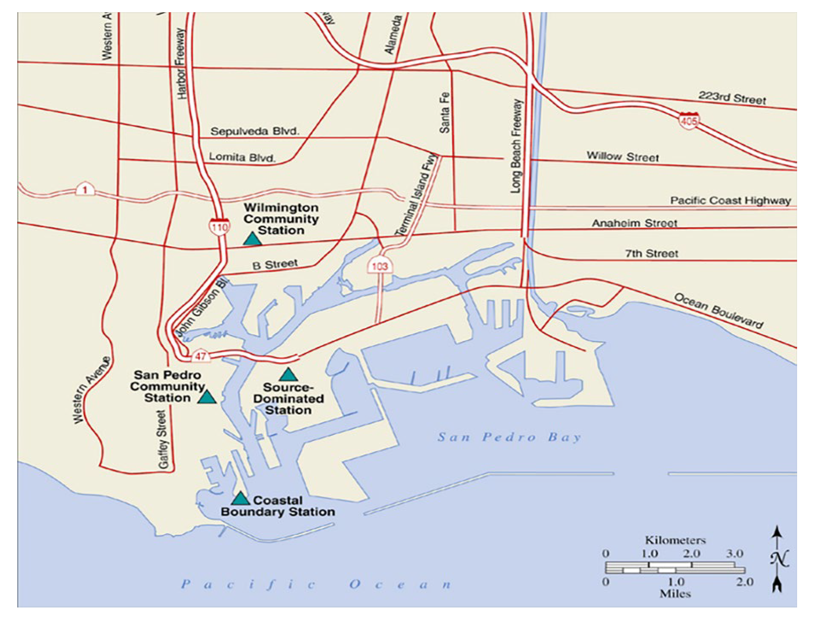
4.1. Introduction of Port of Los Angeles

The Port of Los Angeles is the USA’s premier gateway for international commerce and the busiest seaport in the Western Hemisphere. According to the Port of Los Angeles business report, this facility ranked as the 17th busiest container port globally and 1st in North America, with total handled traffic of 9.34 million twenty-foot equivalent units in 2019. This port is composed of three container terminals, namely, San Pedro, Wilmington, and Terminal Island, which account for approximately 40% of the West Coast’s market share and 17% of the nation’s market share. The major trading countries of the Port of Los Angeles are Pan Pacific countries, mainly East Asia and Southeast Asia. For example, Asian countries represented by China and Japan have significant impacts on the Port of Los Angeles’s throughput, accounting for approximately 20% of the total trade volume. Hence, the indicator selection process before throughout estimation shall consider the economic and trade impact.

4.2. Economic Indicator Selection

From a geographical perspective, the USA, Canada, and Mexico belong to North America. Los Angeles is located on the southwest coast of the USA close to the major ports on the west coast of North America, such as Prince Rupert in Canada and Manzanillo in Mexico.

From an economic perspective, the USA has close trade relationships with Canada and Mexico. As shown in Figure 2, Mexico and Canada are the second and third largest trade partners of the United States, accounting for 14.77% and 14.83%, respectively. China and Japan ranked third and fourth, respectively.

Both perspectives significantly influence today’s modern ports. Such exogenous indicators should be encompassed for the ports, particularly those with throughputs primarily related to import/export amounts and international trade. These variables usually include the domestic, regional, and sometimes even global GDP, import/export amounts, exchange rates, and purchasing power [33,34].

Therefore, the three macroeconomic indicators (

Table 2. Addressed economic indicators.

Macroeconomic Indicator	Short Meaning
GDP	Gross domestic product
Import (billions $)	Goods/services carried into one state from another state
Export (billions $)	Goods manufactured in one state transported to another state

) are exhibited; meanwhile typical countries in North America (NA) and Asia are selected, as shown in

Table 3. Addressed country and region.

Region	Country
NA	U.S., Canada, Mexico
ASIA	China, Japan, Korea

.

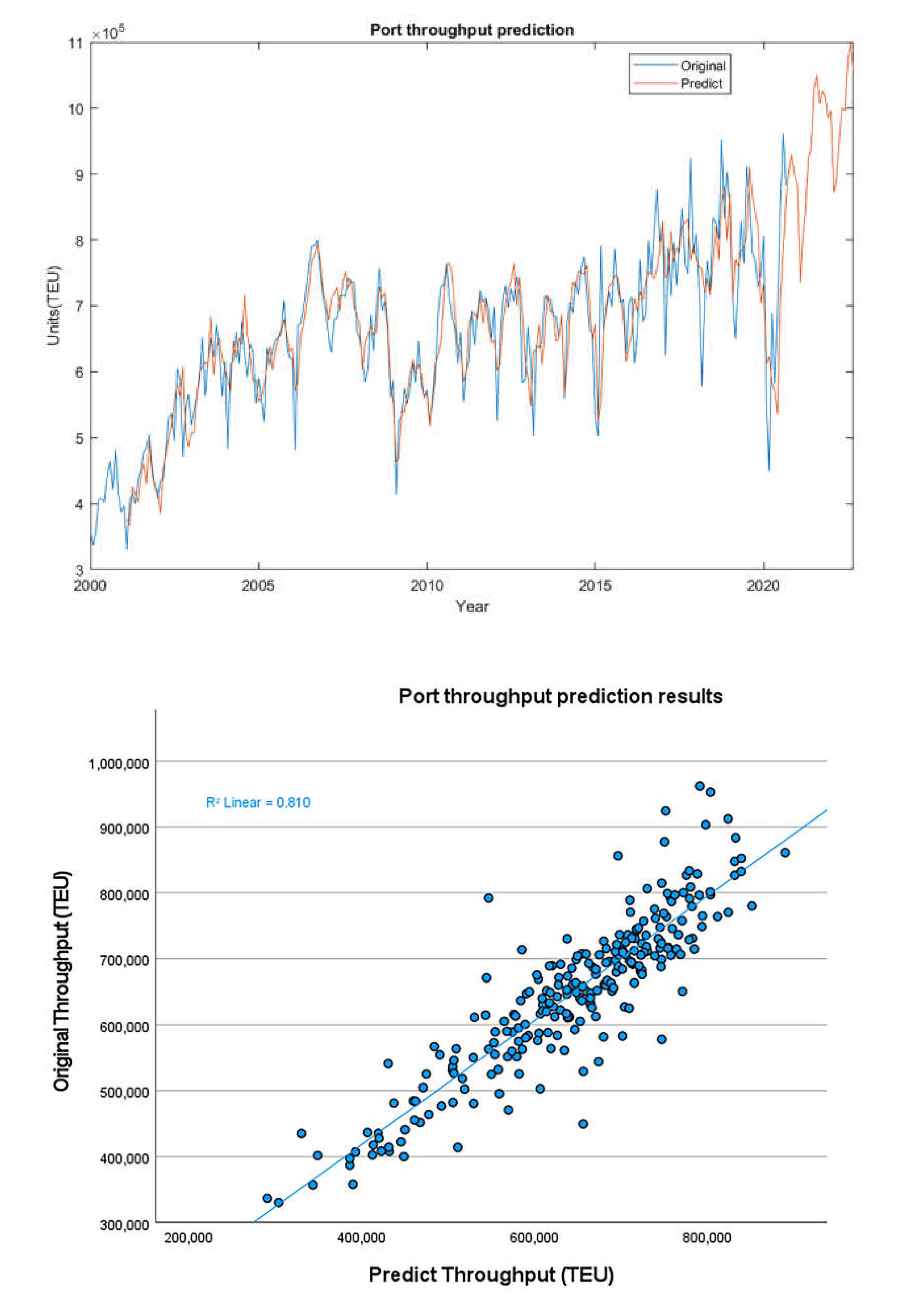
4.3. Port Throughput Forecast

PCA–MLR (principal component analysis–multiple linear regression) is a combination model that can simplify the complexity of the forecast-modeling process. Specifically, PCA reduces the dimensionality of the dataset consisting of many interrelated variables, while retaining as much as possible of the variation present in the dataset. MLR can estimate throughput by using selected variables and historical dataset. Macroeconomic indicators from Section 4.2 are used to predict the throughput. The dimensions of 18 macroeconomic indicators of the six countries must first be reduced by PCA to minimize the interference between these indicators and simplify the whole prediction model.

Prior to PCA, KMO and Bartlett sphericity tests are performed to determine the validity of the data. Dimensionless processing is conducted on the sample data, and the results are shown in

Table 4. KMO and Bartlett’s Test.

KMO and Bartlett’s Test
Kaiser-Meyer-Olkin Measure of Sampling Adequacy.		0.941
Bartlett’s Test of Sphericity	Approx. Chi-square	17,594.292
	df	231.000
	Sig.	0.000

. The KMO measure value is 0.941, and the significance rate of the Bartlett spherical test chi-square statistic is less than 0.010. Therefore, the sample data are suitable for PCA.

PCA is conducted on the dimensionless data for variance analysis. Figure 3 (Factor Scree Plot) shows that the cumulative contribution rate of the principal component reaches 89.1%. Therefore, the components can be attributed to a single factor. The United States has the largest economy in the world, and its major importers and neighboring countries are deeply affected by its economic trends. Consequently, even a single factor can be used to explain the overall situation of the imports and exports of the port.

The linear regression results of the new factor and port throughput data are shown in

Table 5. Coefficients of Linear Regression ^a.

Model	Unstandardized Coefficients		Standardized Coefficients	t	Sig.
	B	Std. Error	Beta
(Constant)	647618.5	5211.9		124.258	0.000
REGR factor score	90915.38	5222.397	0.742	17.409	0.000

^a Dependent Variable: Port.

. The extracted factor has no collinearity with each other, and their significance is less than 0.05. Therefore, the new factor has an impact on port throughput.

As shown in Figure 4, the economic factor and port throughput data are inputted into the ARIMAX model for prediction. The model shows a good overall prediction effect, and the high fitting degree between the model and the actual throughput value can accurately reflect the monthly change trend of port throughput. The R and mean absolute percentage error (MAPE) values of the whole model are 0.81 and 6.149, respectively, implying that the ARMIAX model has a relatively small prediction error and relatively high prediction accuracy. The fitted results demonstrate that the proposed framework is reliable on the prediction of port throughput. The port industry has been severely hit, causing the social and economic-related data to be dramatic changed. And some evidence proved that the complexity of the tariff barriers leads to inconsistencies between changes in economic indicators and trends in port throughput [35]. It is worth noting that the proposed method is able to obtain a similar trend even under uncertain events, i.e., the sudden decrease in late 2019 to early 2020 compared to the real data. It is mainly because the impact of COVID-19 on countries’ cargo trade, but the influence can be explored in their economic indicators in the future.

4.4. Carbon Emission Factor Selection

Port carbon emissions are normally generated from trucks, yard tractors, gantry cranes, and quay cranes [6,36]. These kinds of equipment are generally operated by diesel engines that usually cause heavy-carbon emissions. Excluding the above mentioned, the activities in port water would also emit much carbon emission with vessel berthing or in/out port activity [37,38,39]. However, this research focuses on the total carbon emission estimation and will not specify the detailed carbon contribution referring to all activities in the port.

The Port of Los Angeles has started monitoring air quality within its operational region of influence in the Los Angeles port since 2005. Figure 5 shows that the monitoring program consists of four air-monitoring stations. As collected in the monitoring data, the monthly average concentration of elemental carbon is directly monitored by four different monitoring sites, including Wilmington community site, Coastal boundary site, San Pedro community site, and Source-dominated site. They can be obtained directly from the station’s monitoring database. Additionally, these data also represent the concentration of CO₂ around the Port of Los Angeles. The obtained carbon emission data includes all activities in the port, including port ground emissions, berthing ships, and ship maneuvers in the port water area. According to the STIRPAT model, the three factors influencing the carbon emissions in the transportation area are as follows: the influence of traffic itself, economic development, and technology [40]. Accordingly, port throughput directly affects the amount of traffic carbon emissions and therefore, could be considered as the first indicator. The second factor is port revenue that can directly reflect economic development and is closely related to port throughput. Further, carbon emission intensity is an indicator that can evaluate port emission efficiency level, which is calculated by Equation (5). Lower emission intensity means less CO₂ is produced per unit of energy consumption. It also implies that the target port applied emerging environmental purification technology, for example, using fossil-free energy or improving energy efficiency in ways to minimize the proportion of non-green energy consumption. In the STIRPAT model, carbon intensity is as a technology measure indicator to illustrate the green level of technologies and the changing of port emission. In addition, the carbon intensity is also an influential factor to impact the final results of port emission in Equation (2). In Equation (5), the total consumed fossil and total carbon emission are obtained by the California transportation sector. The descriptive statistics for all data are shown in Table 6. There are no extreme values, and all descriptive statistics are normal.

$$E{i}_{CO2}=\frac{E_{CO2}}{C{E}_{CO2}}$$

(5)

• $Ei$: CO₂ emission intensity (btu/kg)
• $E_{CO2}$: CO₂ emission (kg)
• $C{E}_{CO2}$: Consumed energy (btu)

Figure 5. Locations of four monitoring stations (colored triangles).

Figure 5. Locations of four monitoring stations (colored triangles).

Table 6. Descriptive statistics of carbon emission factors.

Descriptive Statistics	Range	Minimum	Maximum	Mean		Std. Deviation	Variance
	Statistic	Statistic	Statistic	Statistic	Std. Error	Statistic	Statistic
EC	3.370	0.140	3.510	0.891	0.053	0.726	0.527
Emission Intensity	3.552	66.838	70.390	68.238	0.077	1.058	1.119
TEU	547,922.450	413,910.300	961,832.750	690,449.291	6868.992	93,932.049	8.82 × 109

Table 6. Descriptive statistics of carbon emission factors.

Descriptive Statistics	Range	Minimum	Maximum	Mean		Std. Deviation	Variance
	Statistic	Statistic	Statistic	Statistic	Std. Error	Statistic	Statistic
EC	3.370	0.140	3.510	0.891	0.053	0.726	0.527
Emission Intensity	3.552	66.838	70.390	68.238	0.077	1.058	1.119
TEU	547,922.450	413,910.300	961,832.750	690,449.291	6868.992	93,932.049	8.82 × 109

4.5. Carbon Emission Forecast

The emission forecast includes three steps. First, the historical carbon emission, port throughput, and port carbon emission intensity are inputted into the STIRPAT model. The residuals obtained by STRIPAT are then loaded onto the LSTM model to update the prediction residual values and simulate the real situation. The above results are added to the linear part of values in the LSTM–ARIMAX model to obtain the final emission, and the final values are shown in Figure 6. Forecast results for port carbon emissions revealed a fluctuating tendency, changing the same as the original emission. The “original” in the figure represents the real emission data.

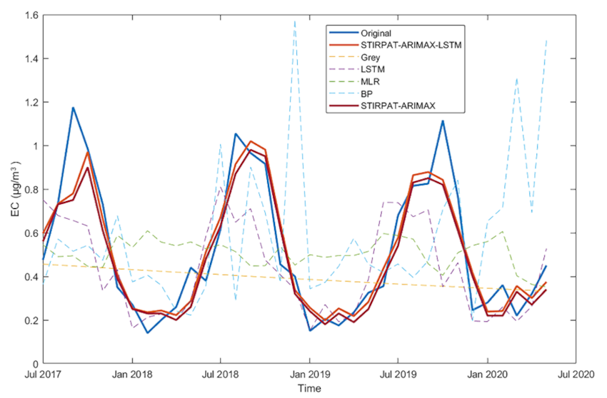
4.6. Accuracy Assessment

To date, no method has been developed for directly evaluating the prediction accuracy. In general, several performance indicators are simultaneously employed to examine the model results. A comprehensive evaluation of performance indicators helps to understand the advantages and disadvantages of the prediction methods. In this work, MAPE, root mean square error (RMSE), and mean direction accuracy (MDA) are used to evaluate the prediction effect. Their formulas are as follows:

$$\mathrm{MAPE}=100\frac{1}{N}{\displaystyle \sum }_{i=1}^N\left|\frac{{\widehat{y}}_i-y_i}{y_i}\right|$$

(6)

$$\mathrm{RMSE}=\sqrt{\frac{1}{N}{\displaystyle \sum }_{i=1}^N{\left({\widehat{y}}_i-y_i\right)}^2}$$

(7)

$$\mathrm{MDA}=\frac{1}{n}{\displaystyle \sum }_{i=1}^n{a}_t,a_t=\left\{\begin{array}{c}1 \mathrm{i}\mathrm{f} \left({\widehat{y}}_i-{\widehat{y}}_{i-1}\right)\left(y_t-y_{t-1}\right)\ge 0\\ 0 otherwise\end{array}\right.$$

(8)

where $y_i$ and ${\widehat{y}}_i$ are the actual and predicted values, respectively. MAPE and RMSE are used to evaluate the numerical accuracy of models, and MDA is applied to examine the accuracy of model trends. Small MAPE and RMSE values indicate good model prediction. Within the MDA range of 0–1, a value closer to 1 also implies good model prediction.

5. Result Analysis

The STIRPAT–LSTM–ARIMAX model is integrated to estimate the carbon emissions of the Port of Los Angeles. The results of the five models are compared to verify the prediction performance of the proposed model, as shown in Figure 7. The prediction performance assessments of the seven models are listed in

Table 7. Estimation performance of port carbon emission models.

Model Name	RMSE	MAPE	MDA	RMSE Diff	MAPE Diff
STIRPAT–ARIMAX–LSTM	0.0145	7.9306	0.685	/	/
STIRPAT–ARIMAX	0.0161	7.9421	0.629	11.08%	0.15%
ARIMA	0.0163	8.9149	0.571	12.58%	12.41%
MLR	0.1084	26.3284	0.429	648.40%	231.99%
BP	0.1901	29.6243	0.486	1213.20%	273.55%
Gray	0.1059	17.7568	0.429	631.15%	123.90%
LSTM	0.0597	10.5881	0.629	271.45%	33.32%

. The second to fourth column in Table 7 shows the numerical results for the different methods of verification.

An obvious discrepancy is noticed in the fifth and sixth columns among the different methods. The references for these values are RMSE and MAPE. It implies that the proposed integrated model has a significant improvement compared to the other classical prediction models, excluding the STIRPAT–ARIMAX combined model, which can be regarded as part of the proposed method.

In Table 7, the MDA value of STIRPAT–ARIMAX is slightly larger than that of STIRPAT–ARIMAX–LSTM. The RMSE of STIRPAT–ARIMAX–LSTM is reduced by 11.08%, and its MDA is improved by 8.33%. The combination of STIRPAT and ARIMAX–LSTM can yield the best prediction results (MAPE = 7.9306%, RMSE = 0.0145, MDA = 24). Those findings proved that the proposed model exhibits the highest accuracy of the estimation performance than the selected classical prediction models.

6. Energy Conservation Strategies in Port

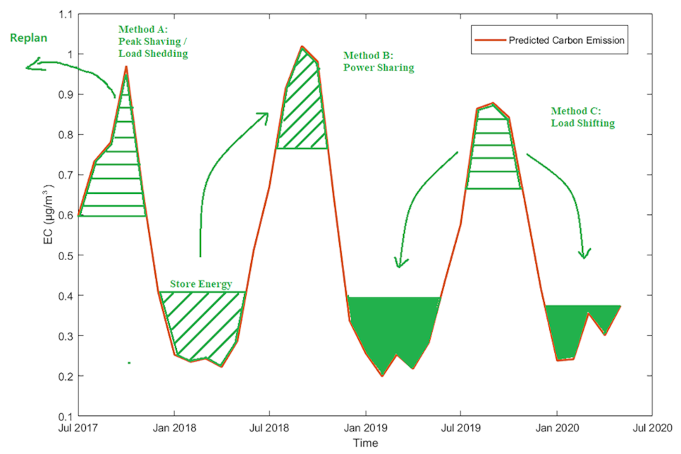
6.1. Peak Shaving, Load Shifting, and Power Sharing

As electrification becomes popular in industry, the number of new port equipment with the use of electricity as their main energy source has been increasing in the past five years [41]. Cargo-handling equipment at the Port of Los Angeles is a major contributor of fossil-energy consumption. Therefore, new port equipment has been used in the Port of Los Angeles, including electric cranes, diesel-electric hybrid rubber-tired gantry cranes, and shore power installation at berth to reduce the traditional fossil emissions. However, the carbon emissions still maintain a similar peak level as does the throughput increase according to the results in Figure 4 and Figure 6. Therefore, the port authority in the Port of Los Angeles should not increase the investment on electrification in a disorderly manner to avoid imbalance between investment and carbon emissions.

Peak shaving, load shifting, and power sharing are innovative operations in port management. Combining the estimation results of the Port of Los Angeles with those innovative strategies can effectively reduce the port’s carbon emissions. Additionally, it is necessary to propose a different energy conservation policy in referring to the rolling characteristic of carbon emissions.

In this research, the carbon emission estimation results imply that port activities and energy consumption have a strong connection with each other and are cyclical and fluctuating, which validate findings that there exists Granger causality between energy consumption and emissions [42,43,44]. Usually, energy consumption in ports can be divided into fixed consumption and floating consumption. When cargo-handling demand is at a low level below fixed consumption, excess emissions are generated; on the contrary, additional costs are inevitably due to the energy gap. Hence, energy conservation strategies, for example, peak-shaving strategies, can be used to mitigate the imbalance between fixed consumption and floating consumption by using the proposed integrated estimation method to capture the emission cycle feature and then achieve the objectives of improving energy efficiency and reducing carbon emission.

Three energy conservation strategies are suggested in the management of the Port of Los Angeles: (1) peak shaving (load shedding), which is shutting down non-critical loads during peak months or time intervals; (2) load shifting, which is shifting of energy demand to off-peak periods during peak periods [45]; (3) power sharing, which is using any stored energy for the peak demand of energy.

Less energy consumption means less carbon emissions. Based on the Port of Los Angeles emission result, Figure 8 illustrates how the energy can be allocated efficiently.

(1)

The port authority shall distinguish which non-critical energy loads can be optimized or even shut down from existing plans by using the peak-shaving method. Geerlings [46] pointed out that quay cranes (QCs) (i.e., ship-to-shore cranes) are one of the largest consumers of electricity in the port. Thus, limiting the number of simultaneous QC lifts can significantly reduce peak power demand and have less impact on working hours in the Port of Los Angeles. For example, the peak power consumption drops by 11.1% if one of six QCs is shut down. At the same time, the handling time will increase by 0.03%, and the waiting time per container will increase by 5.5 s. Using less handling equipment and running smoothly during peak hours would help reduce the peak energy consumption. For six QCs as one group, peak demand can be reduced by 19.8% when the maximum allowable electricity demand is set to 12 mw. At the same time, the average waiting time per container only increases by 3.4 s. There are 83 ship-to-shore container cranes in the Port of Los Angeles according to the statistical results from April 2022. Thus, the dynamic optimization of the maximum QCs in each work unit and adjusting the electricity demand are significant for port authorities in every loading/unloading mission of QC allocation.

(2)

It is possible to reschedule the berth activities by load shifting. As the second crest in October 2018 shows in Figure 8, gradually adjusting the activity schedule towards the troughs on both sides can reduce the imbalance between peak and low values. Van [44] showed that the load-shifting method reduced the peak freezer energy consumption by 62.8% on average by using a port refrigerated warehouse as an example of intermittent allocation of power between batches of cold storage. Therefore, the peaking method can also help reduce congestion in different areas of the port. For instance, energy efficiency can be improved during off-peak hours by encouraging reservation systems and truck arrivals in gate operations by using load shifting. Some evidence proved that the load-shifting method reduced the average peak load by 23.1% according to the build dual objectives functions with peak energy and minimum energy demand [47].

(3)

Energy peaks can be regulated by adding energy storage devices integrated with the peak-shaving and load-shifting methods. In addition, if there still exists an energy gap, the excess power in the trough can be stored, and the energy can be shared in the next peak by super-capacitors. For example, load shifting is used first to reduce peak energy demand by 42.8%. Then, the stored energy will be used during peak hours with a further 55% reduction in peak energy demand [43].

Figure 8. Energy conservation strategies of the Port of Los Angeles.

Figure 8. Energy conservation strategies of the Port of Los Angeles.

6.2. Other Effevtive Strategies

The other effective ways for carbon emission reduction can be concluded as four suggestions. First, it is necessary to replace high energy-consuming equipment in the Port of Los Angeles. The replacement methods of high energy-consuming equipment include rubber-tired gantry crane (RTG) oil to electricity, yard truck (YT) oil to gas, and shore power facilities for ships. Since 2014, the port authority has started to convert minority port facilities into the electric drive to improve energy efficiency (See

Table 8. Yard truck exhaust gas emission comparison among different energy sources.

Energy Source	Exhaust Gas Emission
	CO (%)	HC (%)	$\mathbf{N}{\mathbf{O}}_{\mathbf{x}} (\%)$	Fine Particulate Matter (%)	PbO (%)	Toxic Substance (%)
Gasoline (no exhaust gas treatment)	100	100	100	100	100	100
Gasoline (exhaust gas treatment)	25–30	10	25	/	/	50
Diesel	10	10	50–80	100	/	50
Diesel-natural gas	8–10	8–10	50–70	20–40	/	3–10
LPG	10–20	50–70	20–40	/	/	3–10
LNG	0–1	1–3	10–20	/	/	3–10

).

However, most RTGs in ports still use diesel generator sets and are intermittently operated. Given that this equipment must be kept in standby mode, empty consumption will take up most of the time. The actual efficiency of energy conservation is low, but the cost is relatively high. This phenomenon seriously affects the economic benefits for port operators. Moreover, the diesel engine is a double-edged sword that provides strong power but produces serious environmental pollution including gas, noise, and liquid waste.

YT is the vital part of the whole operation loop from berth to storage yard, and the most its engine still uses diesel. A comparison of exhaust gas emission among different energy sources is given in Gupta [48]. The emission of LNG YT per 100 km is approximately 85% lower than that of diesel YT.

Secondly, when combining the peak-shaving, load-shifting, and power-sharing methods, it is necessary to optimize the production process in port management systems. According to the estimated results, the carbon emissions of ports are cyclical and unbalanced, leading to a number of idle equipment during the idle port period. Accurate forecast data can allow ports to adjust the amount of equipment running in each port area in real time following the principle of the peak shaving. However, the waiting queues of vessels for berthing are prolonged when the efficiency of berth operations decreases because of the lack of crane workers. The quantitative evaluation is discussed in Section 6.1. Additionally, this situation raises a new dilemma on how to balance work efficiency and vessel operation requirements.

Next, converting most of the port’s electricity supply to clean energy sources, such as solar, tidal, and wind power, is a direct and effective way to reduce carbon emissions [49]. In addition to external power grids, clean energy power plants can be built to increase the internal power supply ratio. Plans for clean power plants can be based on the forecast of future carbon emissions of the port.

At last, reducing emissions from ships in the port is also a good option [50,51]. Finding clean fuels and integrating renewable energy into the ship’s power system will significantly reduce ship emissions, especially by electrification of ships, which can reduce carbon emissions by up to 51%.

7. Conclusions

In this research, the carbon emissions of the Port of Los Angeles are estimated by using the proposed innovative framework of the integrated STIRPAT–LSTM–ARIMAX model. The accuracy of carbon emission forecast results has significantly improved upon the other single or combined classical models, and multi-demission influencing indicators are identified.

The results indicate that (1) the prediction results of carbon emission are more reliable and more accurate by over 11% than the others. In detail, the integrated model shows better performance than the other six classical forecast models that refer to the evaluation indictors, RSME, MAPE, and MDA. (2) Carbon emissions of LA PORT have a strong correlation with throughput that would easily be affected by Asian countries, i.e., the tariff barriers between the U.S. and China from 2018. Other proof can be found from 2020 when the prediction curve began to drop sharply during the same time the COVID-19 epidemic spread around the world. (3) Port throughput, port revenue, and carbon emission efficiency are identified to be the most influential indictors during the carbon emission prediction stage, and (4) the proposed framework is progressive and has potential implementation outside of the Port of Los Angeles.

According to the above results, energy conservation strategies for port authorities are accordingly given, including (1) combination of peak-shaving, load-shifting, and power-sharing strategies with the characteristics of carbon emission results, i.e., using stored energy in the case of peak energy demand periods or shifting the energy demand in the peak period to non-peak periods; (2) investment on green port infrastructures should be linked to changing trends in carbon emissions; (3) replacing high-energy-consuming equipment, i.e., yard truck oil to gas and shore power facilities for ships; (4) improving and optimizing the efficiency of port operations to avoid unnecessary waste of resources and unacceptable queue lengths at anchor in port waters; and (5) upgrading of berthing vessel engines to enhance flexibility and the economy of the green port program.

The proposed method has some limitations. For example, the impact of the atmospheric environment surrounding the target port and the attrition caused by the COVID-19 epidemic must be further discussed. In future research, the micro-driven factors related to carbon emissions will be further explored. Another limitation is that the proposed method is more suitable for medium and large ports, which have good data collection systems. The ports have good data management systems, can collect a variety of information, and historical data is well maintained, thus providing sufficient training sets for the models. In addition, the model is mainly used to predict carbon emissions for the port as a whole, and further research is needed for carbon emissions at the micro level of the port (e.g., individual ships, trucks, etc.).

References

1. International Maritime Organization. Fourth IMO Greenhouse Gas Study 2020; International Maritime Organization (IMO): London, UK, 2020. [Google Scholar]
2. European Ports Organization. ESPO Environmental Report 2019; EcoPortsinSights: Brussel, Belgium, 2019. [Google Scholar]
3. Bellou, N.; Gambardella, C.; Karantzalos, K.; Monteiro, J.G.; Canning-Clode, J.; Kemna, S.; Arrieta-Giron, C.A.; Lemmen, C. Global assessment of innovative solutions to tackle marine litter. Nat. Sustain. 2021, 4, 516–524. [Google Scholar] [CrossRef]
4. Rodrigues, V.S.; Beresford, A.; Pettit, S.; Bhattacharya, S.; Harris, I. Assessing the cost and CO2e impacts of rerouteing UK import containers. Transp. Res. Part A Policy Pract. 2014, 61, 53–67. [Google Scholar] [CrossRef]
5. Yan, R.; Wang, S.; Du, Y. Development of a two-stage ship fuel consumption prediction and reduction model for a dry bulk ship. Transp. Res. Part E Logist. Transp. Rev. 2020, 138, 101930. [Google Scholar] [CrossRef]
6. Yu, Y.; Sun, R.; Sun, Y.; Wu, J.; Zhu, W. China’s Port Carbon Emission Reduction: A Study of Emission-Driven Factors. Atmosphere 2022, 13, 550. [Google Scholar] [CrossRef]
7. Poulsen, R.T.; Ponte, S.; Sornn-Friese, H. Environmental upgrading in global value chains: The potential and limitations of ports in the greening of maritime transport. Geoforum 2018, 89, 83–95. [Google Scholar] [CrossRef] [Green Version]
8. Berechman, J.; Tseng, P.-H. Estimating the environmental costs of port related emissions: The case of Kaohsiung. Transp. Res. Part D Transp. Environ. 2012, 17, 35–38. [Google Scholar] [CrossRef]
9. Song, S. Ship emissions inventory, social cost and eco-efficiency in shanghai yangshan port. Atmos. Environ. 2014, 82, 288–297. [Google Scholar] [CrossRef]
10. Theodoropoulos, P.; Spandonidis, C.C.; Themelis, N.; Giordamlis, C.; Fassois, S. Evaluation of Different Deep-Learning Models for the Prediction of a Ship’s Propulsion Power. J. Mar. Sci. Eng. 2021, 9, 116. [Google Scholar] [CrossRef]
11. Coraddu, A.; Oneto, L.; Baldi, F.; Anguita, D. Vessels fuel consumption forecast and trim optimisation: A data analytics perspective. Ocean Eng. 2017, 130, 351–370. [Google Scholar] [CrossRef]
12. Bui-Duy, L.; Vu-Thi-Minh, N. Utilization of a deep learning-based fuel consumption model in choosing a liner shipping route for container ships in Asia. Asian J. Shipp. Logist. 2020, 37, 1–11. [Google Scholar] [CrossRef]
13. Panapakidis, I.; Sourtzi, V.M.; Dagoumas, A. Forecasting the fuel consumption of passenger ships with a combination of shallow and deep learning. Electronics 2020, 9, 776. [Google Scholar] [CrossRef]
14. Wu, H.J.; Dunn, S.C. Environmental responsible logistics systems. Int. J. Phys. Distrib. Logist. Manag. 1995, 25, 20–38. [Google Scholar] [CrossRef]
15. Wee, B.V.; Janse, P.; Brink, R.V.D. Comparing energy use and environmental performance of land transport modes. Transp. Rev. 2004, 25, 3–24. [Google Scholar] [CrossRef]
16. Acciaro, M.; Vanelslander, T.; Sys, C.; Ferrari, C.; Roumboutsos, A.; Giuliano, G.; Lee Lam, J.S.; Kapros, S. Environmental sustainability in seaports: A framework for successful innovation. Marit. Policy Manag. 2014, 41, 480–500. [Google Scholar] [CrossRef]
17. Tsai, Y.-T.; Liang, C.-J.; Huang, K.-H.; Hung, K.-H.; Jheng, C.-W.; Liang, J.-J. Self-management of greenhouse gas and air pollutant emissions in Taichung Port, Taiwan. Transp. Res. Part D Transp. Environ. 2018, 63, 576–587. [Google Scholar] [CrossRef]
18. Schipper, C.A.; Vreugdenhil, H.; de Jong, M.P.C. A sustainability assessment of ports and port-city plans: Comparing ambitions with achievements. Transp. Res. Part D Transp. Environ. 2017, 57, 84–111. [Google Scholar] [CrossRef]
19. Chen, Z.; Pak, M. A Delphi analysis on green performance evaluation indices for ports in China. Marit. Policy Manag. 2017, 44, 537–550. [Google Scholar] [CrossRef]
20. Bjerkan, K.Y.; Seter, H. Reviewing tools and technologies for sustainable ports: Does research enable decision making in ports? Transp. Res. Part D Transp. Environ. 2019, 72, 243–260. [Google Scholar] [CrossRef]
21. Sheu, J.B.; Hu, T.L.; Lin, S.R. The key factors of green port in sustainable development. Pak. J. Stat. 2013, 29, 755–767. [Google Scholar]
22. Xu, Q.; Huang, T.; Chen, J.; Wan, Z.; Qin, Q.; Song, L. Port rank-size rule evolution: Case study of Chinese coastal ports. Ocean Coast. Manag. 2021, 211, 105803. [Google Scholar] [CrossRef]
23. Shu, Y.; Daamen, W.; Ligteringen, H.; Hoogendoorn, S.P. Influence of external conditions and vessel encounters on vessel behavior in ports and waterways using Automatic Identification System data. Ocean Eng. 2017, 131, 1–14. [Google Scholar] [CrossRef] [Green Version]
24. Shu, Y.; Daamen, W.; Ligteringen, H.; Wang, M.; Hoogendoorn, S.P. Calibration and validation for the vessel maneuvering prediction (VMP) model using AIS data of vessel encounters. Ocean Eng. 2018, 169, 529–538. [Google Scholar] [CrossRef]
25. Mikolov, T.; Deoras, A.; Povey, D.; Burget, L.; Černocký, J. Strategies for training large scale neural network language models. In Proceedings of the 2011 IEEE Workshop on Automatic Speech Recognition and Understanding, Waikoloa, HI, USA, 11–15 December 2011; pp. 196–201. [Google Scholar]
26. Graves, A.; Schmidhuber, J. Framewise phoneme classification with bidirectional LSTM and other neural network architectures. Neural Netw. 2005, 18, 602–610. [Google Scholar] [CrossRef]
27. Ehrlich, P.R.; Holdren, J.P. Impact of population growth. Science 1971, 171, 1212–1217. [Google Scholar] [CrossRef] [PubMed]
28. Nakicenovic, N. Socioeconomic driving forces of emissions scenarios. In The Global Carbon Cycle: Integrating Humans, Climate, and the Natural World; Island Press: Washington, DC, USA, 2004; Volume 62, pp. 225–339. [Google Scholar]
29. Michael, B.; Angel, B.; Roland, C. Managing marine resources sustainably: A proposed integrated systems analysis approach. Ocean. Coast. Manag. 2020, 197, 1–15. [Google Scholar]
30. Schulze, P.C. I = PBAT. Ecol. Econ. 2002, 40, 149–150. [Google Scholar] [CrossRef]
31. York, R.; Rosa, E.A.; Dietz, T. STIRPAT, IPAT and ImPACT: Analytic tools for unpacking the driving forces of environmental impacts. Ecol. Econ. 2003, 46, 351–365. [Google Scholar] [CrossRef]
32. Cryer, J.D.; Chan, K.S. Time Series Analysis: With Applications in R; Springer: New York, NY, USA, 2008; p. 491. [Google Scholar]
33. Ping, F.F.; Fei, F.X. Multivariant Forecasting Mode of Guangdong Province Port throughput with Genetic Algorithms and Back Propagation Neural Network. Procedia Soc. Behav. Sci. 2013, 96, 1165–1174. [Google Scholar] [CrossRef] [Green Version]
34. Gosasang, V.; Chandraprakaikul, W.; Kiattisin, S. A Comparison of Traditional and Neural Networks Forecasting Techniques for Container Throughput at Bangkok Port. Asian J. Shipp. Logist. 2011, 27, 463–482. [Google Scholar] [CrossRef] [Green Version]
35. Guo, J.; Huang, Q.; Cui, L. The impact of the Sino-US trade conflict on global shipping carbon emissions. J. Clean. Prod. 2021, 316, 128381. [Google Scholar] [CrossRef]
36. Yu, H.; Ge, Y.-E.; Chen, J.; Luo, L.; Tan, C.; Liu, D. CO2 emission evaluation of yard tractors during loading at container terminals. Transp. Res. Part D Transp. Environ. 2017, 53, 17–36. [Google Scholar] [CrossRef]
37. Ma, D.; Ma, W.; Jin, S.; Ma, X. Method for simultaneously optimizing ship route and speed with emission control areas. Ocean Eng. 2020, 202, 107170. [Google Scholar] [CrossRef]
38. Ma, W.; Hao, S.; Ma, D.; Wang, D.; Jin, S.; Qu, F. Scheduling decision model of liner shipping considering emission control areas regulations. Appl. Ocean Res. 2020, 106, 102416. [Google Scholar] [CrossRef]
39. Ma, W.; Lu, T.; Ma, D.; Wang, D.; Qu, F. Ship route and speed multi-objective optimization considering weather conditions and emission control area regulations. Marit. Policy Manag. 2021, 48, 1053–1068. [Google Scholar] [CrossRef]
40. Wu, C.F.; Xiong, J.H.; Wu, W.C.; Gao, W.; Liu, X. Calculation and effect factor analysis of transport carbon emission in Gansu Province based on STIRPAT Model. J. Glaciol. Geocryol. 2015, 37, 826–834. [Google Scholar]
41. Yu, Y.; Chen, L.; Shu, Y.; Zhu, W. Evaluation model and management strategy for reducing pollution caused by ship collision in coastal waters. Ocean Coast. Manag. 2020, 203, 105446. [Google Scholar] [CrossRef]
42. Acaravci, A.; Ozturk, I. On the relationship between energy consumption, CO2 emissions and economic growth in Europe. Energy 2021, 35, 5412–5420. [Google Scholar] [CrossRef]
43. Parise, G.; Parise, L.; Malerba, A.; Pepe, F.M.; Honorati, A.; Ben Chavdarian, P. Comprehensive Peak-Shaving Solutions for Port Cranes. IEEE Trans. Ind. Appl. 2016, 53, 1799–1806. [Google Scholar] [CrossRef]
44. Van, D.; Geerlings, H.; Verbraeck, A.; Nafde, T. Cooling down: A simulation approach to reduce energy peaks of reefers at terminals. J. Clean. Prod. 2018, 193, 72–86. [Google Scholar]
45. Iris, Ç.; Lam, J.S.L. A review of energy efficiency in ports: Operational strategies, technologies and energy management systems. Renew. Sustain. Energy Rev. 2019, 112, 170–182. [Google Scholar] [CrossRef]
46. Geerlings, H.; Heij, R.; van Duin, R. Opportunities for peak shaving the energy demand of ship-to-shore quay cranes at container terminals. J. Shipp. Trade 2018, 3, 3. [Google Scholar] [CrossRef]
47. Chen, L.; Riopel, D.; Langevin, A. Minimising the peak load in a shared storage system based on the duration-of-stay of unit loads. Int. J. Shipp. Transp. Logist. 2009, 1, 20–36. [Google Scholar] [CrossRef]
48. Gupta, A.K.; Gupta, S.K.; Patil, R.S. Environmental management plan for ports and harbors projects. Clean Technol. Environ. Policy 2005, 7, 133–141. [Google Scholar] [CrossRef]
49. Yang, X.; Song, Y.; Wang, G.; Wang, W. A Comprehensive Review on the Development of Sustainable Energy Strategy and Implementation in China. IEEE Trans. Sustain. Energy 2010, 1, 57–65. [Google Scholar] [CrossRef]
50. Shu, Y.; Wang, X.; Huang, Z.; Song, L.; Fei, Z.; Gan, L.; Xu, Y.; Yin, J. Estimating spatiotemporal distribution of wastewater generated by ships in coastal areas. Ocean. Coast. Manag. 2022, 5, 106133. [Google Scholar] [CrossRef]
51. Liu, K.; Yu, Q.; Yuan, Z.; Yang, Z.; Shu, Y. A systematic analysis for maritime accidents causation in Chinese coastal waters using machine learning approaches. Ocean. Coast. Manag. 2021, 11, 105859. [Google Scholar] [CrossRef]
Figure 1. Flowchart of the proposed model.
Jmse 10 00717 g001
Figure 2. Percentage of U.S. import and export market share in 2019.
Jmse 10 00717 g002
Figure 3. Factor Scree Plot.
Jmse 10 00717 g003
Figure 4. Throughput forecast result to 2025 Q4.
Jmse 10 00717 g004
Figure 6. Forecast results for port carbon emissions.
Jmse 10 00717 g006
Figure 7. Comparison of port carbon emission forecast.
Jmse 10 00717 g007