Geostatistical Inversion of Spectrally Broadened Seismic Data for Re-Evaluation of Oil Reservoir Continuity in Inas Field, Offshore Malay Basin

Abstract

The application of geostatistics in seismic inversion techniques has been proven somewhat reliable in the delineation of reservoir properties and has recently attracted the attention of many geoscientists. However, there are cases where its prediction returned negative results after drilling. In this research, we re-evaluated a reservoir in Inas Field, whose geostatistical inversion result wrongly predicted sand continuity, resulting in the spudding of a dry hole. When a geostatistical seismic inversion is successfully applied, it provides an increase in seismic resolution and aids the prediction of sand continuity. Although this method relies more on the statistical data from a well because of the limitation of the seismic data in resolving thin geologic features, the spatial variation of reservoir parameters still depends on seismic data, which often have poor resolution quality. Therefore, to investigate the impact of bandlimited data on the geostatistical inversion, we harmonically extended the seismic bandwidth by applying a sparse-layer spectral inversion algorithm to the data. This algorithm increased the seismic data bandwidth from 80 Hz to 180 Hz, and its tuning thickness reduced from 32 m to 10 m at the reservoir interval. The resultant broadband (180 Hz), as well as the original seismic (narrowband of 80 Hz) data, were both used as input to build two separate geostatistical prediction models, respectively. Twenty (20) realizations of these models were generated, ranked into P10, P50, and P90, and the best case was selected for interpretation. These realizations were used to characterize the reservoir lithofacies distribution. When compared, the result of the broadband inversion, facies and sand distribution model showed that the reservoir facies changed towards the location of the dry well. The broadband geostatistical inversion efficiently improved the reservoir characterization process by not only producing an accurate estimation of the lateral extent of the reservoir heterogeneities but also generating outcomes that help us understand why other geostatistical inversion analyses of the target reservoir were misleading. Contrary to the popular assumption, it was discovered that the tuning effects of bandlimited data could affect the result of a geostatistical inversion and result in wrong facies predictions.

1. Introduction

In the past few decades, geophysical methods have been used for the measurement of geophysical fields by inferring spatial and vertical variations in the physical composition of the earth to delineate geological boundaries; identify deposits of minerals, oil, and gas; track the extent of groundwater and contaminants, and so forth [1]. The analysis and interpretation of these upscaled geophysical-property models often rely on petrophysical relationships that link the inferred bulk geophysical properties of interest [1,2,3]. The seismic method is the most widely used for oil and gas exploration. However, the limitation of this method is its inability to resolve features lower than its tuning thickness. Many geophysicists have long sought to extract stratigraphic, structural, and geomorphological information from seismic data below the tuning thickness, which can then be used to characterize hydrocarbon reservoirs [4]. This proved to be somewhat difficult because of the limited resolution of the seismic data. To fully delineate and characterize the geologic details of hydrocarbon reservoirs or visualize the lateral continuity of its facies, it is pertinent to improve the resolution ability of the seismic data. There is a reservoir thickness below which seismic loops cannot be effectively distinguished, which is known as tuning thickness [5]. Since tuning thickness is one-fourth of the wavelength of a seismic wave, the wavelength is usually estimated from the relationship between the vertical time thicknesses of the seismic loops and their dominant frequencies. Any reservoir below the tuning thickness cannot be correctly resolved by the conventional bandlimited seismic data due to a tuning effect known as destructive interference, usually caused by wavelet overprints on the reflectivity of the earth’s interfaces.

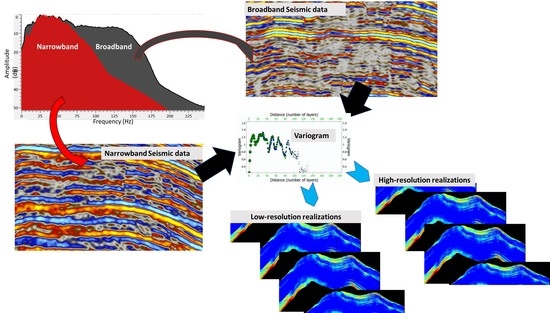
In an attempt to overcome this problem, geoscientists have adopted various approaches, one of which is the deconvolution of the seismic wavelet to obtain an acoustic impedance volume through a process known as seismic inversion. Of all the seismic inversion techniques, geostatistical inversion has proven excellent in resolving thin beds. Geostatistical inversion combines probability density functions (PDFs) and variogram models to simulate high frequencies in the output inversion product [6]. When a stochastic seismic inversion is successfully applied, it provides two important merits: an increase in resolution and an understanding of uncertainty by creating multiple equiprobable realizations of nonunique solutions [7]. Geostatistical inversion could aid in the delineation of thin-bedded reservoirs and provide more information about subsurface uncertainties. Reservoir properties and facies are important parameters to consider when characterizing reservoirs. Seismic inversion is now one of the most used techniques in reservoir modeling, characterization, and prediction. Stochastic inversion based on geostatistical theory can integrate various information and data and allow for the creation of high-resolution reservoir models [6]. Using the Bayesian procedure, multiple high-resolution realizations of elastic properties generate and classify facies probabilities to obtain the most detailed images of reservoir elements [8,9].

The authors of [9] investigated the difficulties and pitfalls of fault interpretation using seismic modeling and concluded that when high-resolution seismic data are available in addition to conventional seismic data, objective uncertainties decrease. Even though the resolution of seismic data has improved over the last few years, there are still significant limitations that impact interpretation. This constraint leads to imaging issues with complex subsurface geometries, as well as uncertainties in seismic qualities used for geologic modeling such as depth conversion [10,11]. As a result of this limitation caused by the limitedness of seismic bandwidth and the consequent tuning problem, seismic data have less of a restrictive effect on geostatistical inversion procedures, and the results increasingly resemble the results of kriging with well data [5]. However, these inversion methods involve a statistical relationship between the well and seismic elastic properties, which can affect the inversion outcome due to the difference in well and seismic frequencies. Moreover, most geostatistical approaches assume that the impedances from wells are statistically representative and that the spatial characteristics are correctly defined. For this presumption to hold, sufficient well control is required, which is usually not the case due to the paucity of wells at the hydrocarbon exploration stage. Vertical variograms are generally easy to derive from well logs, but there are rarely enough wells to accurately determine the lateral variogram. In several instances, statistical models rely on seismic impedance maps to infer the lateral parameters of geologic features [5].

Therefore, high-resolution seismic data are required to ensure an accurate prediction of the lateral continuity of facies [12] in their modeling of a geothermal reservoir, assuming that high-resolution volume shows considerable improvement over vintage images and leads to building an accurate complex 3D structural model. To enhance the seismic resolution, Ref. [13] proposed a spectral inversion algorithm that inverts the amplitude spectrum of the thin-bedded zero-phased seismic response to provide robust time-thickness estimates below tuning. The reflection coefficients are also estimated, which results in a sparse-reflectivity inversion. This was founded on the idea that any layer with a single reflection coefficient at the top and bottom can be represented as an impulse pair reflectivity series [14]. This reflection-coefficient pair can be divided into even and odd elements, with even components having equal magnitude and sign and odd components having equal magnitude but opposite sign. The weighted sums of the even and odd impulse pairs can be used to model multi-layers [15].

In this research, we applied the sparse-layer spectral inversion algorithm to enhance the resolution limit of Inas Field partial angle stacks seismic data. The enhanced seismic data were in turn used as input for geostatistical inversion to evaluate the Inas Field reservoir inter-well connectivity. The study was particularly focused on investigating a problem that led to the drilling of a dry hole in the Inas field. This problem is described in Section 1.1 below.

1.1. Field History and Problem Definition

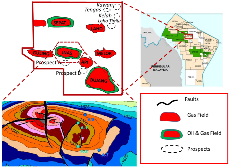
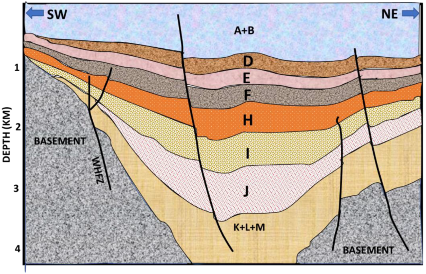
Inas Field, as shown in Figure 1, is in the offshore Malay Basin. It is an east–west trending asymmetrical compressional anticline with a gentle four-way dip closure against a major north–south trending normal fault. The Malay Basin is divided into chronostratigraphic units bounded by regional reflectors representing sequence boundaries or unconformities. These sequence stratigraphic units, which were subdivided into Groups A to M, have a strong relationship with the tectonic evolution of the Basin. The reservoir under consideration in this study is in the Group E sequences, deposited by progradational stacking of lacustrine channels and are bounded by erosional surfaces. A post-depositional compressional deformation led to the creation of anticlinal structures and faults that hosts hydrocarbon in the Inas Field. The predominant depositional environment for this zone is a lower coastal plain environment, and its lithologies are mainly channeled sandstone, claystone, and siltstone with coal seam intercalations.

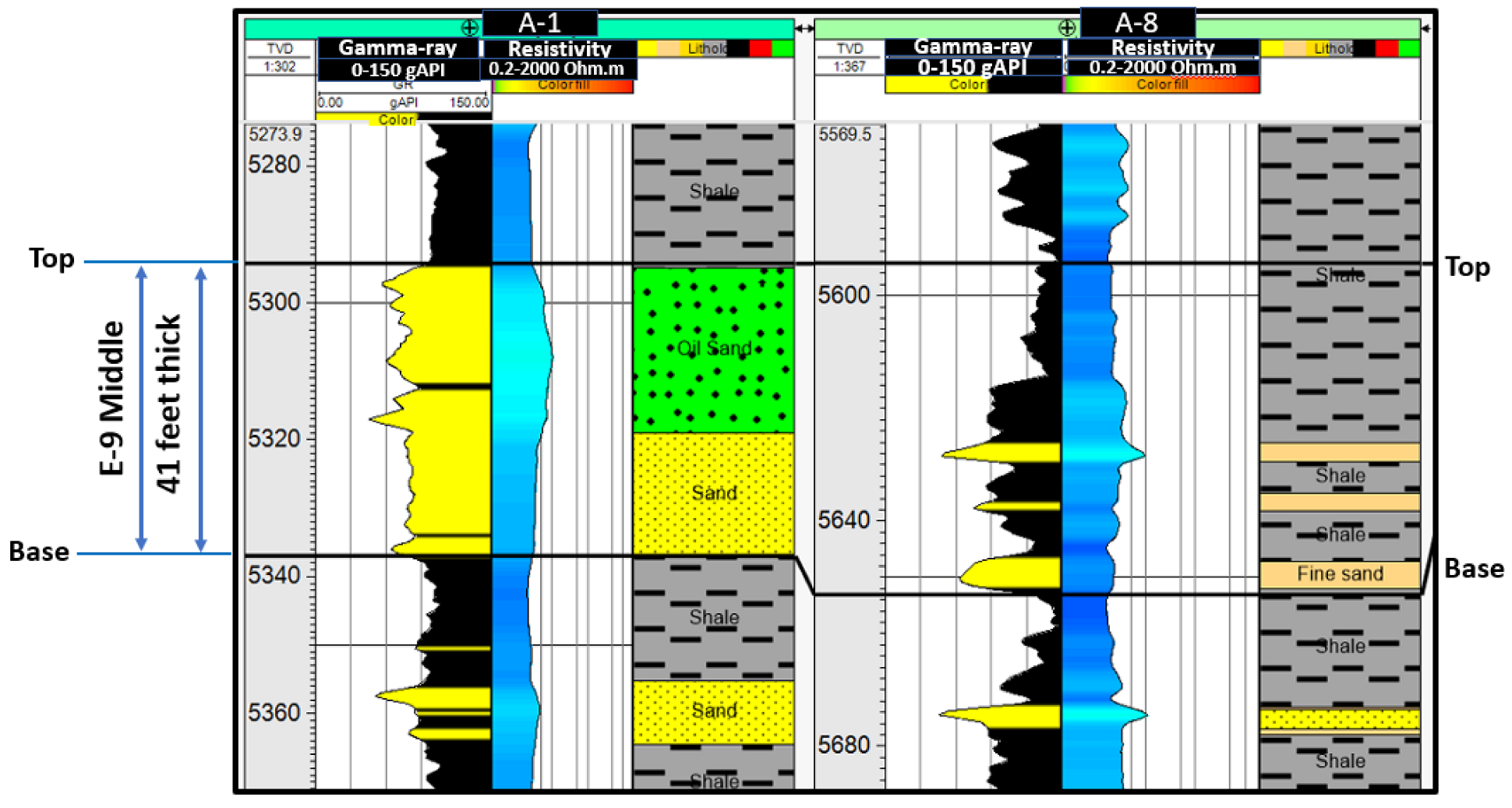
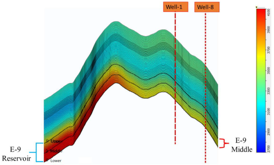
Inas Field is a gas field with minor oil rims at its eastern fault block, where a total of eight wells and a few sidetracks have been drilled to appraise the field. Some of these wells recorded successes, while some failed. One of the failed wells is the latest drilled well, A-8. This well was drilled to appraise the E-9 reservoir, which was oil-bearing in a nearby A-1 well Figure 1. The reservoir was divided into the upper, middle, and lower sublayers separated by thin shale beds. The net sand thickness in the E9-Middle is 41 feet Figure 2. Before the drilling of the A-8 well, spectral decomposition and geostatistical inversion studies were used to predict the probability of the presence of sand and hydrocarbon in the reservoir. After drilling, it was confirmed that the geostatistical inversion results gave an inaccurate prediction of the sand present in the E-9 layer. Unfortunately, the reservoir shaled out when spudded Figure 2. The inability of geostatistical inversion to predict the correct fluid content present was attributed to the thinly bedded pay sands coupled with the probable impacts of coal beds above it. From this observation, the geostatistical inversion study is known to be a useful technique for predicting reservoir distribution, but in this case, it was not able to determine the facies continuity of the reservoir. Therefore, the well was plugged and abandoned with a minor gas discovery at shallower reservoirs.

According to an internal report, the geology of Inas is complex and yet to be understood. There is therefore a need to meticulously study the field to understand more geologic details. Accurately interpreting seismic reflection data is one major factor for successful oil and gas exploration [16]. However, it is still difficult to tell the geologic stories recorded in seismic data volumes, especially when they are sub-seismic, as in Inas Field.

The assessment of lateral and vertical connectivity between reservoir sands is an arduous task, given the relatively low resolution of seismic data in most cases. Inas Field is even tougher owing to its extremely thin reservoir thickness. This thinness can be attributed to the coastal plain environment that is predominant in the field. Static reservoir connectivity analysis is virtually based on 3D facies or geo-body models defined by combining well data and inverted seismic impedances. The goal of this research paper is to answer some pertinent questions regarding the geostatistical prediction failure, investigating the impact of bandlimited seismic data on geostatistical inversion. For instance, if the A-1 well showed oil in an E-9-middle reservoir and a result from a geostatistical inversion study predicted the extension of that oil accumulation to the location of the A-8 well, why did the prediction fail? Could the prediction be more accurate if they had a seismic with a better resolution? Here, we improved the vertical resolution of the field’s seismic data by applying a sparse-layer spectral inversion to the seismic data. Both the bandlimited and the resultant broadband seismic data were used to perform a geostatistical inversion, and their results were compared.

1.2. Geologic Background of the Study Area

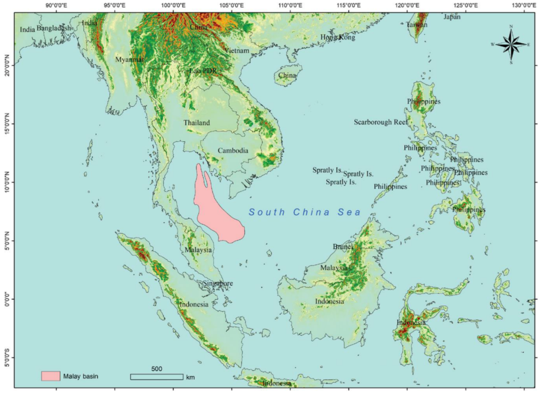
Inas Field is in the Northern Malay Basin, which is located in the southern part of the Gulf of Thailand, sandwiched between Vietnam to the northeast and Peninsular Malaysia to the southwest and bounded to the northwest by the Pattani Trough of Thailand and to the southeast by the West Natuna Basin of Indonesia, as shown in Figure 3. It has an aerial extent spanning about 80,000 square km with an average sediment thickness of about 14 km. The basin is elongated and trends NW–SE direction with a length and width of about 500 km and 250 km, respectively [17]. Different tectonic models have been proposed to explain the origin of the Malay basin, but the most widely used is the extrusion hypothesis proposed by [18], whereby the India–Asia collision has caused the reactivation of major strike-slip fault zones and the formation of extensional basins. The basin is believed to have formed during the Tertiary by crustal extension, and it is underlain by Pre-Tertiary basement rocks that were interpreted to be an offshore extension of the geology of eastern Peninsular Malaysia Basin [19].

The basin underwent inversion during the Middle to late Miocene, which led to the formation of compressional anticlines, reverse fault, inverted and uplifted half-graben, etc. The intensity of the inversion is greatest at the center of the basin and less intense at the basin flanks. In the axial region of the basin, large wrench-induced compressional anticlines were formed. These anticlines are mostly trending in the E–W direction, parallel to the basement normal faults bounding the syn-rift half grabens, which seem to control the location and geometry of the anticlines. The inversion anticline formed over the half-graben by a right-lateral shear that trended in the NW direction during the inversion phase of the basin [21]. The variation in thickness of the stratigraphic units across the anticlinal structure was used to determine the timing of the inversion anticline’s growth. The formation of the structures was contemporaneous with deposition, and the thickness of the syn-inversion stratigraphic units decreases towards the crest of the structure, as the depositional features are being deformed and eroded at the same time. The compression started around the time the top of Group H was being deposited, whereas the peak of deformation started during the deposition of Group E and continued till recent.

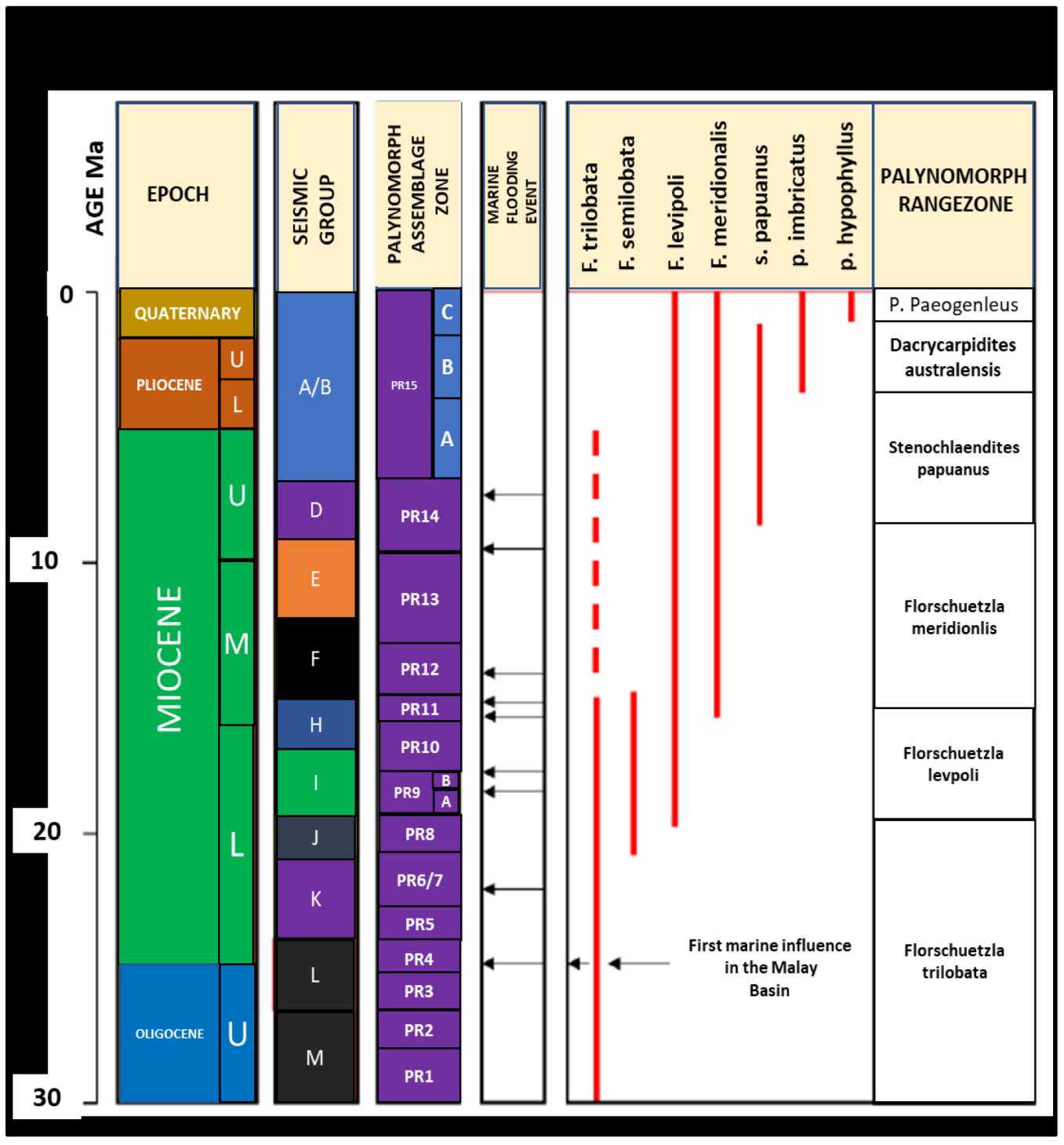
The Malay Basin is divided into chronostratigraphic units. These units were determined based on the seismic data, and each unit was designated as a Group, which is bounded by regional reflectors representing sequence boundaries or unconformities. The groups are named from A to M according to geologic age [22] (Figure 4).

The sequence stratigraphic units have a strong relationship with the tectonic evolution of the Basin. The evolution phases include (a) Syn-rift phase (Oligocene or Pre-Miocene), (b) tectonic/thermal phase (early to middle Miocene), (c) Subsidence phase (Late Miocene to Quaternary) [23]. The syn-rift phase represents the extensional phase of the basin development when sedimentation is controlled by faulting with the half grabens serving as main depocenters. This unit consists of successive sand and shale facies intercalations, which are mainly fluviolacustrine and alluvial deposits. Groups M to K fall within these units and have been interpreted to consist of the braided channel, fluvial, coastal plain, lacustrine delta, and lake deposits. The tectonic or thermal phase started after the Oligocene extensional faulting ceased about the time Groups L to D were deposited. The abundance of shale successive coal beds suggests that the shoreline at the time was close to the coast. There was a cyclic succession of marine, tidal estuarine, coastal, and fluvial deposits within this period. Groups E and D were deposited by the progradational stacking of lacustrine channels and bounded erosional surfaces (Figure 5). This phase was accompanied by compressional deformation.

The final phase was the phase of subsidence deposited around the late Miocene to Quaternary period. It was a period of no significant tectonic impact and gentle subsidence due to thermal cooling. This time, there was a full open marine transgression that led to the deposition of Groups A and B, which consisted of mainly shale and silt due to the low energy of the predominantly shallow marine environment.

The Northern Malay Basin’s petroleum system elements include a mature and effective source rock (coal and carbonaceous shale) of Groups H and I that provides the hydrocarbon charge to reservoirs in Groups E, D, and B [24]. The Northern Malay Basin’s hydrocarbon is primarily gas, trapped in the stratigraphically shallower units of Groups E, D, and B. This could be due to the regional overpressure seal in Group F below. These reservoir sequences are thought to have formed in continental, coastal, and shallow marine environments [20,24].

2. Materials and Methods

2.1. Data Presentation

2.1.1. Seismic Data

Post-stack time migrated full-stack seismic data, and the near-, mid-, and far-angle stacks with angle ranges of 5–15, 15–25, and 25–40 degrees were used in this study. The seismic data have a dominant frequency of 30 Hz at the reservoir interval and a bandwidth of 80 Hz. The sample interval is 2 ms with an approximate tuning thickness of 32 m at the reservoir interval. The horizon used as input in the inversion was interpreted using the full-stack data, whereas the geostatistical inversion was conducted with the angle stacks.

2.1.2. Well Data and Formation Tops

Eight wells were drilled in the field, but only four out of them penetrated the zone of interest. These wells are A-1, A-2, A-7, and A-8. All the required composite logs, such as compressional Sonic, Shear Sonic, Density, Gamma-ray, etc., were available and adequately covered the interval of interest. The Check shot data, the Vertical seismic processing data, and interval velocity data were provided and carefully integrated to perform a robust well-seismic tie. The formation tops of the reservoirs were provided, which was further quality checked to establish the inter-well correlations. These well tops were targeted during the well-seismic tie.

2.1.3. Core Data

Well A-8 and A-7 have core description data. These core data provided a detailed description of the lithofacies present in the reservoirs. These data were used to define the lithofacies log used in the facies classification analysis. It was later integrated with the plot of the compressional and shear velocities against the impedances to define the facies.

2.2. Geostatistical Inversion

Geostatistical inversion simulates high frequencies in the output inversion product utilizing probability density functions and variogram models. [7]. Since the geostatistical inversion method has been proven as a feasible and effective approach to solving the identification problems of super-thin reservoirs and reducing the risk of oilfield development and has a certain value for industrial application [25], we performed it again to re-evaluate whether other factors such as the bandlimitedness of the partial angle stack seismic data used as input in the previous inversion process impacted in the negative prediction outcome.

Geostatistical inversion entails combining seismic and geologic data from well-logs. Hence, an upscaling procedure is required to combine well-log data with seismic data. The prediction of the elastic properties of rocks at a lower frequency (Hz) (seismic or cross-well data) using a higher-frequency (kHz) elastic wave from logging data is known as upscaling [26]. The main parameter for well-log upscaling is the averaging window length (L), which is dependent on the wavelength and dominant frequency of the seismic data [27].

$$L\le \frac{\lambda dom}{N}=\frac{VSVmin}{N\ast fdom}$$

(1)

where: L = average window length, λdom = dominant wavelength of seismic data, VSVmin = minimum shear wave velocity (from well logs), N = factor from empirical research, and fdom = dominant frequency of the seismic wave.

Although achieving a high vertical resolution using the geostatistical inversion method does not depend directly on the seismic frequency, the averaging (upscaling) of the well-logs to the seismic frequencies directly depends on the seismic wave parameters, and this could affect how well the petro-elastic parameter from the wells and the seismic data are related. Therefore, using higher-resolution seismic data would invariably reveal better petro-elastic details than narrowband seismic data. Hence, the narrowband seismic data from Inas Field was broadened using a spectral inversion technique described below.

2.3. Application of Spectral Broadening Algorithm on Inas Seismic Data

The spectral inversion spectral broadening technique was proposed by [28]. The authors posited that the broadband spectrum of any reflectivity series within the analysis window (ranging from zero to the Nyquist frequency, the maximum frequency that can be observed in the data) can be clearly expressed as:

$$Sr\left(f\right)={{\displaystyle \sum }}_{n=0}^{k-1}\left(2r_e\left(n\right)·\cos \left(2\pi ·n·dt·f\right)+i2r_0\left(n\right)·\sin (2\pi ·n·dt·f\right)$$

(2)

where K is the number of impulse pairs, including all possible time thicknesses (+zero time thickness) in the analysis window of 2N + 1, while n·dt is half the time thickness of the impulse pair, with n varying from 0 to n, and dt is the sample rate. The coefficients (r_e) and (r₀) components can be calculated by applying the Basis Pursuit inversion algorithm postulated by [29].

The narrowband data spectrum, which is associated with a sum of reflector pairs, is the sum of frequency sinusoids multiplied by the wavelet spectrum. We must divide the wavelet to remove the wavelet overprint caused by the convolution of the reflectivity series with a limited band wavelet. As a result, to obtain reflectivity in the frequency domain, the seismic data spectrum (in the frequency domain) is divided by a known or estimated wavelet spectrum. The reflectivity spectrum of the bandlimited data is obtained by dividing it by the wavelet spectrum because the wavelet is known. Therefore, the spectrum is flattened, which equates to the wavelet spectral limit segment of the broadband reflectivity spectrum obtained by solving Equation (2). The layer reflectivity spectrum can then be extrapolated outside of the original seismic band by extending the spectra sinusoid. Equation (3) [14] connects the data spectral constraint (real and imaginary parts separately) and the sinusoidal elements of varying frequency periodicities now within the same spectral limit:

Sd = Φa + ε

(3)

where Sd is the deconvolved data spectrum, Φ is the kernel matrix of sinusoidal atoms, a is the reflection coefficients vector including r_e and r₀, and ε denotes the prediction error. Equation (3) is the frequency domain equivalence of the convolution model equation.

After the bandwidth is extended, we can calculate the resulting reflectivity series by inverting the reflectivity spectrum (in the frequency domain) to the time domain using Equation (4).

$$Sr\left(t\right)={{\displaystyle \sum }}_{n=0}^{k-1}\left(\left(r_e\left(n\right)+r_0\left(n\right)\right)b(t+n·dt\right)+\left(r_e\left(n\right)-r_0\left(n\right)\right)b\left(t-n·dt\right))$$

(4)

3. Results

3.1. Spectral Broadening Result

The procedure described above was applied to the entire volume, which resulted in an expanded bandwidth of 180 Hz. In Figure 6, the amplitude spectrum of the narrowband (original) data is overlaid on the amplitude spectrum of the calculated broadband data. It is observed that both low and high frequencies are added to the data. The spectral difference is about 100 Hz, and the spectrum of the broadband data is also flattened or whitened, thereby making thin reflectors resolvable [30,31].

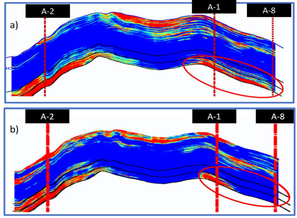
At the reservoir interval, the resolution limit (or tuning thickness) of the seismic data was initially calculated to be roughly 32 m, but the resolution limit became substantially reduced to 10 m in the broadband data without changing the real reflection signals. By reducing its tuning thickness to 10 m, it is now possible to correctly image the reservoir sands, which range from 10 m to 15 m. Figure 7a,b is the composite sections of both seismic volumes, sliced through the well intersections. It is seen in Figure 7a that the seismic loops are generally thick and do not capture tiny details. The composite section from the broadband (Figure 7b), however, shows a better vertical and lateral resolution.

3.2. Geostatistical Inversion Results

Following the broadening of the seismic bandwidth, two separate geostatistical inversions were performed with the resulting broadband and the original narrowband seismic data. For simplicity, these are referred to in this research as broadband and narrowband geostatistical inversions. The narrowband geostatistical inversion was carried out to understand what informed the decision of drilling the A-8 well, whereas the broadband inversion was to investigate if the earlier prediction failed because of poor resolution power of the original seismic data. Inas seismic vintage has very large coverage, but to reduce the run time and storage space of the inversion realizations, the area of interest for both the narrowband and the broadened seismic data were cropped out from the main seismic volume. Both seismic data have a sample rate of 2 ms, and the narrowband data have a bandwidth of 81 Hz, whereas the broadband (enhanced) seismic has a bandwidth of 180 Hz. The key inversion inputs included near, mid, and far seismic partial-angle-stack volumes with angle ranges of 5°–15°, 15°–25°, and 25°–40°, respectively. There were about eight wells drilled in Inas Field, but the interest area was penetrated by only four wells (A-1, A-2, A-7, and A-8). Additionally, they have the required P-wave velocity, S-wave velocity, and density logs. The seismic partial-angle stacks and well logs were quality checked properly and correlated through synthetic generation using statistical wavelets first and then wavelets from the well in preparation for the pre-stack stochastic inversion. All the synthetic seismic interval was tied to the seismic; however, more focus was placed on the reservoir of interest.

The geologic lithofacies were manually defined after proper biostratigraphic, chronostratigraphic, and lithostratigraphic correlations were conducted using the full-stack seismic, biostratigraphic, and lithologic logs data. The reservoir intervals and fluid types were determined from the well logs and validated by information from internal post-drilling reports. To further augment the results, we did a cross-plot of P-impedance and VP/VS ratio, which provided an optimum separation between the predefined lithofluid groups, and it matched very well with the manually interpreted lithofacies.

Figure 8 shows the geostatistical inversion workflow that was used in the study; however, before we proceeded with the inversion, we built an initial low-frequency guess model using the well data and interpreted the horizons of the target reservoirs. An initial guess model is a volume that defines a seismic parameter that has been interpreted, such as velocity, reflectivity, or impedance. It attempts to define the study area in more geological terms than just seismic reflectors and thus looks more like a stratigraphic model. This was used to constrain the inversion geocellular grids. 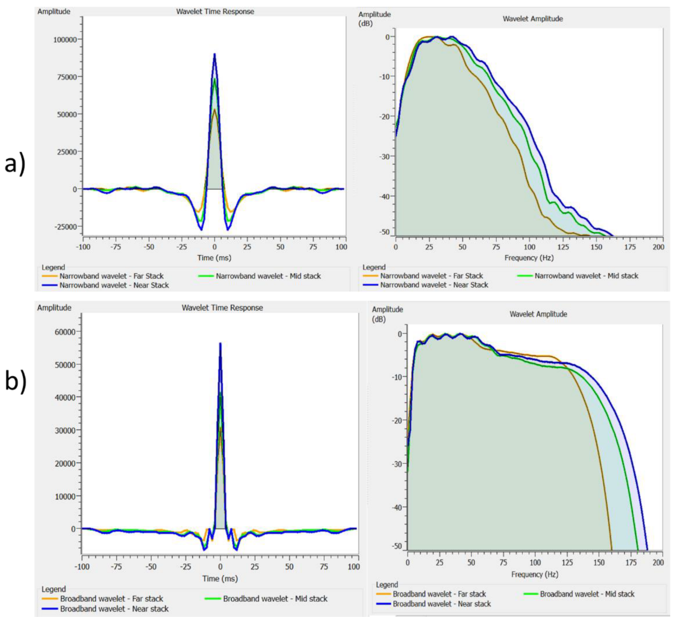Figure 9a shows the extracted wavelets from the narrowband partial stacks, while Figure 9b is from the broadband data. Notice that the amplitude spectrum of the narrowband wavelets is limited with the wavelet time response (lobe width) of 20 ms, whereas the amplitude spectrum of the broadband wavelets is expanded but has a short time response (lobe width) of only 10 ms. The short time width enables the resolution of finer reflectors. As expected, the wavelets’ amplitudes broadened from near to far angles. Due to differences in wavelet scaling between the initial guess model and geocellular grid models, we scaled the extracted wavelets used in geocellular grid modeling to match the initial guess model for each partial angle stack volume. This was achieved by scaling the wavelets with the initial guess model and the seismic data from which the wavelets were extracted. Each wavelet was scaled for each angle to create the geocellular model.

The geocellular grid Figure 10 was divided into 135 layers, each having a mean thickness of 1 ms. We combined 3 × 3 bins, and the bins were used only once for smoothing calculations by applying the mean operator. The macro layers were conformable and were constrained to a minimum thickness of 0.1 ms. The variogram analysis shown in Figure 11 was conducted using data from the partial angle stacks seismic and wells to estimate the vertical size and horizontal range. Stable model variograms were selected, and the vertical range of each macro-layer was defined using best-fit values. The horizontal and vertical variogram range values were set to 1500 and 6 m, respectively. The horizontal ranges were estimated from seismic data, whereas the vertical sizes were estimated from well data.

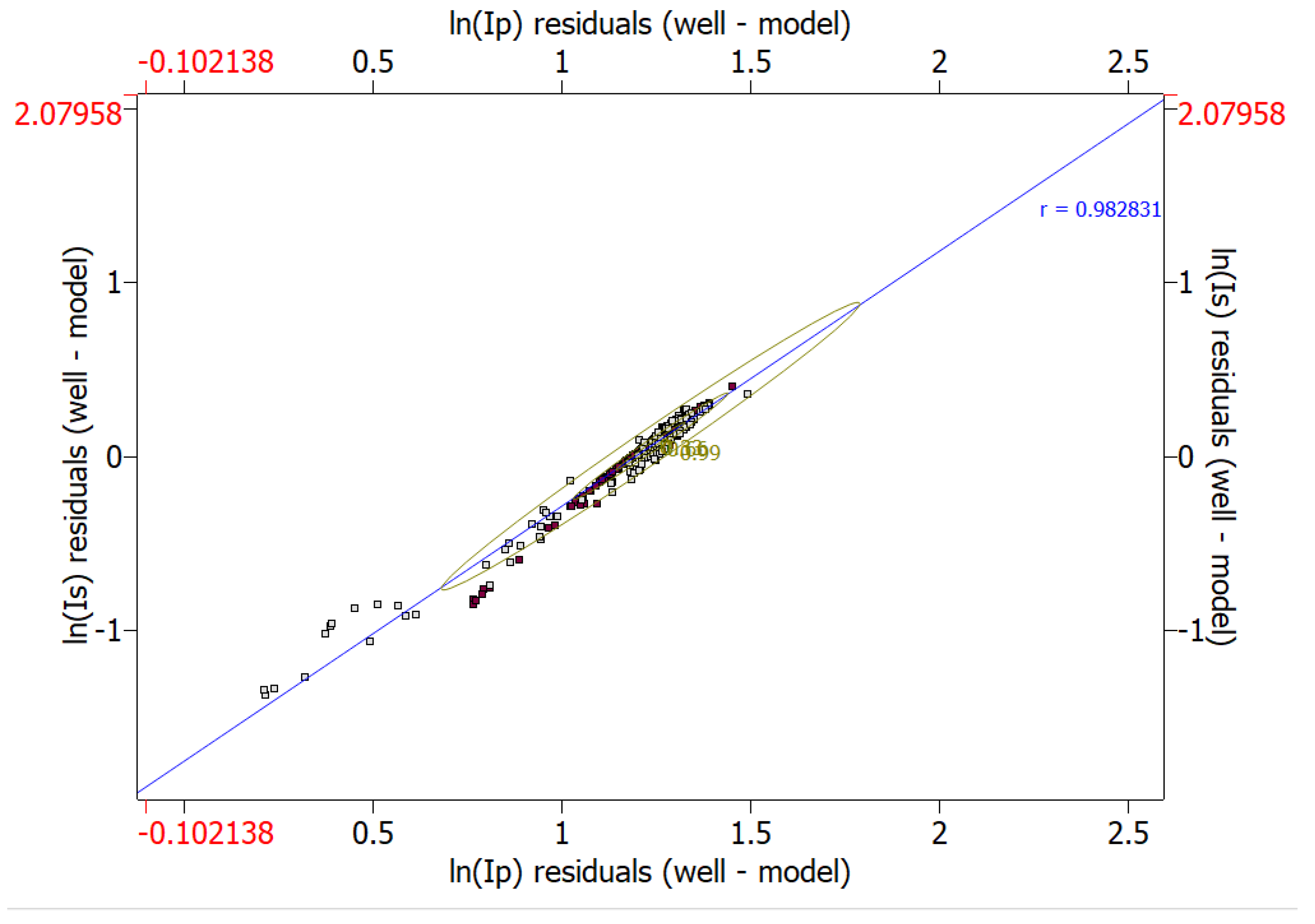
To quality check (QC) the variogram analysis, the natural logarithm of the shear and compressional impedance were cross-plotted, as shown in Figure 12, demonstrating the correlation of the plotted parameters. A higher correlation indicates a better result. The overall correlation coefficient of the impedance elastic parameters was 98 percent (r = 0.983). Twenty realizations of both P-impedance and S-impedance 3D volumes were generated using the narrowband and broadband seismic data.

3.3. Facies Classifications Methods

Using Bayesian methodology, the 20 realizations of the inverted elastic properties were further classified into facies and fluid probability volumes. The uncertainty in seismic inversion and rock physics should be reflected in the output probability cubes. To constrain the classification, we created probability density functions and used predefined lithofacies. To facilitate the creation of individual probability density functions for each distinguished lithofacies class, a P-impedance versus VP/VS ratio cross-plot was constructed using the posterior mean of high-frequency realizations. To demonstrate the high degree of conformance between the inverted and upscaled well-log attributes, the posterior mean was also superimposed by upscaled logs of the same properties.

Following the application of the facies classifications to all 20 high-frequency realizations using the Bayesian classification procedure, all facies’ realizations were ranked based on the net-to-gross ratio calculation, allowing the selection of three specific individual properties realizations representing P10, P50, and P90 possibilities [32]. The three property realizations were then used to generate the most likely facies cubes representing the P10, P50, and P90 quantiles. Because the individual facies cube generated from a single property realization represents one possible solution to the inverse problem, the inversion uncertainty can be captured by generating three facies’ cubes to represent the possible range of pay sand volumes [33].

The major advantage of a geostatistical inversion over other forms of inversion is an increase in resolution and an understanding of associated uncertainties through the creation of multiple equiprobable realizations of nonunique solutions. Since the geostatistical inversion is not solely controlled by the acoustic impedance features but also by other information, the number of possible solutions is reduced and nonuniqueness decreased [34].

The goal of various high-frequency realizations of inverted elastic properties is to measure subsurface uncertainty by expressing the non-uniqueness of the inversion process. With a predetermined uncertainty tolerance of 5%, each realization respected the petro-elastic constraints from the well, the seismic angle stacks, and the calculated geostatistical parameters. When overlaid by the well logs, the geostatistical inversion realizations of the impedance properties provided a good match to the unfiltered S-impedance and P-impedance logs, respectively, especially at the well locations. The thin-bedded reservoir facies were perfectly matched Figure 13.

4. Discussion

The major challenge with Inas Field is understanding its reservoirs’ connectivity and continuity. According to an internal report, the geology of the field is yet to be fully understood. This has posed a lot of challenges, and even more because of the limitedness of the data used in previous studies. This problem necessitated the adoption of the approaches used in this research. It is understood that Inas Field’s problem is unique, but the inversion technique is non-unique. Thus, we used the Bayesian approaches to resolve the seismic and petrophysical inversion problems [35], and the most probable realization was selected by ranking analysis and uncertainty quantification [24]. Figure 14a,b shows the P90 facies realizations for the broadband (Figure 14b) and the narrowband (Figure 14a) models. Generally, the result of the narrowband (Figure 14a) realization shows that the reservoirs are more continuous. This corroborates the results presented by [24], who integrated petro-elastic models, stochastic elastic inversion, and Bayesian probability classification to characterize the E-9 reservoirs. Their result agrees because they also used a narrowband seismic as input in their technique. Unfortunately, both outcomes (Figure 14a and [24]) do not represent the ground truth as confirmed from the well history. The broadband realization Figure 14b, on the other hand, shows that the sands are less continuous than indicated by the narrowband result. This is particularly evident in the E-9 middle sand. In the narrowband Figure 14a result, the facies extended from A-1 to A-8, whereas the broadband realization clearly shows that the reservoir tapered before A-8 (see red circles).

This facies continuity indicated by the narrowband inversion could have an impact due to the poor resolution of the input seismic data, resulting in an error in the prediction of the reservoir’s elastic properties [36], which affirms that poor seismic data quality affects the behavior of the seismic classification techniques, which may lead to unrealistic information of final facies prediction. However, when good-quality data are used for facies analysis, it provides an effective way to delineate the heterogeneity, continuity, and compartments within a reservoir [37].

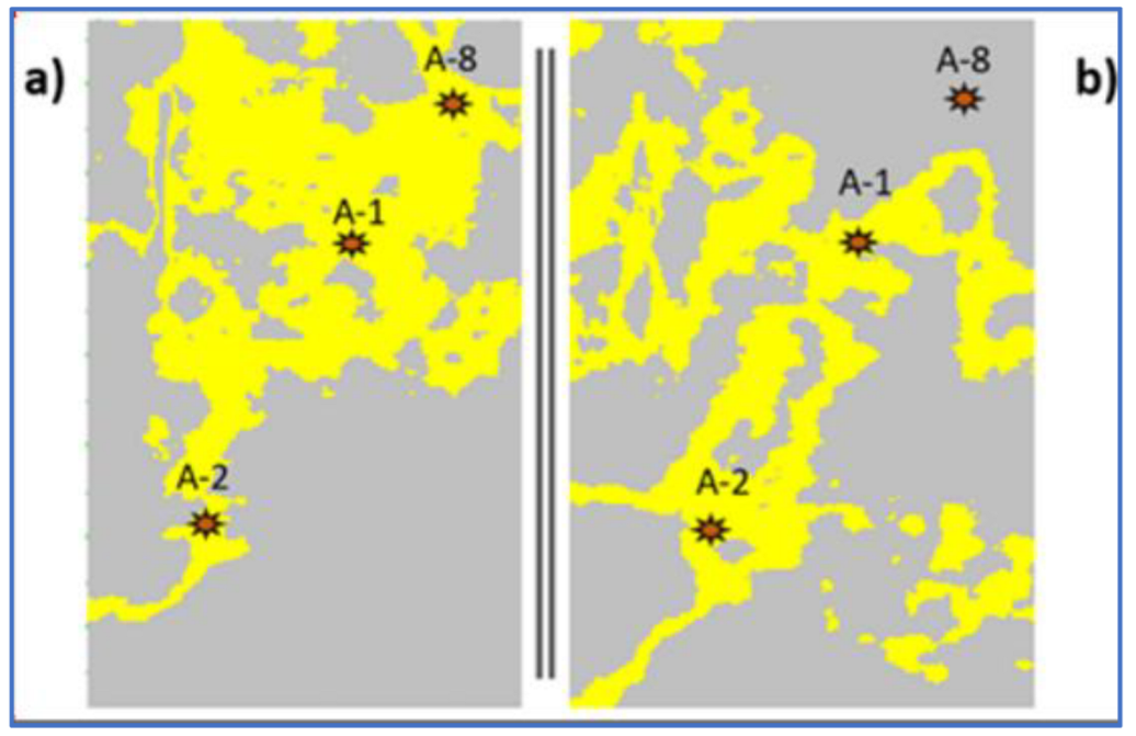
Figure 14 shows the sand facies distribution extracted within the reservoir zone at the cellular layer of 133. Figure 15a,b illustrates the extraction from the narrowband and the broadband inversions, respectively. It is observed from Figure 15a that the sand is well connected, continuous, and extends between A-1 and A-8 wells. Conversely, it looks disjointed in the sand distribution map of the broadband model (Figure 15b). This further confirms that the inter-well sand shaled out and did not extend to A8 in accordance with the well record. Some of such situations in which the reservoir geobodies appear ostensibly continuous are due to the inability of the seismic resolution to distinguish between tiny features [34]. This is often the result of a destructive interference problem, where the wavelet bandwidth overprints tiny geologic reflectors by combining them into one loop [38]. The inversion process attempts to remove this effect by dividing out the wavelet with a pre-estimated wavelet of similar bandwidth [14].

Since the seismic inversion process still depends on bandlimited wavelets [39] and the upscaling of well logs to the seismic scales also depends on the averaging window length [27], which is a function of the wavelength and dominant frequency of the input seismic data, the predictability of the lateral variations of seismic facies from well locations depends on the resolvability of the reservoir heterogenic properties. Optimum resolution is a prerequisite for extracting detailed, accurate geologic information from geostatistical inversion measurements, thus aiding not only in improved locations for hydrocarbon prospects (reservoir exploration) but also in the optimum distribution of well locations within a potential field (reservoir analysis) prior to development drilling [40].

By applying sparse-layer spectral inversion to the input partial angle stacks, we recovered the original earth reflectivity spectrum of the data. This was based on the principle that all transient signals have an unending frequency response that can be predicted to some extent if enough of the spectrum is sampled [14,16]. This process shortened the seismic wavelength and increased its dominant frequency across the entire volume. Using this new approach has demonstrated a better reservoir characterization compared to the use of the traditional narrowband seismic data. By examining the results, we conclude that the broadband geostatistical inversion, which produced a suite of equiprobable realizations, allowed a more accurate interpretation of the sand bodies that constitute the reservoir, as well as their individualization and continuity.

5. Conclusions

The broadband geostatistical inversion efficiently improved the reservoir characterization process by not only producing an accurate estimation of the lateral extent of the reservoir heterogeneities but also generating outcomes that help us understand why other geostatistical inversion analyses of the target reservoir were misleading. Based on this outcome, we conclude that:

• The tuning effects of bandlimited data can affect the result of a geostatistical inversion and result in wrong facies prediction;
• Using broadband partial angle stacks as an input in the geostatistical inversion process gave an accurate facies prediction and indicated the actual extent of the predicted reservoir facies;
• The recommendation to drill the A-8 well was based on misleading results due to the narrowband seismic data used in the inversion process;
• Generally, the result from the enhanced seismic data shows that Inas Field reservoirs are extremely discontinuous, which is typical of a coastal plain setting, being the dominant paleoenvironment of the reservoir zone.

Finally, it is important to state that the proposed method in this research is site-specific and has not been satisfactorily tested in all sites; however, it can be adopted in similar fields and situations but not the model itself.

6. Further Application

6.1. Exploration of Deep Reservoirs

Seismic resolution decreases with depth because of the earth filtering effect and several other factors [5]. The result of this is that seismic data often have a poorer resolution in deeper sections, resulting in the under-exploration of deep reservoirs [41], while using seismic attributes for fracture and porosity detection. We also noted that a decrease in density and slowdown in acoustic propagation velocity yields a relative drop in P-wave impedance, thereby reducing our understanding of inter- and intra-reservoir properties, especially at deep reservoirs, [42]. The application of sparse-layer spectral inversion and the use of the resulting broadband seismic for geostatistical inversion, as discussed in this research, can help in the delineation of such hidden subtle reservoir features.

6.2. Prediction of Unconventional Reservoirs for CO₂ Storage

This method, in addition to predicting conventional reservoirs, can be used to investigate CO₂ storage potential in an unconventional reservoir. The authors of [43] used diverse methods to assess CO₂ storage potential and injectivity in the Bakken Formation and deduced that adsorption outpaces molecular diffusion in determining the CO₂ injection rate in an unconventional reservoir. This finding implies that shale reservoirs are suitable for potential CO₂ storage. In addition, [44] developed a 1.9 m 0.2 m 0.2 m numerical model to simulate CO₂/N₂ flue gas injection in shale reservoirs with different pore size distributions of shale. Their findings revealed that the amount of CO₂ storage and enhanced oil recovery is dependent on the pore size distribution, which is indirectly dependent on the reservoir rock facies. Using broadband seismic data and the geostatistical inversion technique, it is possible to accurately predict the continuity of a shale reservoir, which has an advantage for CO₂ storage over conventional reservoirs [45]. This technique can be combined with the hydrocarbon prediction approaches proposed by [46,47]. An optimization of the shale and pore fluid separation using attenuation attributes proposed by [48], could help in lithofacies identification [49] and the prediction of CO₂ reservoir sealability.

References

1. Romero-Ruiz, A.; Linde, N.; Keller, T.; Or, D. A review of geophysical methods for soil structure characterization. Rev. Geophys. 2018, 56, 672–697. [Google Scholar] [CrossRef] [Green Version]
2. Lesmes, D.; Friedman, S. Relationships between the electrical and hydrogeological properties of the rocks and soils. In Hydrogeophysics; Rubin, Y., Hubbard, S.S., Eds.; Springer: Dordrecht, The Netherlands, 2005; pp. 87–128. [Google Scholar]
3. Mavko, G.; Mukerji, T.; Dvorkin, J. The Rock Physics Handbook: Tools for Seismic Analysis of Porous Media; Cambridge University Press: Cambridge, UK, 2009. [Google Scholar]
4. Rubino, J.G.; Velis, D.R. Thin-bed prestack spectral inversion. Geophysics 2009, 74, R49–R57. [Google Scholar] [CrossRef]
5. Simm, R.; Bacon, M. Seismic Amplitude, an Interpreter’s Handbook; Cambridge University Press: Cambridge, UK, 2014; pp. 32–36. [Google Scholar]
6. Liu, X.; Li, J.; Chen, X.; Li, C.; Guo, K.; Zhou, L. A stochastic inversion method integrating multi-point geostatistics and sequential Gaussian simulation. Chin. J. Geophys. 2018, 61, 2998–3007. [Google Scholar] [CrossRef]
7. Pendrel, J. Seismic inversion—The best tool for reservoir characterization. CSEG Rec. 2001, 26, 18–24. [Google Scholar]
8. Grana, D.; Fjeldstad, T.; Omre, H. Bayesian gaussian mixture linear inversion for geophysical inverse problems. Math. Geosci. 2017, 49, 493–515. [Google Scholar] [CrossRef]
9. Faleide, T.S.; Braathen, A.; Lecomte, I.; MulrooneyIvar, M.J.; Midtkandal, I.; Bugge, A.J.; Planke, S. Impacts of seismic resolution on fault interpretation: Insights from seismic modelling. Tectoonophysics 2021, 816, 229008. [Google Scholar] [CrossRef]
10. Bond, C.E. Uncertainty in structural interpretation: Lessons to be learnt. J. Struct. Geol. 2015, 74, 185–200. [Google Scholar] [CrossRef] [Green Version]
11. Schaaf, A.; Bond, C.E. Quantification of uncertainty in 3-D seismic interpretation: Implications for deterministic and stochastic geomodeling and machine learning. Solid Earth 2019, 10, 1049–1061. [Google Scholar] [CrossRef] [Green Version]
12. Salaun, N.; Toubiana, H.; Mitschler, J.; Gigou, G.; Carriere, X.; Maurer, V.; Richard, A. High-resolution 3D seismic imaging and refined velocity model building improve the image of a deep geothermal reservoir in the Upper Rhine Graben. Lead. Edge 2020, 39, 857–863. [Google Scholar] [CrossRef]
13. Puryear, C.; Castagna, J.P. Layer-thickness determination and stratigraphic interpretation using spectral inversion: Theory and application. Geophysics 2008, 73, R37–R48. [Google Scholar] [CrossRef]
14. Liang, C.; Castagna, J.P.; Zavala, R.T. Tutorial: Spectral bandwidth extension—Invention versus harmonic extrapolation. Geophysics 2017, 82, W1–W16. [Google Scholar] [CrossRef]
15. Marfurt, K.J.; Kirlin, R.L. Narrow-band spectral analysis and thin-bed tuning. Geophysics 2001, 66, 1274–1283. [Google Scholar] [CrossRef] [Green Version]
16. Chopra, S.; Castagna, J.; Portniaguine, O. Seismic Resolution and Thin-Bed Reflectivity Inversion; Fusion Petroleum Technologies, Inc.: The Woodlands, TX, USA; University of Houston: Houston, TX, USA, 2006; pp. 19–23. [Google Scholar]
17. Arshad, A.R.M.; Mhd, D.; Tjia, H.D. 1995, A deep seismic section across the Malay Basin: Processin of data and tectonic interpretation. In Geological Society of Malaysia Petroleum Conference; Warta Geologi: Kuala Lumpur, Malaysia, 1995; p. 412. [Google Scholar]
18. Tapponnier, P.; Peltzer, G.; Le Dain, A.Y.; Armijo, R.; Cobbold, P. Propagating extrusion tectonics in Asia: New insights from simple experiments with pasticine. Geology 1982, 10, 611–616. [Google Scholar] [CrossRef]
19. Mansor, Y.M.; Rahman, A.H.; Menier, D.; Pubellier, M. Structural evolution of Malay Basin, its link to Sunda Block tectonics. Mar. Pet. Geol. 2014, 58, 736–748. [Google Scholar] [CrossRef]
20. Babikir, I.A.; Salim, A.M.; Ghosh, D.P. Lithogeomorphological facies analysis of Upper Miocene coal-prone fluviodeltaic reservoirs, Northern Malay Basin. Interpretation 2019, 7, T565–T579. [Google Scholar] [CrossRef]
21. Tjia, H.D. Inversion tectonics in the Malay Basin: Evidence and time of events. Bull. Geol. Soc. Malays. 1994, 36, 119–126. [Google Scholar]
22. Madon, M.B.H. Depositional setting and origin of berthierine oolitic ironstones in the lower Miocene Terengganu shale, Tenggol Arch, offshore peninsular Malaysia. J. Sediment. Petrol. 1992, 65, 899–916. [Google Scholar]
23. Madon, M.; Abolins, P.; Hassan, R.A.; Yakzan, A.M.; Yang, J.S.; Zainal, S.B. Petroleum systems of the Northern Malay Basin. Pet. Geol. Conf. Exhib. Bull. 2004, 49, 125–134. [Google Scholar] [CrossRef] [Green Version]
24. Babasafari, A.B.; Ghosh, D.P.; Salim, A.M.A.; Kordi, M. Integrating petroelastic modeling, stochastic seismic inversion, and Bayesian probability classification to reduce uncertainty of hydrocarbon prediction: Example from Malay Basin. Interpretation 2020, 8, SM65–SM82. [Google Scholar] [CrossRef]
25. Shen, H.; Liang, X.M.; Qin, D.H. Application of Geostatistical Inversion for Super Thin Reservoir Prediction. In Proceedings of the 77th EAGE Conference and Exhibition, Madrid, Spain, 1–4 June 2015; European Association of Geoscientists & Engineers: Houten, The Netherlands, 2015; pp. 1–5. [Google Scholar] [CrossRef]
26. Bayuk, I.O.; Ammerman, M.; Chesnokov, E.M. Upscaling of elastic properties of anisotropic sedimentary rocks. Geophys. J. Int. 2008, 172, 842–860. [Google Scholar] [CrossRef] [Green Version]
27. Kozubal, A.; Wawrzyniak-Guz, K. Upscaling of Well-log Data to Seismic Scale–Comparison of Backus Theory and Running Average Method Results. In Proceedings of the 77th EAGE Conference and Exhibition, Madrid, Spain, 1–4 June 2015; European Association of Geoscientists & Engineers: Houten, The Netherlands, 2015; Volume 2015, pp. 1–3. [Google Scholar] [CrossRef]
28. Zhang, R.; Castagna, J.P. Seismic sparse-layer reflectivity inversion using basis pursuit decomposition. Geophysics 2011, 76, R147–R158. [Google Scholar] [CrossRef] [Green Version]
29. Fraser, G.B.; Neep, J. Increasing seismic resolution using spectral blueing and colored inversion: Cannonball field, Trinidad. In SEG Technical Program Expanded Abstracts 2004; Society of Exploration Geophysicists: Tulsa, OK, USA; pp. 1794–1797.
30. Zabihi Naeini, E.; Sams, M.S. Accuracy of wavelets, seismic inversion, and thin-bed resolution. Interpretation 2017, 5, T52–T530. [Google Scholar] [CrossRef] [Green Version]
31. Moyen, R.; Doyen, P.M. Reservoir connectivity uncertainty from stochastic seismic inversion. In SEG Technical Program Expanded Abstracts 2009; Society of Exploration Geophysicists: Tulsa, OK, USA; pp. 2378–2382.
32. El-Behiry, M.G.; Dahroug, S.M.; Elattar, M. Application of geostatistical seismic inversion in reservoir characterization of Sapphire gas field, offshore Nile Delta, Egypt. Lead. Edge 2019, 38, 474–479. [Google Scholar] [CrossRef]
33. Sancevero, S.S.; Remacre, A.Z.; Mundim, E.C.; de Souza Portugal, R. Application of Stochastic Inversion to Reservoir Characterization Process. Earth Sci. Front. 2008, 15, 187–195. [Google Scholar] [CrossRef]
34. Figueiredo, L.P.; Grana, D.; Bordignon, F.L.; Santos, M.; Roisenberg, M.; Rodrigues, B.B. Joint Bayesian inversion based on rock-physics prior modeling for the estimation of spatially correlated reservoir properties. Geophysics 2018, 83, M49–M61. [Google Scholar] [CrossRef]
35. Coléou, T.; Poupon, M.; Azbel, K. Unsupervised seismic facies classification: A review and comparison of techniques and implementation. Lead. Edge 2003, 22, 942–953. [Google Scholar] [CrossRef]
36. Song, C.; Liu, Z.; Wang, Y.; Li, X.; Hu, G. Multi-waveform classification for seismic facies analysis. Comput. Geosci. 2017, 101, 1–9. [Google Scholar] [CrossRef]
37. Sheriff, R.E. Encyclopedic Dictionary of Applied Geophysics, 4th ed.; Society of Exploration Geophysicists: Tulsa, OK, USA, 2002. [Google Scholar]
38. Maurya, S.P.; Singh, N.P.; Singh, K.H. Seismic Inversion Methods: A Practical Approach; Springer: New York, NY, USA, 2020; pp. 1–18. [Google Scholar]
39. Berkhout, A.J. Seismic resolution: A key to detailed geologic information. World Oil 1985, 201. [Google Scholar]
40. Somasundaram, S.; Mund, B.; Sharda, R. Seismic attribute analysis for fracture detection and porosity prediction: A case study from tight volcanic reservoirs, Barmer Basin, India. Lead. Edge 2017, 36, 874–960. [Google Scholar] [CrossRef]
41. Jia, B.; Chen, Z.; Xian, C. Investigations of CO2 storage capacity and flow behavior in shale formation. J. Pet. Sci. Eng. 2022, 208, 109695. [Google Scholar] [CrossRef]
42. Nizarul, O.; Hermana, M.; Bashir, Y.; Ghosh, D.P. Improving thin bed identification in Sarawak Basin field using short time Fourier transform half Cepstrum (STFTHC) method. IOP Conf. Ser. Earth Environ. Sci. 2016, 30, 012003. [Google Scholar] [CrossRef] [Green Version]
43. Pu, H.; Wang, Y.; Li, Y. How CO2-storage mechanisms are different in organic shale: Characterization and simulation studies. Spe. J. 2018, 23, 661–671. [Google Scholar] [CrossRef]
44. Ansari, H.; Trusler, M.; Maitland, G.; Piane, C.D.; Pini, R. The gas-in-place and CO2 storage capacity of shale reservoirs at subsurface conditions. In Proceedings of the 15th Greenhouse Gas Control Technologies Conference, Online, 15–18 March 2021. [Google Scholar]
45. Leslie, W.C.; Kadir, M.K.A.; Ghani, M.A.; Kader, M.S.; Zakaria, A.A.; Abdullah, C.S.H.; Daud, R. Malay and Penyu Basins Regional Study; Unpublished Report; Petronas Carigali: Kuala Lumpur, Malaysia, 1994; pp. 1992–1994. [Google Scholar]
46. Hermana, M.; Ghosh, D.P.; Sum, C.W. Discriminating lithology and pore fill in hydrocarbon prediction from seismic elastic inversion using absorption attributes. Lead. Edge 2017, 36, 902–909. [Google Scholar] [CrossRef]
47. Sambo, C.H.; Hermana, M.; Babasari, A.; Janjuhah, H.T.; Ghosh, D.P. Application of Artificial Intelligence Methods for Predicting Water Saturation from New Seismic Attributes. In Offshore Technology Conference Asia; OnePetro: Richardson, TX, USA, 2018. [Google Scholar]
48. Hermana, M.; Ghosh, D.P.; Sum, C.W. Optimizing the lithology and pore fluid separation using attenuation attributes. In Offshore Technology Conference Asia; OnePetro: Richardson, TX, USA, 2016. [Google Scholar]
49. Ngui, J.Q.; Hermana, M.; Ghosh, D.; Wan Yusof, W.I. Integrated study of lithofacies identification—a case study in X field, Sabah, Malaysia. Geosciences 2018, 8, 75. [Google Scholar] [CrossRef] [Green Version]
Figure 1. Base map of the study field, Peninsular Malaysia. A-1 and A-8 are the wells in the field. A-8 was drilled to appraise the extent of the reservoir encountered by A-1. The black lines indicate faults.
Jmse 10 00727 g001
Figure 2. A-1 and A-8 wells showing the E-9 middle reservoir (highlighted). The reservoir thickness is 41 feet.
Jmse 10 00727 g002
Figure 3. The location map of the Malay Basin (left), which is located offshore the peninsular Malaysia in the South China Sea [20].
Jmse 10 00727 g003
Figure 4. Schematic Geologic cross-section, showing the sequence stratigraphic Groups and geologic structures of Malay Basin (Redrawn after [23]).
Jmse 10 00727 g004
Figure 5. Stratigraphic scheme of the Malay Basin. The seismic groups correlated to the main palynomorphs assemblage zones (PR). The marine flooding events are also indicated (modified after [23]).
Jmse 10 00727 g005
Figure 6. Inas Field Seismic data spectrum showing the narrowband (green) and broadband (blue) spectra at time 1000–1500 ms.
Jmse 10 00727 g006
Figure 7. (a) Composite section of the narrowband (8–80 Hz) seismic volume through the A-1, A-2, and A-8 wells showing the E-9 reservoirs. (b) Composite section of the broadband (2.5–180 Hz-enhanced) seismic volume through the A-1, A-2, and A-8 Wells showing the E-9 reservoirs (black horizons).
Jmse 10 00727 g007
Figure 8. The geostatistical inversion workflow that was used in the study.
Jmse 10 00727 g008
Figure 9. (a) Narrowband seismic wavelets used for geocellular modeling. (b) Broadband seismic wavelets used for geocellular modeling.
Jmse 10 00727 g009
Figure 10. Geocellular grid model showing impedance distributions, well intersections, and reservoir of interest.
Jmse 10 00727 g010
Figure 11. Variogram analysis plot: the blue circles are the experimental variogram from P-impedance, whereas the green balls are experimental variogram from shear impedance.
Jmse 10 00727 g011
Figure 12. Correlation coefficient plot of the natural logarithm of p-impedance versus s-impedance.
Jmse 10 00727 g012
Figure 13. High-frequency P-90 geostatistical inversion realization showing a good match with the overlaid P-impedance well log. The impedance contrasts of the inversion are strongly correlated to the well log signature.
Jmse 10 00727 g013
Figure 14. P-90 Facies volumes applied on the high-frequency geostatistical inversion realizations: (a) narrowband (original) seismic data used as input and (b) broadband (enhanced) seismic data as input. The encircled (red) portions show facies change towards A-8 in (a), while (b) shows continuous facies.
Jmse 10 00727 g014
Figure 15. Sand and shale distribution maps of the middle of E9 at the geocellular layer of 133. (a) Sand/shale distribution from the narrowband geostatistical inversion. (b) Sand/shale distribution from the broadband geostatistical inversion.
Jmse 10 00727 g015
Publisher’s Note: MDPI stays neutral with regard to jurisdictional claims in published maps and institutional affiliations.