
Numerical Investigation of Breaking Focused Waves and Forces on Coastal Deck Structure with Girders


Civil Engineering Department, Indian Institute of Technology Bombay, Powai 400076, India
*
Author to whom correspondence should be addressed.
J. Mar. Sci. Eng. 2022, 10(6), 768; https://0-doi-org.brum.beds.ac.uk/10.3390/jmse10060768
Submission received: 18 March 2022
/
Revised: 13 May 2022
/
Accepted: 18 May 2022
/
Published: 1 June 2022
(This article belongs to the Special Issue Performance of Transportation Systems Subjected to Extreme Hydrodynamic Events)
Abstract
:In the present study, breaking focused wave groups were simulated using open-source Computational Fluid Dynamics model REEF3D in order to investigate the breaking wave impact on scaled (1:10) two-dimensional coastal deck structure with girder. The effect of environmental parameters, such as bottom slope and wave steepness on the breaking and geometric properties of high-crested spilling breakers, was investigated. The effect of the wave breaking location on the impact forces acting on the deck structure located at different airgap positions was studied for three wave impact scenarios: (i) when the wave breaking starts, (ii) when a slightly overturning crest is formed, and (iii) when the wave breaks and a fully overturning crest is formed just before hitting the preceding trough. The peak horizontal impact force was found to be higher when the wave breaks ahead of the structure and the overturning wave crest hits the deck positioned above the still water level. Additionally, the peak vertical impact force attains the peak when the deck is placed at the still water level for different stages of breaking. The peak horizontal impact force shows a parabolic trend, whereas the peak vertical impact forces show a decreasing linear trend with an increase in airgap. Finally, force coefficients are derived for calculating the peak impact force on deck with girders subjected to high-crested spilling breakers.
1. Introduction
Breaking waves can cause an enormous impact on coastal structures due to the sudden impingement of water mass against the structure and due to complex free surface transformations during the breaking process. An insight into the velocity and impact pressure variation can help us to obtain a deep understanding of the wave breaking process. Coastal structures are subjected to damages arising from sudden slamming caused by breaking waves. Wave breaking effects on vertical structures such as seawalls and breakwater were widely investigated [1,2]. The Indian Ocean Tsunami (2004) caused severe damage to the seawall, wharf deck, jetties and bridges. The wave impact on bridge decks was widely studied after hurricane Katrina which alone damaged 44 bridges along the Gulf Coast region [3,4].
Similarly, various hurricanes [Wilma and Rita (2005), Ike (2008), Irma (2017), and Michael (2018)] and tsunamis [Great East Japan Tsunami (2011), and Palu Tsunami (2018)] caused tremendous damage to the bridge decks, which demands detailed research in this area [5]. The storm surges were associated with a sudden rise in water level increasing the water depth over which extreme waves propagate and hit the decks, causing an impact. Large-crested waves on top of the surge impact the bridge decks during storm surges. The wave impact on submerged, partially submerged and completely elevated bridge decks were investigated both experimentally and numerically in the past [6,7,8,9,10]. The wave breaks on the structure when the deck is above the water level compared to submerged decks. The impact on the submerged deck showed a smooth force–time history and exhibited large fluctuations for decks located above the still water level [11]. An arbitrary Lagrangian–Eulerian (ALE) numerical method with a multi-phase compressible formulation is used for the development of three-dimensional hydrodynamic models by [12], which is validated for fluid structure interaction involving two-phase flow. Solitary [13], regular Stokes and focused waves were widely used experimentally and numerically to study the impact on coastal structures. Extreme waves with high crests were found to be better represented by focused waves [14] and used to investigate the impact on coastal decks [15]. These large-crested waves break due to shoaling as they approach the shore and may break due to the action of wind. The breaking of such waves creates spilling breakers during storm scenarios. Thus, it is crucial to understand the breaking wave impact on the coastal decks, as the large-crested waves undergoing spilling breakers are common.
The breaking wave geometry and kinematics were studied using solitary [16], regular [8] and irregular waves [17] over beach slopes for different wave steepness. These studies consider spilling and plunging breakers and their impact on vertical cylinders. The environmental parameters such as water depth, beach slope and wave steepness effects were investigated both experimentally and numerically. The limiting steepness for Stokes waves in deep water goes up to 0.443 as per Stokes theory. Ref [18] observed the limiting steepness up to 0.41 for spilling breakers generated in a convergent channel. The local wave geometry was also found to be a better alternative to define breaking, which includes the wave crest front steepness, wave crest rear steepness, and vertical and horizontal asymmetry. These parameters defining the local geometry were first introduced by [19]. According to their study, breaking crest front steepness was reported to vary between 0.32 and 0.78, whereas the vertical and horizontal asymmetry factors are 2.0 and 0.9, respectively. Ref [20] also observed the breaking wave profiles and found the crest front steepness between 0.25 and 0.55, whereas the vertical and horizontal asymmetry parameters are 2.14 and 0.77, respectively. Additionally, the averaged value of crest front steepness was reported to be 0.38 for spillers and 0.61 for plungers. The wave steepness and the local wave parameters were in different ranges for Stokes, solitary and irregular wave breaking. For Stokes second-order waves in deep water, the crest front and rear steepness were 0.40, whereas the vertical and horizontal asymmetry parameters were 1.0 and 0.61, respectively. Experimental investigations of breaking wave impact on vertical cylinders [21,22,23] suggest that the impact force due to breaking wave depends on the breaking wave geometry and wave kinematics. Additionally, the position of the structure with respect to the breaking location induces higher impulsive impact pressure. Similarly, understanding of the wave kinematics during the impact on deck with girders can help in understanding the impact pressure and forces acting on the structure, which require detailed investigation.
Numerical modelling of the breaking wave can be carried out by adopting suitable sea bed slopes or by using the focused wave concept [24,25]. The focused wave generated using nonlinear wave–wave interaction was used for generating larger wave heights by constructive interference. These large waves generated using wave focusing were used for breaking wave generation [26,27,28]. A detailed review of breaking studies using the focused wave concept was described in [29]. Ref [30] performed experiments on wave groups and observed that the breaking of wave groups depends on the local wave geometry. A detailed investigation was further carried out [31] to study the wave characteristics of wave groups and local breaking waves. The time and length scale of active breaking, the energy dissipation and the strength of breaking were numerically investigated. The numerical studies were carried out mainly using the Reynolds Averaged Navier–Stokes equations with suitable free surface capture methods. Breaking wave impact due to focused wave generated using the JONSWAP spectrum as input was investigated by [32] using openFOAM. Ref [33] computed breaking wave impact pressures on a tripod structure subjected to breaking focused waves under three impact conditions using the commercial software ANSYS CFX. The same concept of the focused wave was used to generate wave breaking in intermediate water to study the breaking wave kinematics on monopile structures [32,34] and flat bridge deck structures of rectangular cross section [35,36].
An open source CFD model, REEF3D has been successfully used by many researchers to simulate breaking waves and investigate the impact on structures [37,38]. Ref [11] used this model to study the solitary wave impact (including slamming and quasi-static force) on a coastal bridge deck with girder. The numerical model was further used for studying the non-breaking and breaking focused wave impact on an offshore deck [39]. However, studies of breaking wave impact on complex coastal decks with girders are not available. Hence, it is important to investigate the breaking wave kinematics during the non-linear interaction of a breaking wave and coastal deck with girders to estimate the horizontal and vertical impact forces with better accuracy.
The main objective of this study is to numerically investigate the impact pressure and associated kinematics on a coastal deck located at different airgaps under the effect of large-crested spilling breakers. The main focus of the investigation is to identify the variation of larger pressure oscillations due to breaking events around the front wall and bottom of deck with respect to varying airgap. Firstly, spilling breakers were generated in the numerical wave tank with gentle slopes using focused wave groups. The characteristics and geometry of the breaking waves [19] are analysed based on different breaking parameters. Three impact locations were considered in the breaking process to investigate the impact of breaking waves on a coastal deck: (i) when the wave breaking starts, (ii) when the slightly overturning crest is formed, and (iii) when the wave breaks and the fully overturning crest is formed just before hitting the preceding trough. The deck structure is placed at these locations with the varying airgap. The breaking impact pressure and velocity variation in the vertical direction from the free surface for varying structural locations are analysed. Finally, the horizontal and vertical impact forces at different impact locations and airgaps on a coastal deck under spilling breakers are analysed. Past studies [8,40,41,42,43] showed that the entrapped air between the diaphragms below the deck undergoes nonlinear interaction with wave affecting the uplift forces and can be better captured in 3D models. The present study assumes negligible lateral transmission of the wave energy and investigates the impact of focused breaking waves on coastal deck structures using 2D models, considering the computational cost relative to the 3D model that has been quite common in past numerical investigations as well. However, a 3D model study may be carried out in future to verify the improvement in the results.
2. Materials and Methods
2.1. Numerical Model
A numerical investigation was carried out using the open-source CFD model REEF3D [44] to study the breaking wave impact on a coastal deck with girders. The incompressible unsteady Reynolds-Averaged Navier–Stokes (URANS) equations (Equation (2)), along with the continuity equation (Equation (1)), were used to model highly nonlinear events such as wave breaking. The process of wave breaking and displacement of air pockets are captured by the numerical model.
where ρ is the fluid density, p is the pressure, u is the velocity, ν is the kinematic viscosity, νt is the eddy viscosity, and g the acceleration due to gravity. Turbulence effects were incorporated using the k-ω model, where the transport equations for the turbulent kinetic energy (k), and the specific turbulent dissipation rate (ω) are:
where νt = k/ω, Pk is the production rate and closure coefficients σk = 2, σw = 2, βk = 9/100, β = 3/40 and α = 5/9. The k-ω model was used to capture the breaking process, including the spilling breakers along with the RANS equation [45]. The turbulence model affects the free surface and flow characteristics due to unphysical turbulence production. The large production of turbulence was controlled by limiting the turbulent eddy viscosity. The overproduction of turbulence during breaking can be controlled by using a limiter proposed by [46]. Additionally, using the turbulence model with the RANS equations in a two-phase flow leads to overproduction of turbulence at the free surface, as the turbulence intensity is overestimated at the surface. This overestimation can be controlled by incorporating a turbulence damping scheme proposed by [47] at the air–water interface. The near-wall effects were accounted through wall functions for the velocities and the variables of the turbulence model.
The first step to solve the fluid flow problems represented by differential equations was to discretise the convective terms. The convective terms were discretised using the finite difference method in terms of conservative finite differences. The present study employed the Hamilton–Jacobi formulation of the WENO scheme. This scheme helps to provide numerical stability with high order accuracy and avoid any discontinuities at the interface. The time-dependent terms were discretised using the Total Variance Diminishing (TVD) third-order Runge–Kutta explicit scheme. The projection method proposed by [48] solved the pressure term in the Navier–Stokes equation. To maintain an adequate time step size using explicit methods, CFL (Courant–Frederick–Lew) criteria were adopted. The CFL number has been maintained at 0.1 throughout the simulations. The adaptive time-stepping method was adopted, where the time step gets calculated at each iteration [49]. This method includes the effects of velocity (u) and the source term S in calculating the time step (Δt) of each iteration along with the meshes in all directions (Δx, Δy and Δz). The following criteria should be satisfied while calculating the time step:
The Level Set method was employed in REEF3D to model the free surface in a two-phase fluid problem. A signed distance function called the level set function captures the interface (ε′) between air and water, which is crucial during the process of breaking. The interface was modelled as zero level set function throughout the computational domain. This allows for resolving the flow field in the air phase. The level set function for the computational domain is defined as follows:
The movement of the interface was characterised by the convection of the level set function (Equation (6)). The level set function is maintained for the moving interface by redistributing it at each time step, for which the partial differential equation (PDE)-based reinitialization technique was adopted [50].
There is a large instability at the interface (air–water) with the values changing from positive to negative. The solution to this problem is to define a transition zone with thickness 2ε (where ε = 1.6Δx) at the interface and to smooth the region at the interface using a regularized Heaviside step function H(ϕ). The density and viscosity smoothing at the interface and Heaviside function are given as follows:
The total wave force on the structure was computed by integrating the pressure (p), and the normal component of the stress tensor (τ) over the surface (Ω) of the structure. Horizontal and vertical forces are obtained by integrating the pressure over all the vertical and horizontal surfaces, respectively. The impact forces are normalized with a factor , where A is the deck area. ‘A’ can be replaced with Ah for projected area in horizontal plane and Av for projected area in vertical plane to compute the vertical and horizontal impact forces, respectively. The maximum forces include the impact force as well as the hydrostatic force due to the surge.
The integrated force is then calculated at each time step for the individual cell surfaces, which again depends on the Courant number and maximum velocity in the computational domain. The equation used for computing the force is given as
2.2. Focused Wave Generation
Focused waves were generated in the numerical wave tank (NWT) using the phase speed method, following [51]. In this method, the phases of individual wave components at discrete frequencies were adjusted to focus on a particular location and time. To achieve wave energy focusing at a specified position and time, the phases of wave components are modulated as zero. This helps to generate large wave heights in the numerical wave tank, which then propagate into shallower water depths. As the water depth reduces, it results in a massive redistribution of energy which may lead to the breaking of waves.
The wave elevation is given by
The amplitude of each wave component ai of frequency, fi is defined as
where η is the instantaneous free surface elevation; (x0, t0) are the predefined focal location and time, respectively; k′ is the wave number and ω′ is the angular frequency; S(fi) is the spectral density; m0 is the zeroth moment of input spectrum; Δf is the frequency step depending on the number of wave components N and bandwidth and ‘A’ is the target theoretical linear wave amplitude of the focused wave.
3. Results and Discussions
3.1. Model Validation
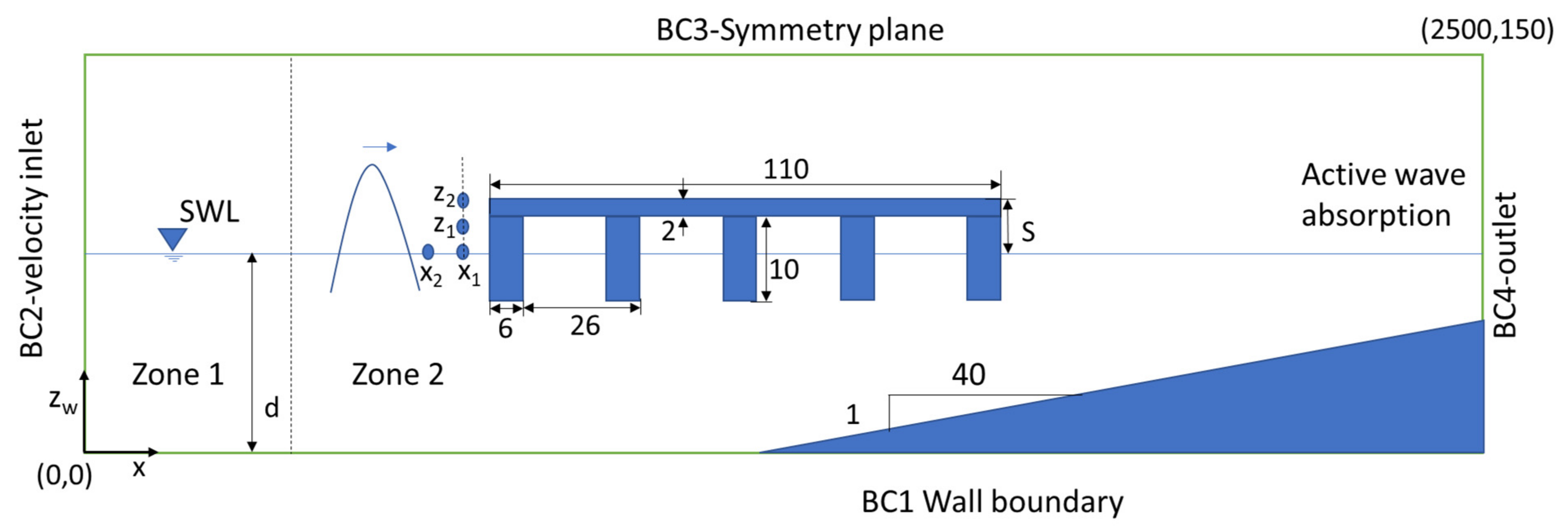
The numerical wave tank modelled was divided into two zones; zone 1 represents the wave generation zone, and zone 2 is the working zone, as shown in Figure 1. The wave generation zone and the working zone are fixed at two and six times the peak wavelength, respectively. The wave generation zone is a relaxation zone, where the velocities and free surface are ramped up to match the wave theory. The active wave absorption method was used at the end of the numerical wave tank to prevent the reflected waves. The initial boundary condition was the velocity inlet with Schaffer’s second order focused wave as input. A symmetry boundary condition was used for the 2D wave tank whereas the bottom has a wall boundary condition. The coastal deck structure has been placed in the working zone for calculating the wave impact forces.
The numerical wave tank used has a length of 25 m, height of 1.5 m with one mesh size as the width. The height and width are maintained same for all the numerical simulations, whereas the length varies with the input peak wave length. The coastal deck structure is scaled down (1:10) to fit into the numerical tank dimensions. The scaling is in accordance with the Froude’s Law. The prototype dimensions considered for the present study are detailed as in Table 1. The significant wave height and peak wave period are given as input and the wave length has been calculated using wave dispersion relationship. The initial wave length reduced with an increase in the wave height as the wave travels along the numerical wave tank. The impact forces obtained are scaled up to the prototype scale and normalized in the presented results. As the simulations are two-dimensional, the results are not highly influenced by the scale [52]. The forces obtained from the two-dimensional simulations are presented as the total force on the entire bridge deck, i.e., they are multiplied by the bridge span length.
The two-phase CFD model (REEF3D) based on the Reynolds-Averaged-Navier–Stokes (RANS) equations coupled with the level set method (LSM) and k-ω turbulence model was used to simulate spilling breakers over a sloping bed using Cnoidal and Solitary waves by [53] Their study validated the numerical model with the experimental data measured by [54]. The model was proven to capture the prominent features such as motion of air pockets in the water, formation of a forward moving jet, the splash up phenomenon and mixing of air and water in the breaking region. The simulated horizontal velocities and free surface elevations are in good agreement with the experimental measurements.
The present section deals with the validation of numerical model for focused wave breaking [31]. The breaking of focused wave groups was carried out for two breaking wave scenarios and the surface elevations are compared. The breaking of focused wave on the deck was numerically simulated and compared with the experimental results of [36] by [55]. Additionally, the present study does not consider the breaking of waves on the shore.
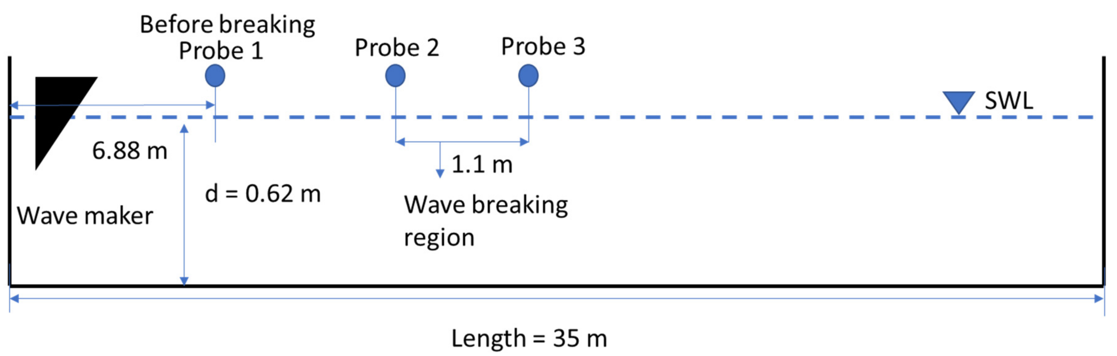
The breaking of wave groups carried out experimentally by [31] was considered a bench mark study for the validation of the numerical model. They simulated the breaking of the wave groups by dispersive wave focusing by specifying constant wave steepness and gain factor. The experiments were carried out in a 2D wave tank with 35 m length, 0.7 m width and 0.62 m water depth (Figure 2). Both breaking and extreme breaking wave groups were generated and the surface elevations were plotted. Two cases of [31] with wave id W4G4 and W5G2 having peak frequencies of 1.025 and 1.245 Hz and constant steepness of 0.669 and 0.483, respectively, were considered in the present validation. The surface elevations during the breaking is recorded by placing three wave gauges (Probe 1, Probe 2 and Probe 3) in the breaking region of the wave tank [31]. The surface elevations are recorded for one upstream and two downstream locations relative to wave breaking. The position of probes is varied depending on the breaking location for different cases considered in the experiment. The breaking scenarios generated for the two cases (W4G4 and W5G2) were considered to validate numerical model REEF3D. The surface elevations are plotted at locations, x = 13.94, 15.7 and 18 m for W4G4 and locations, x = 11.4, 12.59 and 14.73 m for W5G2.
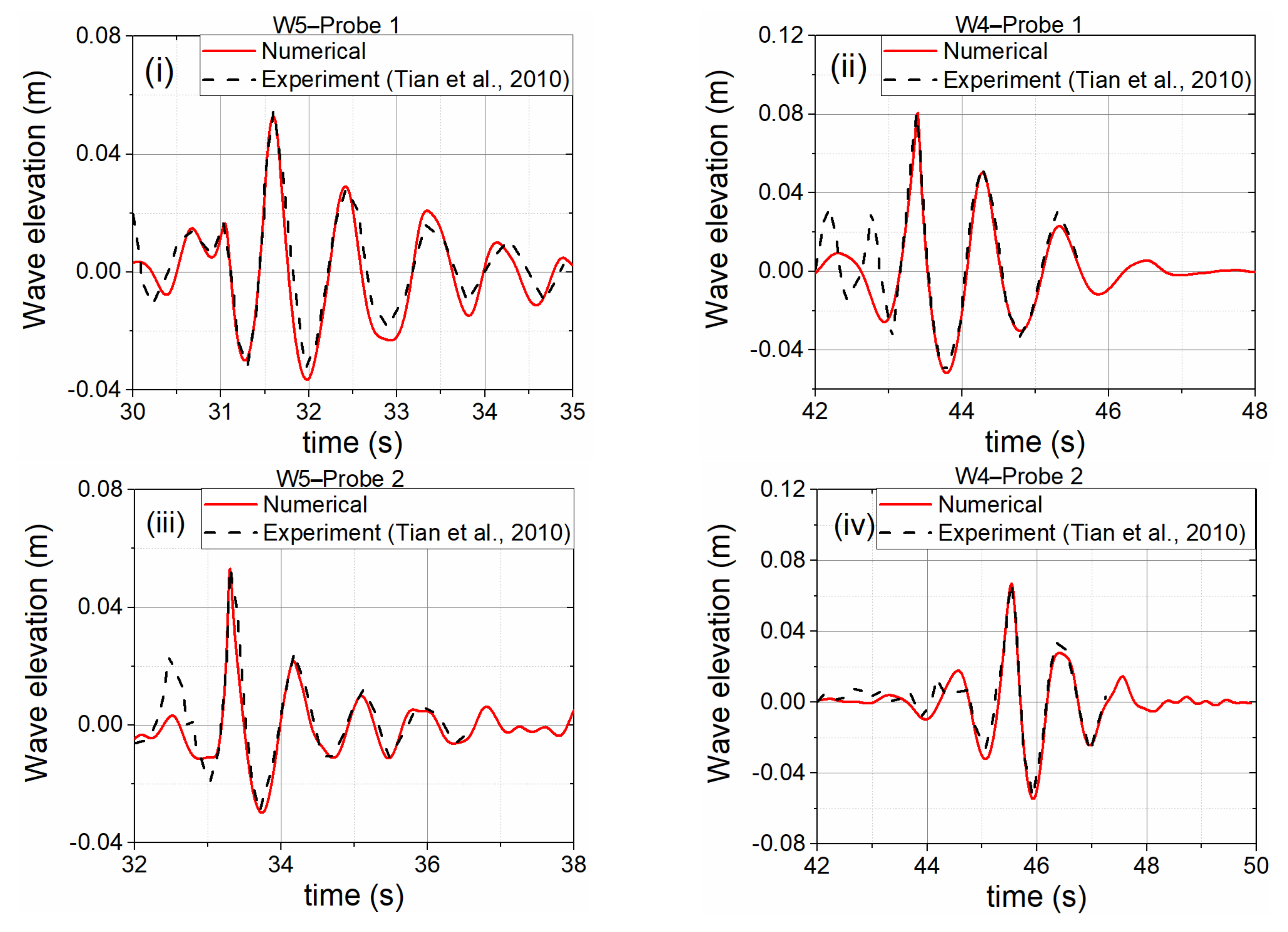
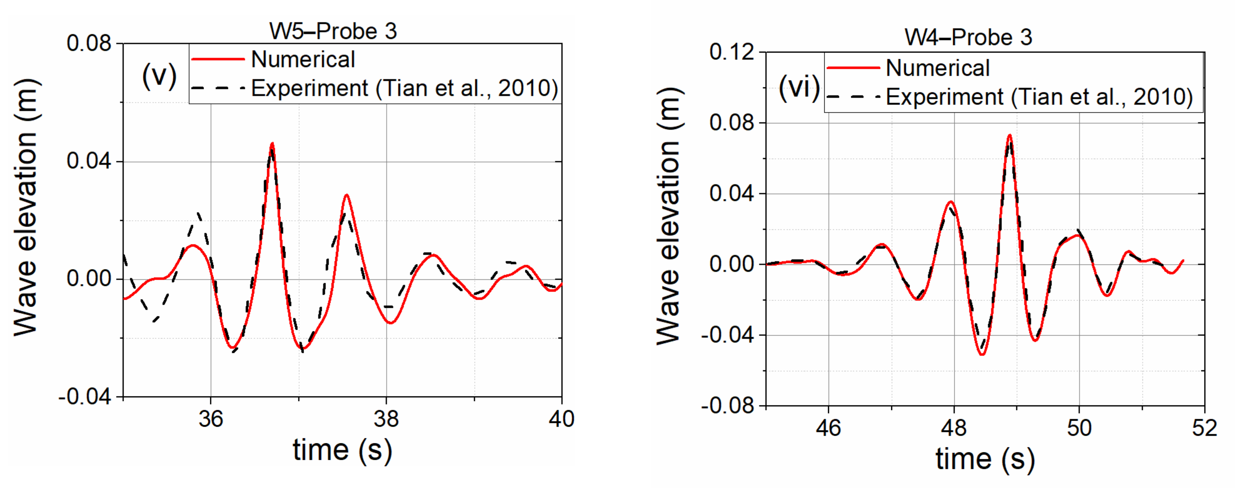
Figure 3 shows the comparison of surface elevation obtained numerically using REEF3D at three probe locations with the experimental results of [31]. The magnitude and phases of surface elevation time history are in good agreement, and the numerical model can be further used for focused wave group breaking studies. The present validation was performed for the breaking focused wave in constant water depth, whereas the simulation using REEF3D of the breaking process in varying water depth forming the spilling and plunging breakers was validated by [53].
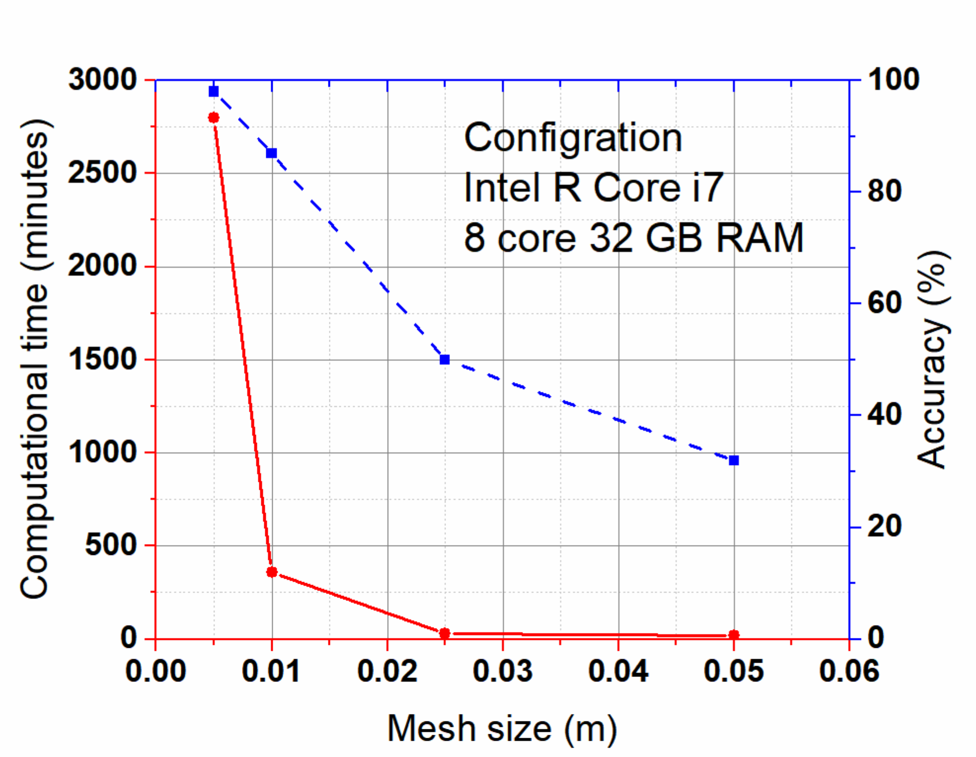
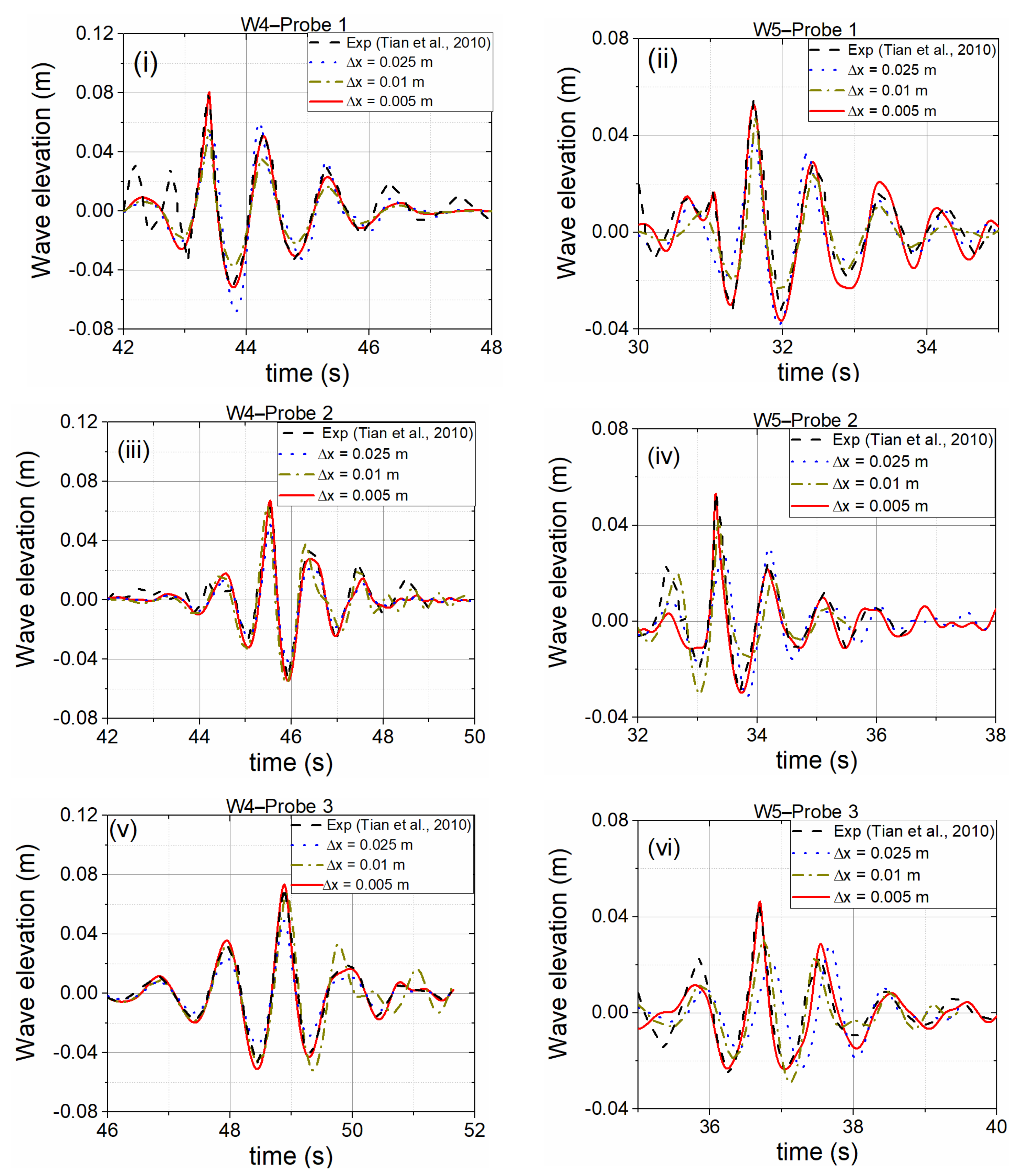
A mesh refinement study was carried out using four different mesh sizes, Δx = 0.005, 0.01, 0.025, and 0.05 m using a desktop workstation in a parallel computing environment. It is observed (Figure 4) that the computational time increases exponentially when the mesh size is reduced from 0.01 to 0.005 m whereas the accuracy increases only by 8 %. Hence, a mesh size of 0.005 m was considered for all further numerical investigations. Figure 5 shows the comparison of wave profiles at different meshes at three probe locations for the two wave ids (W4 and W5) mentioned above. The mesh size of 0.01 and 0.005 m are able to the capture the wave elevation and the phases for the different probe locations. The mesh size of 0.05 m is found to be not suitable for capturing the breaking phenomenon and is not considered further. The relative errors on the peak wave elevation for wave id, W4G4 at three probe locations considering mesh size of 0.005 m are found to be 2.6%, 0.35 % and 1.2%. Similarly, the relative errors for wave id, W5G2 at three probe locations are found to be 2.7%, 0.36% and 1.3%. The errors related to the phase are not investigated further, as the breaking wave characteristics and locations (Section 3.2) are determined prior to locating the structure.
3.2. Breaking Wave Generation in the Numerical Wave Tank
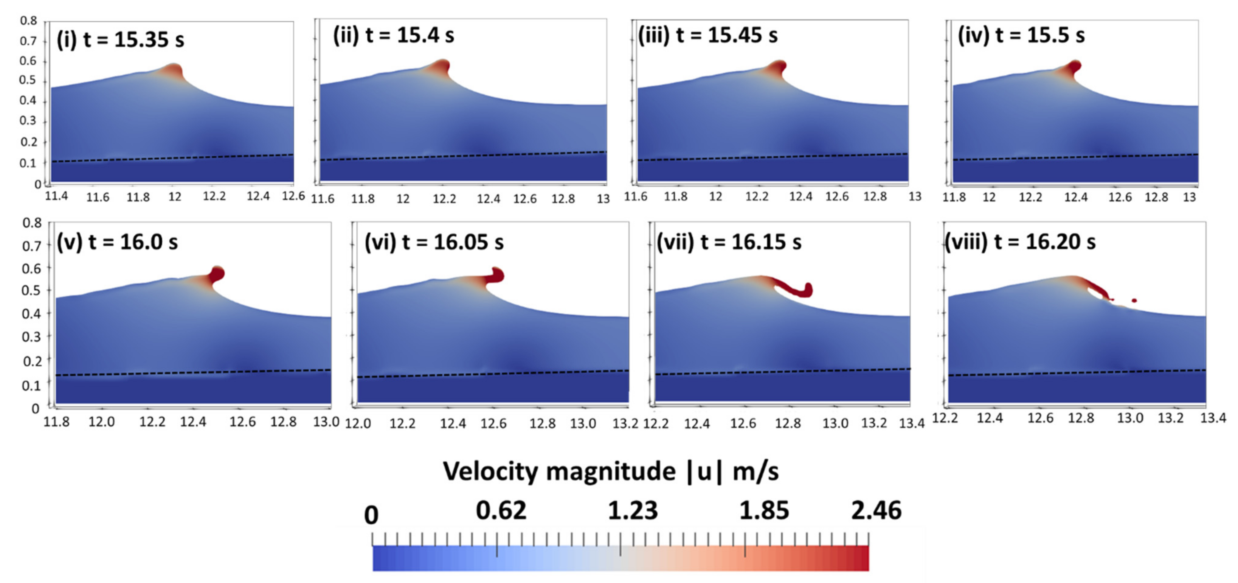
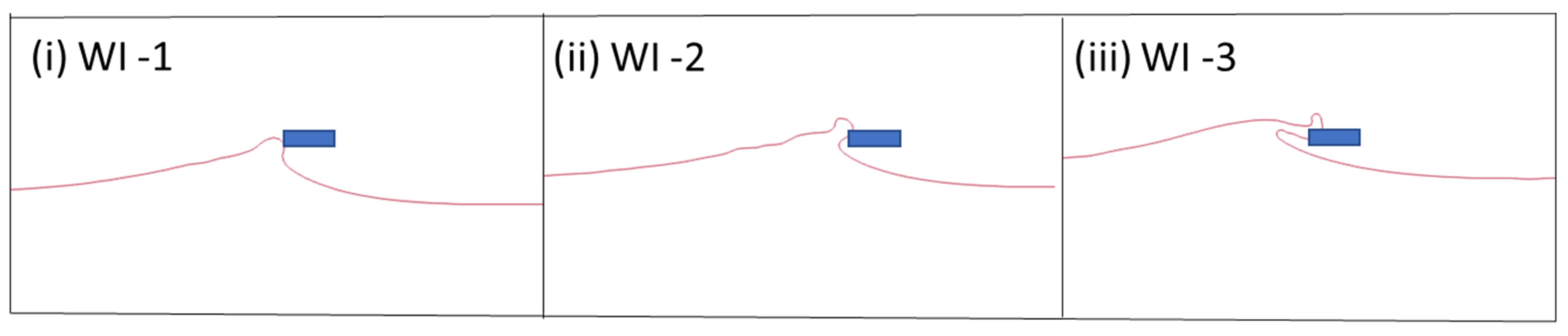
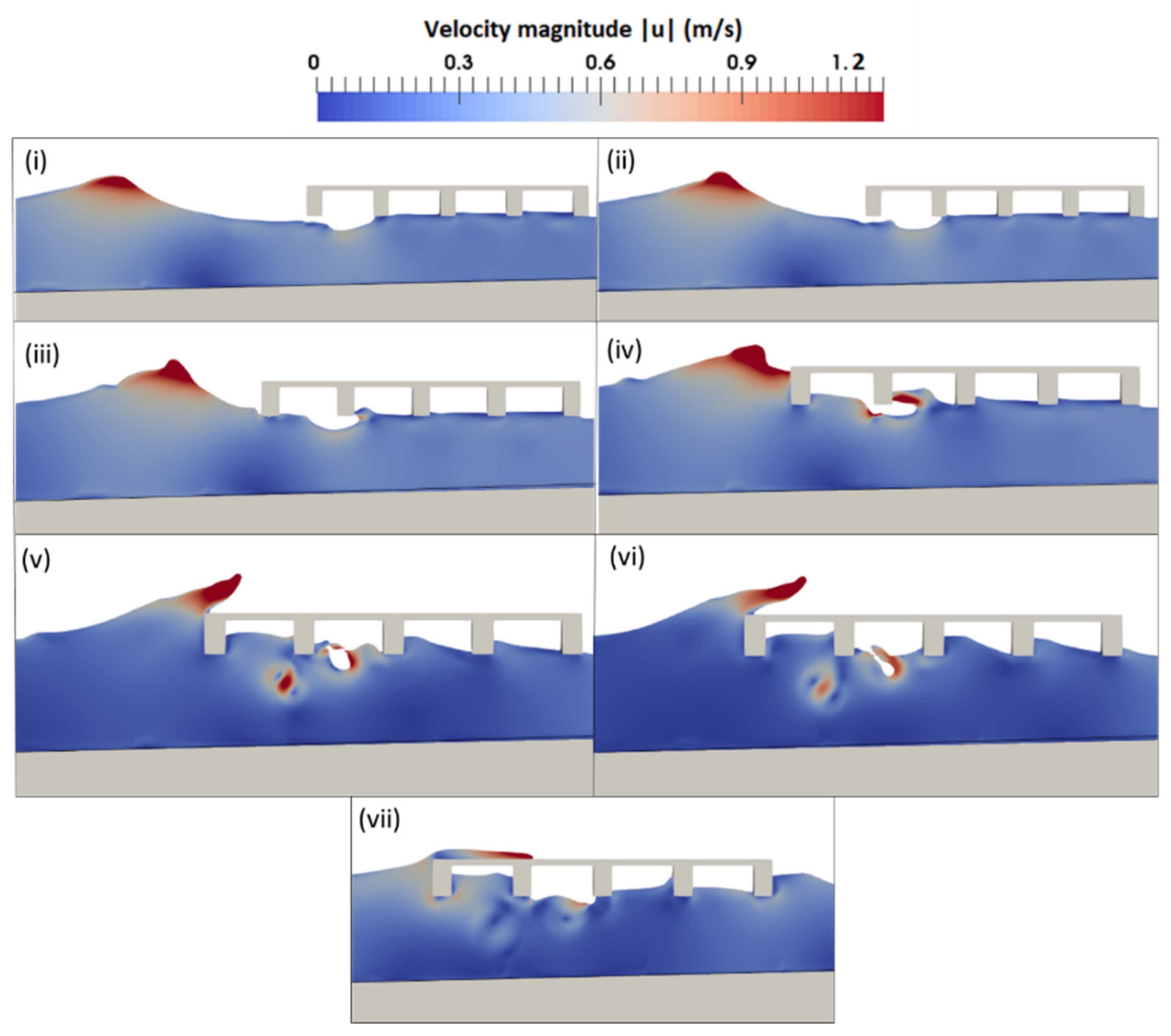
This section demonstrates the numerical wave tank capability for generating breaking waves with varying input conditions. Spilling breakers were generated in the numerical wave tank by breaking high-crested focused waves with larger wave heights on mild slopes. Numerical simulations were carried out in a water depth of 0.45 m for different input significant wave height, peak wave period and mild slopes to generate the breaking condition in the numerical wave tank (as detailed in Table 2). The results are used to select the locations to place the deck structure in order to analyze the effect of breaker location on the impact forces. A surf similarity parameter of less than 0.5 is taken as input to generate spilling breakers. Figure 6 shows the wave breaking process and free surface transformation with velocity magnitude variation at different time steps along the length of the numerical wave tank. These spilling breakers are similar to those obtained by [56]. The focused wave generated travels along the length of the tank and breaks on the slope at larger water depths, whereas the breaking on the shore is not considered here. The symmetrical wave reaches maximum wave height and starts deforming due to shoaling as it rides over the mild slope (Figure 6i,ii). The wave crest becomes vertical with the increase in velocity as the trough depth decreases. As the crest velocity exceeds the celerity, the focused wave crest on the slope overturns (Figure 6iii) with a small-scale jet of water moving forward and hits the trough of the preceding wave (Figure 6viii). The wave crest falling down encloses a pocket of air as it hits the water surface, similar to a plunging breaker. The maximum velocity is seen at the wave crest above the water surface and increases as the wave front propagates, attaining larger steepness. The velocity increases and attains maximum value as the wave crest begins to overturn and plunges to the preceding trough. The wave height increases during the spilling breakers and reaches a maximum of 1.3H0 before breaking (H0 = maximum deep water wave height before breaking starts). The simulations show that the wave height slowly reduces over the mild slopes for the spilling breakers. The reduction indicates that the potential wave energy decreases gradually for the high-crested spilling breakers. Figure 7 shows three breaking wave impact scenarios (WI) occurring over a short time span that are selected for further studies on a coastal deck structure with girders. Wave impact 1 (WI-1) is selected when the wave crest steepens and becomes vertical; WI-2 is the wave impact scenario where the focused wave crest just overturns; WI-3 is the wave impact scenario where the crest plunges before hitting the preceding trough. The location of the three impact events change according to the input significant height, peak wave period and slope.
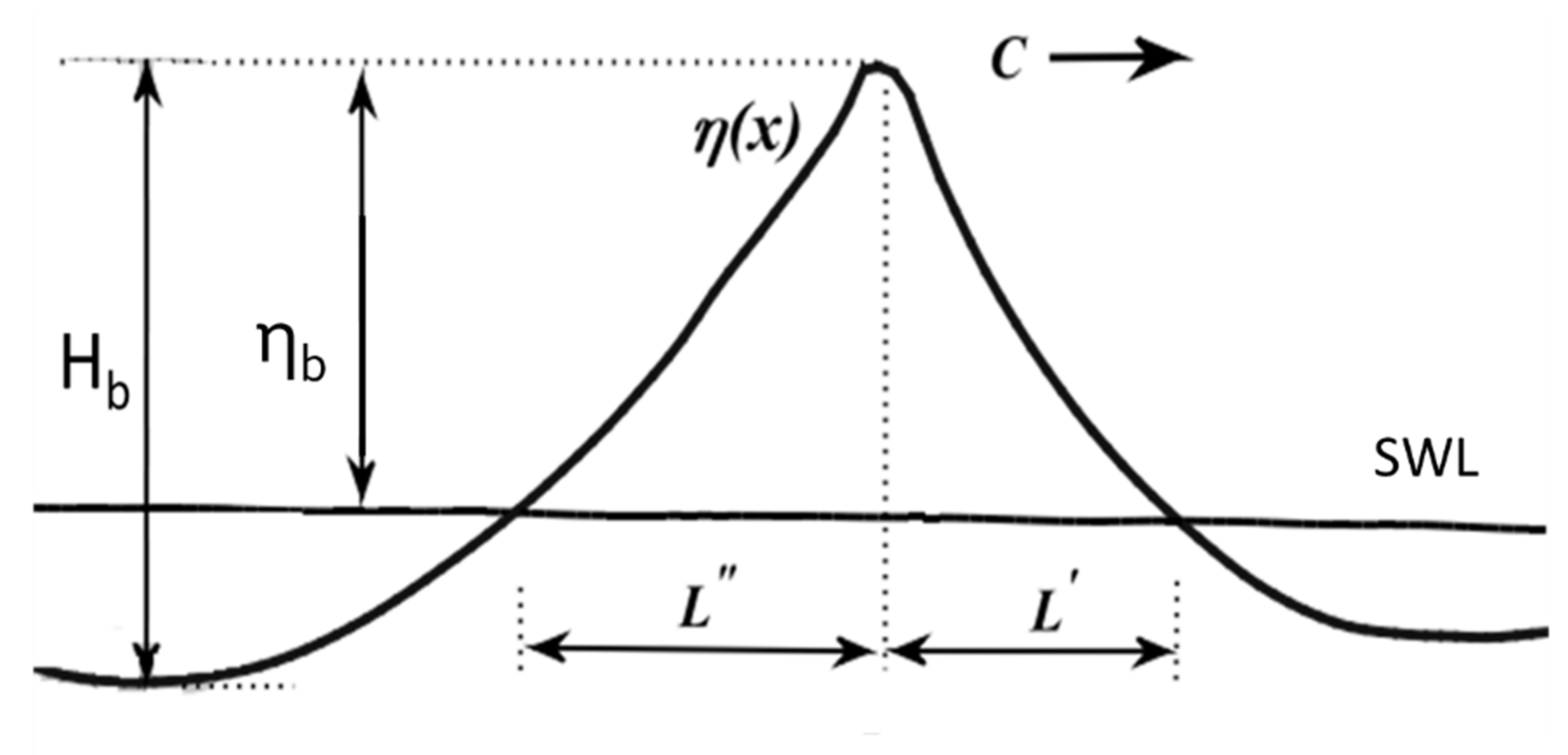
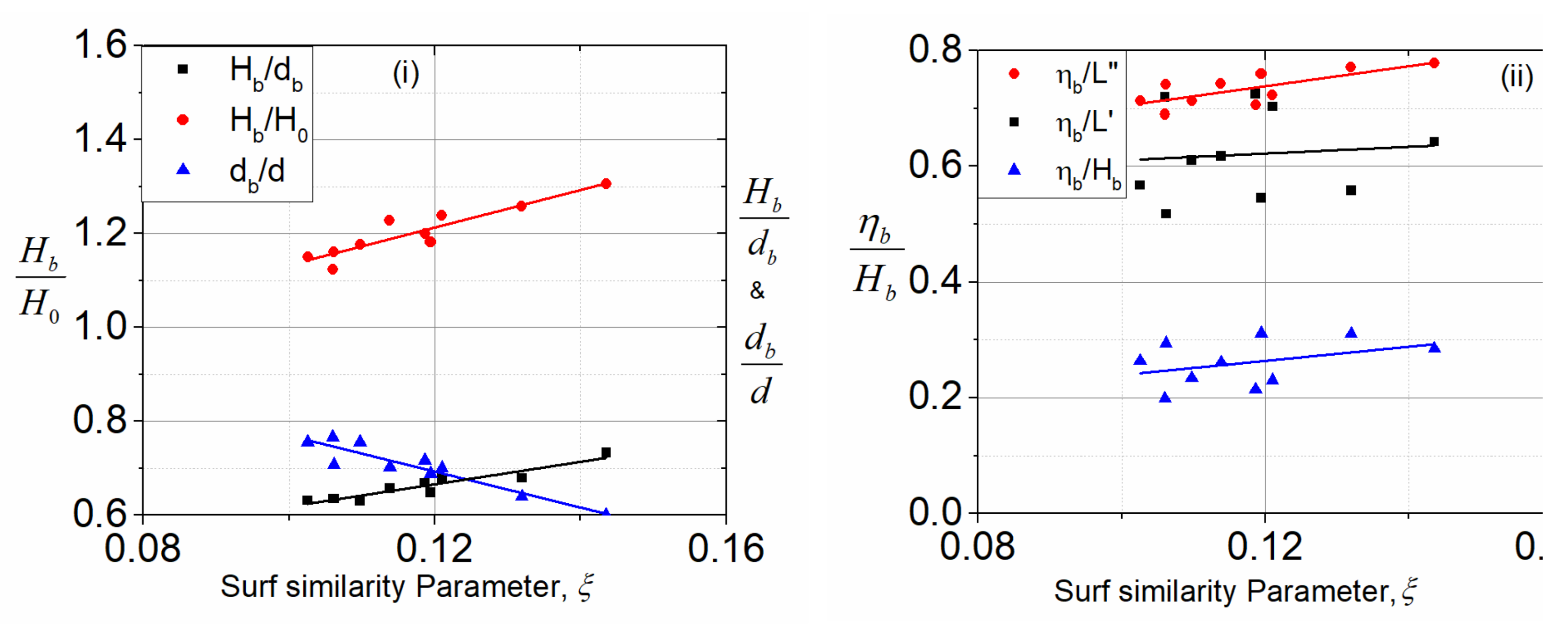
The characteristics and geometry of the breaking waves are analysed and defined based on different breaking parameters given by [19]. Figure 8 shows the breaking focused wave profile and the parameters (ηb, Hb, L′ and L″) taken as per [19]. The characteristics and geometric properties of the breaking waves are defined based on the wave height and water depth at breaking. The slopes are provided in the wave tank based on the surf similarity parameter (), which is a function of seabed slope (m) and deep-water wave steepness (H0/L0). The breaker depth index, breaker height index and relative breaker depth are plotted as shown in Figure 9i with respect to the surf similarity parameter (for different wave steepness, H0/L0 and slopes). The local wave geometry was said to be better represented by other wave parameters such as wave crest front steepness, wave crest rear steepness and horizontal asymmetry factor. Figure 9ii show the above wave parameters varying with wave steepness (H0/L0) and slopes (m). The steepness (ak) of the focused wave also governs the breaking process. The average limiting steepness (ak) obtained for the focused spilling breakers is found to be 0.38, compared to 0.44 for second order Stokes waves in deep water. The study by [20] suggests an average steepness of 0.38 for spilling breakers, while many other researchers also suggested a similar range varying from 0.38 to 0.55.
The relative breaker depth (Figure 9i) shows a decreasing trend with the increase in surf similarity parameter with varying H0/L0 and milder slopes. The possible reason for this is that wave shoaling is higher in mild slopes and the wave breaks faster. As we have considered milder slopes, the wave with higher steepness breaks at higher breaker depth, db. The average value of relative breaker depth (db/d) for different breaking scenarios is 0.7. The breaker depth index (γb) increases with the surf similarity parameter and an average value of 0.65 is seen for different simulations. The breaker height index (Ωb) also shows an increasing trend with the surf similarity parameter with an average of 1.2. The maximum value of breaker depth index, γb and breaker height index, Ωb is obtained for H0/L0 = 0.03 and slope, m = 1/40. It is interesting to note that at this point of offshore wave steepness (H0/L0), db reduces, causing the wave to break at shallower depth (db/d = 0.6). This shows that the waves with higher wave steepness break with higher Hb at milder slopes, resulting in higher values of breaker depth index. Breaker depth index is more influenced by Hb than the breaker depth, whereas breaker height index is dependent mainly on Hb.
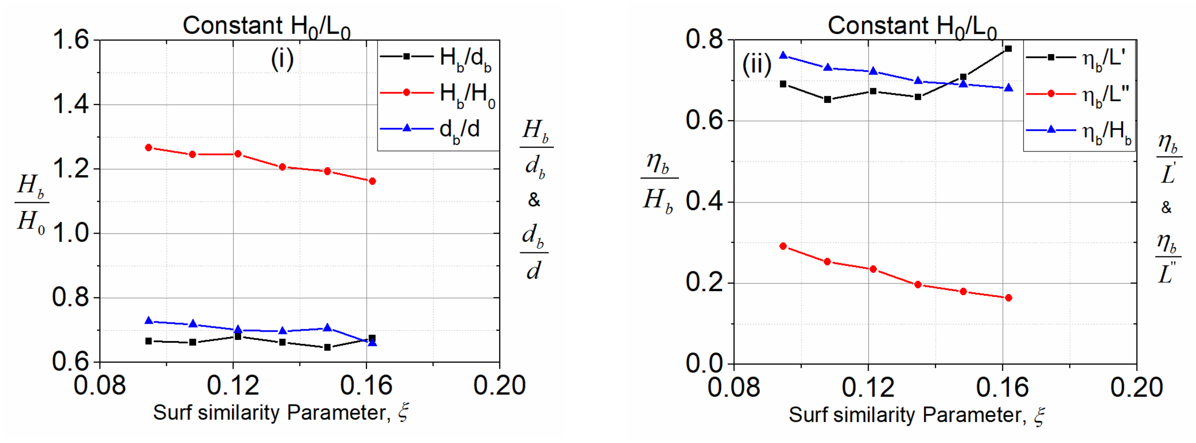
Figure 10i shows the relative breaker depth, breaker height index, breaker depth index varying with the surf similarity parameter for constant H0/L0 (0.035) and varying slopes (1/57, 1/50, 1/44.4, 1/40, 1/36.36, 1/33.33). The results show that the relative breaker depth and breaker depth index are in the range of 0.7 and 0.66, respectively. The average breaker height index is in the range of 1.22, where the index shows a decreasing trend for the values of the surf similarity parameter larger than ξ = 0.12. This shows that the increase in the slope in the range from 0.12 to 0.16 reduces the breaker height, Hb. It is evident that larger breaker height is obtained for milder slopes than steep slopes with higher shoaling and less refection. Additionally, the steeper waves break first at larger water depth whereas the waves with lesser steepness break further onwards at lesser water depths.
The breaking characteristics are better represented by the wave crest front steepness, which is plotted along with wave crest rear steepness and horizontal asymmetry factor for different surf similarity parameters as shown in Figure 10ii (for varying H0/L0 and slope, m). The average wave crest front steepness comes is in the range 0.62, whereas wave crest rear steepness and horizontal asymmetry factor are in the range of 0.26 and 0.73, respectively. The wave crest front and rear steepness is higher for larger wave steepness (H0/L0 = 0.035 to 0.05), whereas the horizontal symmetry factor is higher for lower wave steepness in milder slopes (m = 0.0225 and 0.025). This means that the input wave with larger wave steepness breaks faster with smaller crest and trough deformation whereas the lower steepness waves break with larger deformation of crest and trough with larger overturning crest resembling plunging breakers. Figure 10ii show the variation of parameters (ε, δ, μ) with respect to the surf similarity parameter for constant H0/L0 and varying slope, m. The wave crest front steepness and the horizontal asymmetry factor are in the range of 0.7 and 0.71, respectively. The wave crest rear steepness is in the range of 0.22 for increasing steepness. The wave crest front steepness increases with the seabed slope, whereas wave crest rear steepness and horizontal asymmetry decreases with the seabed slope. This means that the waves undergo more crest deformation and overturning at milder slopes. The breaking waves generated with the above characteristics are further used for studying the impact on decks located at varying airgap positions.
3.3. Breaking Focused Wave Impact on Deck
The breaking focused wave at three impact scenarios (WI-1, WI-2 and WI-3) are forced on a coastal deck structure with girders as shown in Figure 1. The deck structure is modelled to a scale of 1:10 with five girders. The high-crested spilling breaker at three impact scenarios interact with the deck structure, resulting in horizontal and vertical impact forces. The deck is placed at different airgaps (S = 0, 0.02, 0.04, 0.06, 0.08 and 0.1 m) to investigate the interaction of the breaking waves with the structure. Table 3 shows the peak horizontal and vertical impact forces for the different input conditions at three stages of breaking. The db/H0 for different input conditions are also in the same range showing the db changes according to the input wave height. The peak horizontal and vertical impact forces are normalised by the factor , where A can be the horizontal (Ah) and vertical (Av) deck area, respectively.
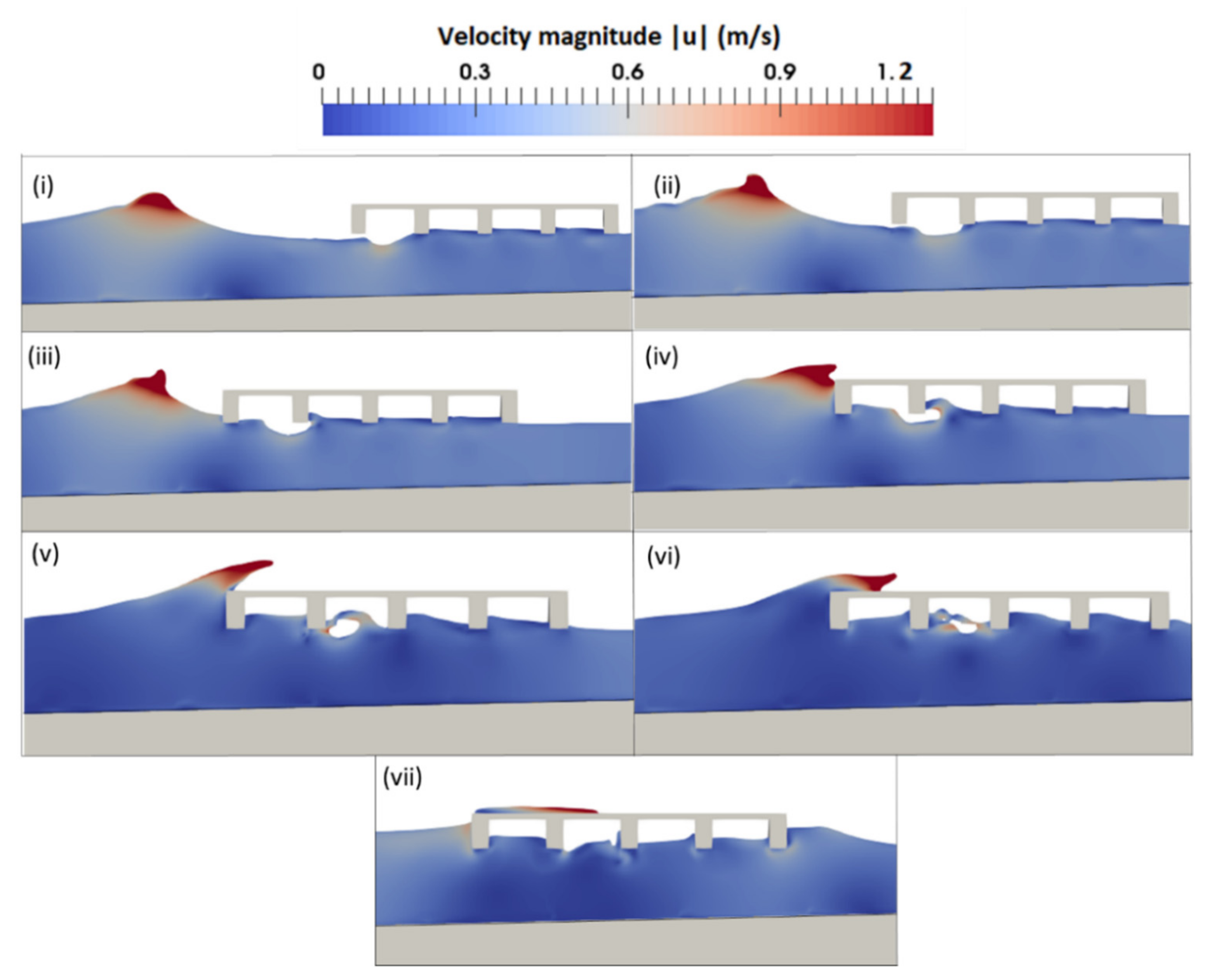
Figure 11 shows the velocity variation during breaking wave impact (Hs = 0.16 m, Tp = 2.5 s) with the deck placed at WI-1 (the first wave impact location where the crest is focused and became vertical). The steep focused wave moving towards the structure (Figure 11i) interact with the girders (Figure 11ii,iii) allowing water to enter the chambers. The wave then hits the deck sides (Figure 11iv) and the wave rises up (Figure 11v). The wave interaction is seen in the first and second chamber with large variation of velocity compared to the other chambers. The wave then hits on top of the deck (Figure 11vi) and water starts leaving the deck and chambers from the trailing edge (Figure 11vii).
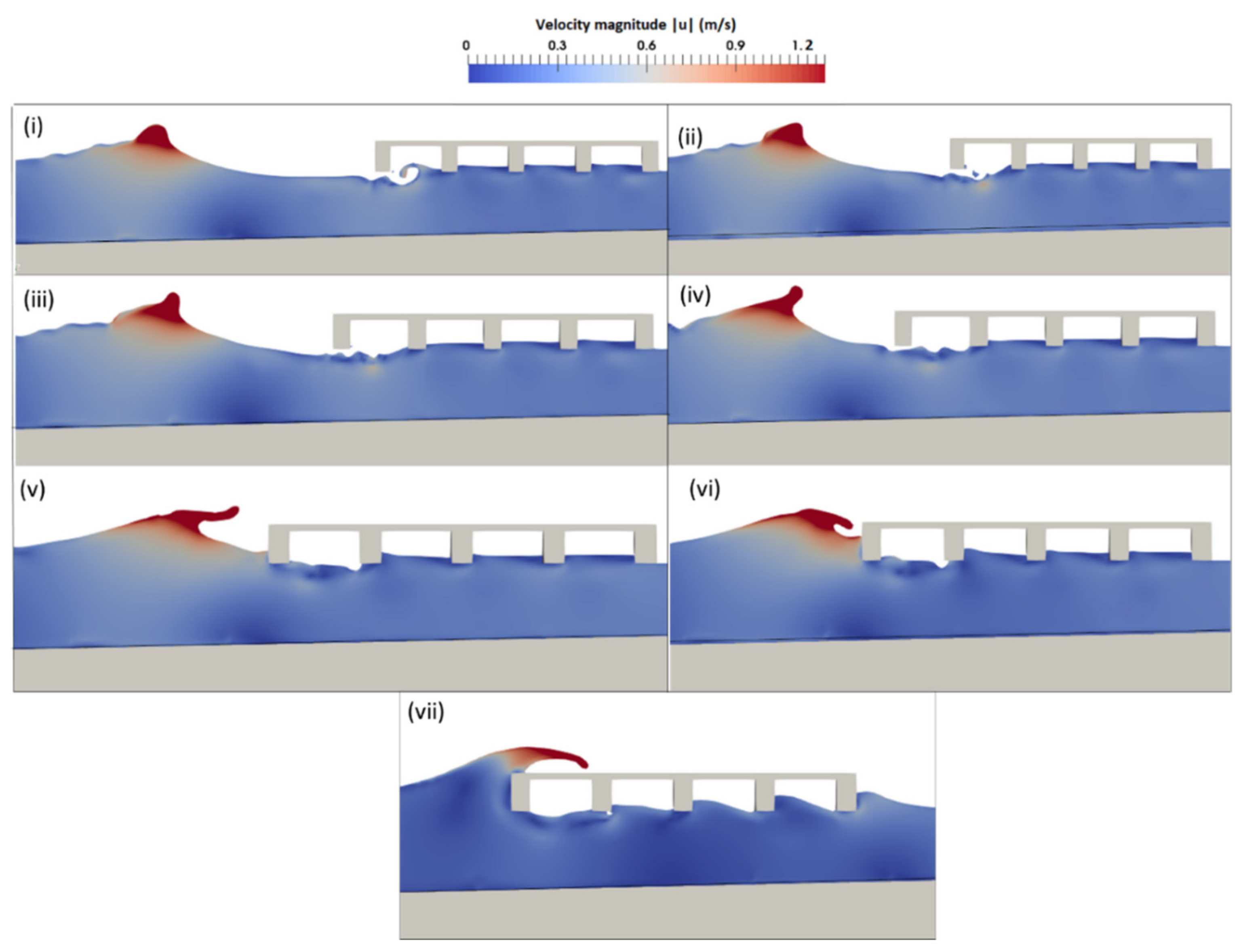
For the second impact scenario, the velocity variation at different time steps along the length of the wave tank is shown in Figure 12. The wave slightly overturns and hits the deck sides with a slight plunge (Figure 12iv). For the third impact scenario, the wave overturns and plunges to hit the deck sides and impact the deck structure (Figure 13). The overturned wave hitting the sides of the deck can be seen in Figure 13iv. For all three impact events, the interaction of the incoming wave with the deck girders occurs before the larger crest hits the deck front. It is observed that the interaction of larger wavelength with the deck bring out changes to the incoming crest before hitting the deck. The breaking events are sequenced for the three impact scenarios (Figure 11, Figure 12 and Figure 13).
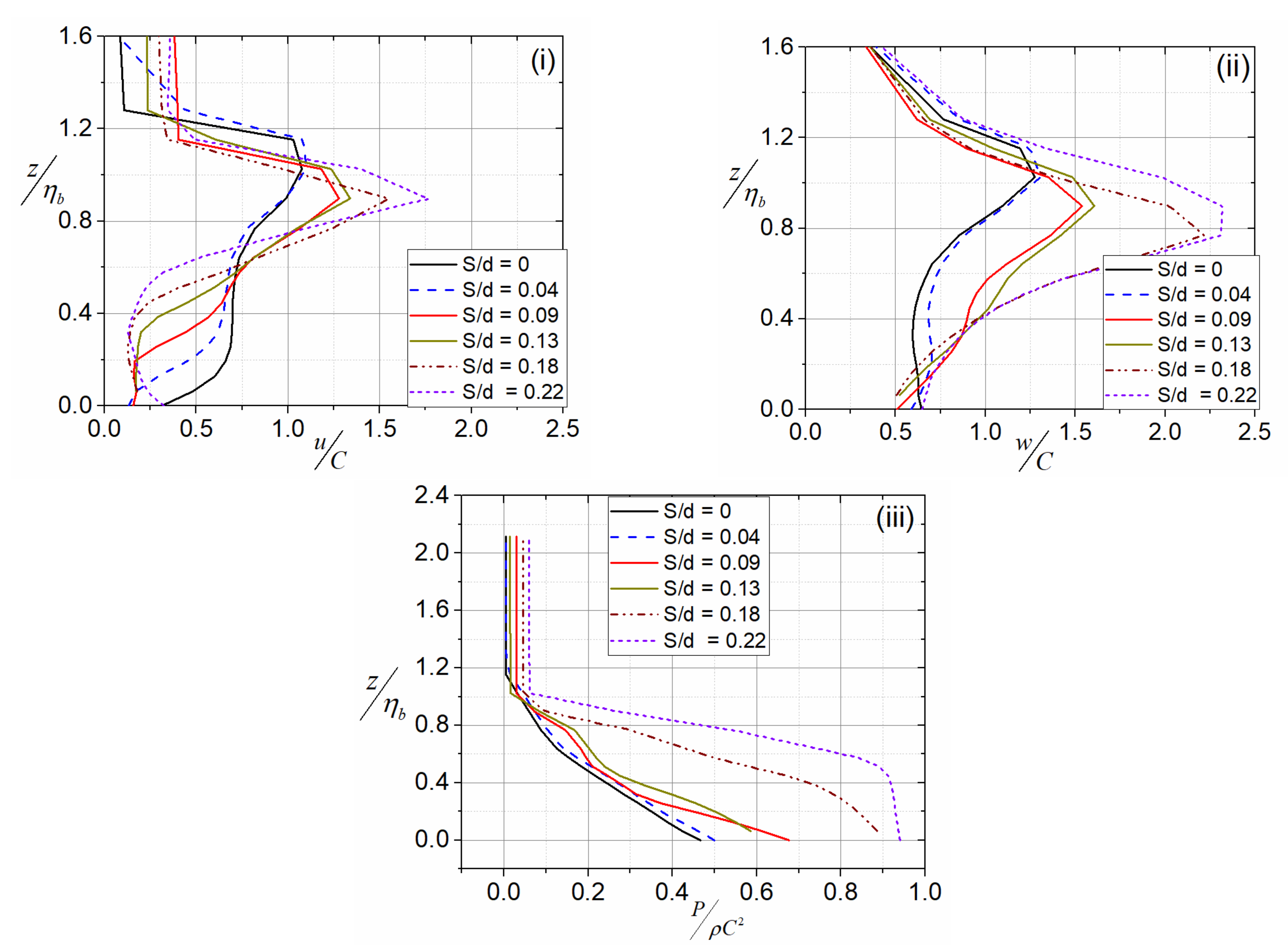
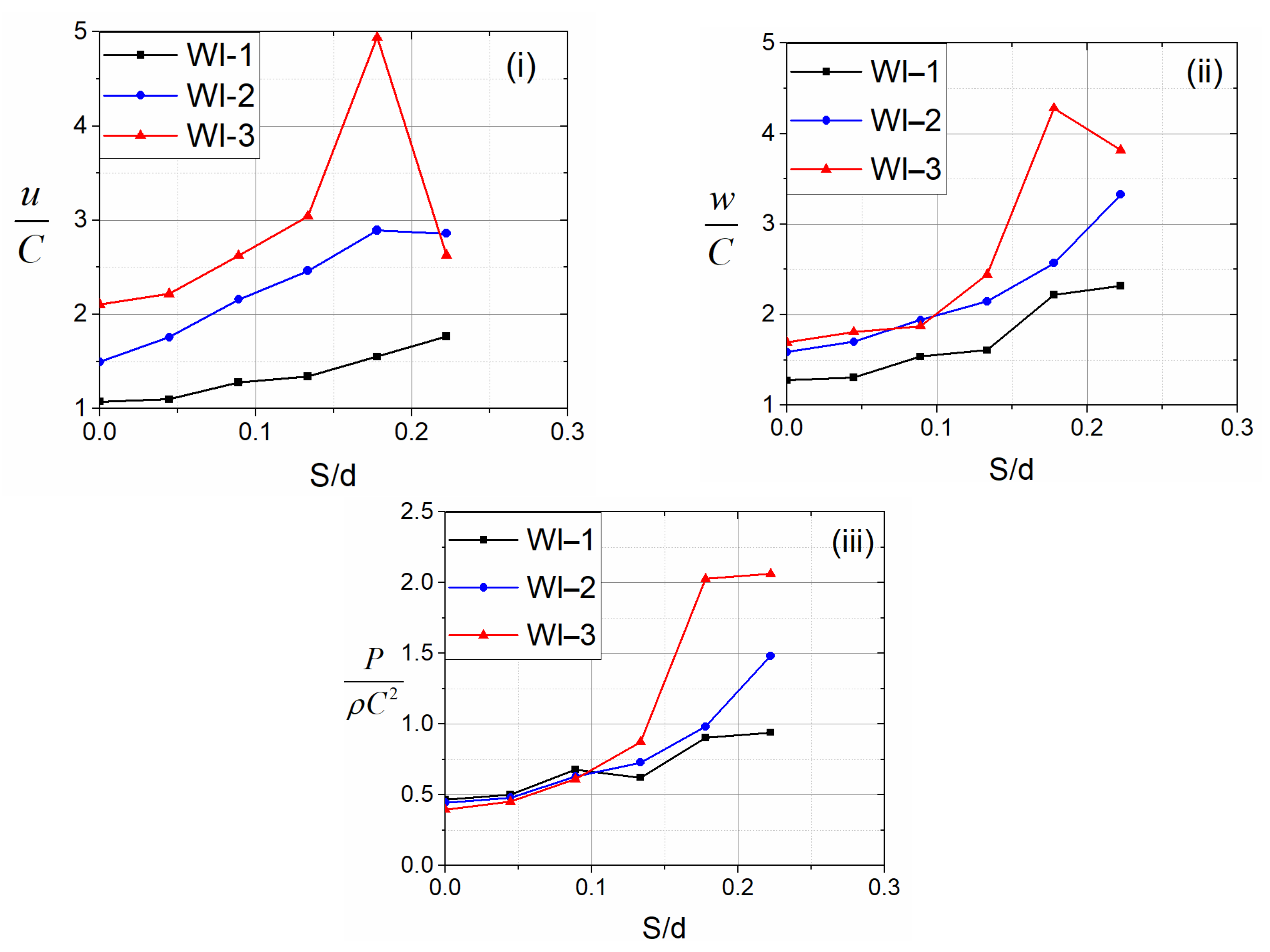
The impact forces on the coastal deck structure varies with respect to the increasing airgap from the still water level. The horizontal velocity (u), vertical velocity (w) and pressure (P) variation along the vertical z-direction of the leading edge of the model (first girder) is plotted. The contribution of three wave impact events to the horizontal force from all the vertical girder surfaces are considered. The maximum values are determined by scanning the distributions over all the vertical surfaces of the structure, which shows that the peak values are at the leading edges of the model. Figure 14 shows the peak variations of velocities and pressure in the vertical z-direction for the first wave impact scenario (WI-1). The velocities are normalised with the corresponding celerity values, whereas the pressure is normalised by the stagnation pressure (ρC2). The vertical axis represents the distance ‘z′ measured from the SWL, which is normalised with the breaking wave amplitude (ηb). Thus, the plots (Figure 14) show the peak values of velocity and pressure above the SWL with respect to the breaking wave amplitude. The normalised peak horizontal and vertical velocity increase with the increase in airgap (S/d = 0.18 and 0.2). The peak values of the velocities are maximum above the SWL, when the z/ηb ratio is nearer to 1. This means the velocities are maximum at the tip of the crest, as is evident from Figure 6. The peak pressure values at the SWL are higher when the structure is placed at higher airgaps (S/d = 0.18 and 0.2, Figure 14iii).
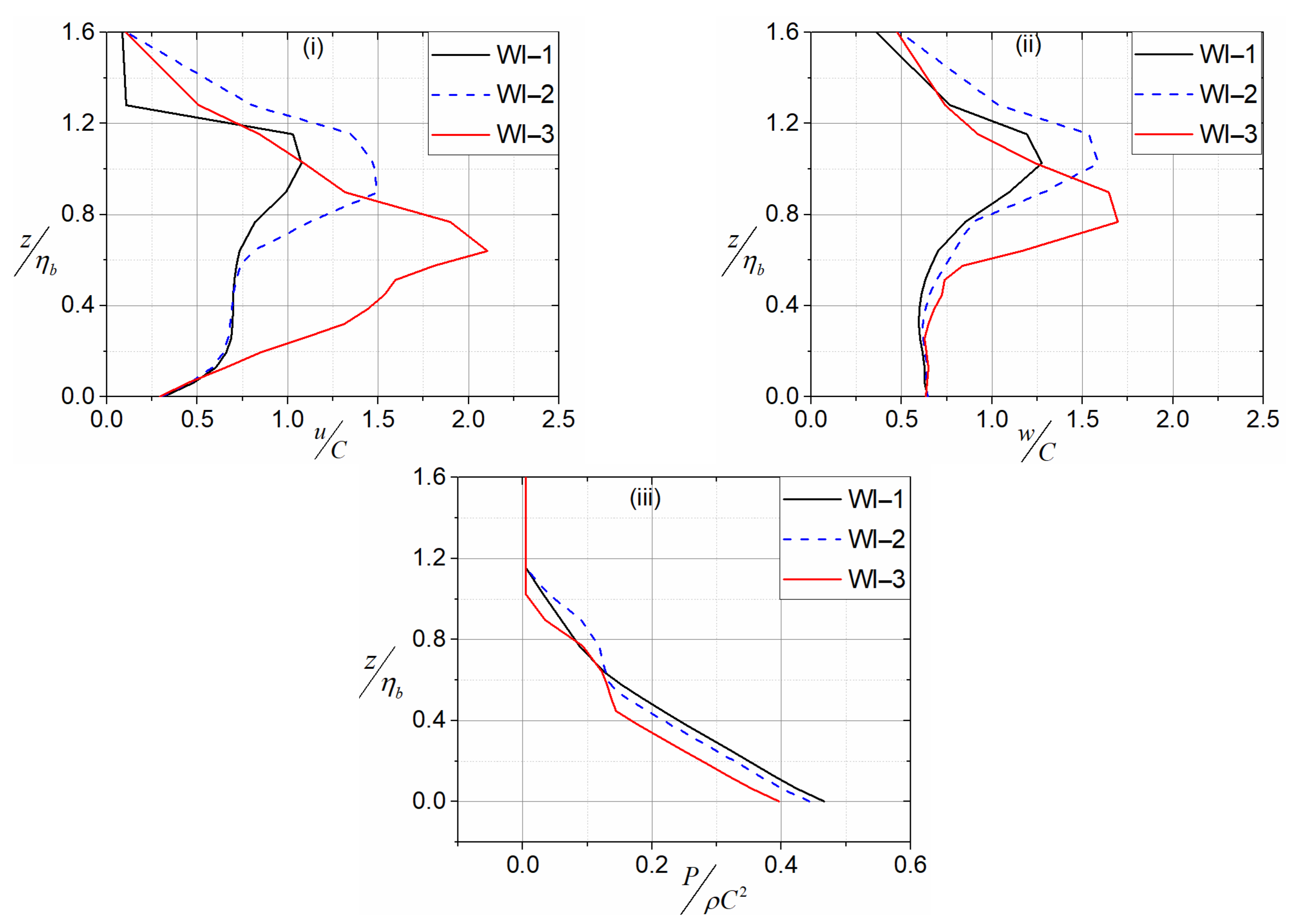
Figure 15 shows a comparison of pressure, vertical and horizontal velocities for the three breaking wave impact scenarios for structure located at SWL (S/d = 0). The vertical and horizontal velocities are maximum for the WI-3 compared to WI-1 and WI-2. The horizontal velocity is higher at z/ηb ratio of 0.6 as the crest plunges, whereas the vertical velocity is higher at z/ηb = 0.8. The pressure is maximum at SWL and varies almost linearly to the top of the breaking wave crest (Figure 15iii). The peak velocities and pressure varying with the increasing normalised airgap, S/d for the three breaking wave impact scenarios are plotted as in Figure 16. The horizontal and vertical velocities (Figure 16i,ii) increase with the increasing normalised airgap, S/d and reduces after reaching the maximum. The particle velocity increases at the wave crest when the water jet grows, moves forward, and plunges the deck located at higher airgap close to the crest. Additionally, the velocity decreases when the structure located above the plunging crest. The peak values of velocities and pressure are also higher for WI-3 compared to WI-2 and WI-1. This increase is because the wave plunges and breaks on the deck for WI-3. The normalised pressure (stagnation pressure) values are higher than 1, which is possible for breaking wave impact conditions (Figure 16iii). The maximum pressure values in the zone of impact are two times higher than ρC2 at higher airgaps. The peak vertical velocity and pressure variation with increase in normalised airgap show a similar pattern for the three wave impact scenarios.
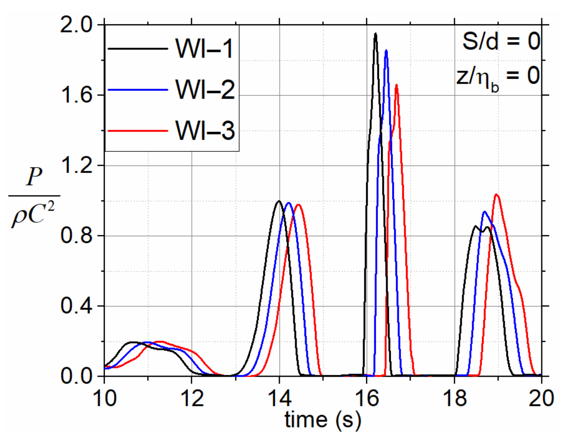
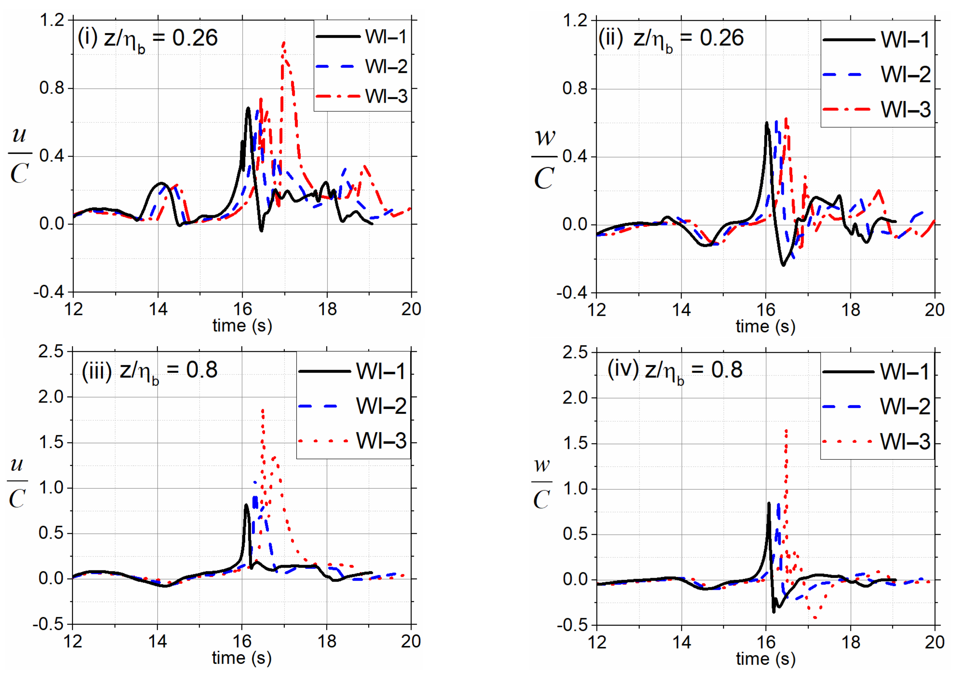
The pressure time history for the three breaking wave impact scenarios at normalised airgap, S/d = 0 is plotted in Figure 17. The maximum pressure is observed for WI-1 compared to the W1-2 and WI-3. The time history of horizontal and vertical velocities for S/d = 0 is also plotted as shown in Figure 18. The normalized horizontal and vertical velocity varying with time at z/ηb = 0.26 (Figure 18i,ii) and z/ηb = 0.8 (Figure 18iii,iv) are plotted. The velocity time history is higher for z/ηb = 0.8 and it occurs within a short time span whereas the velocity time history profile is wider for z/ηb = 0.26. This shows that the velocity profile becomes narrower, and the peak occurs in a short time span as measured above the SWL. The velocity profile becomes wider when the water jet grows faster, and the particle velocity increases as the wave front grows further, narrowing the velocity profile. A portion of the wave crest with higher velocity overturns and impinges the water surface, resulting in a higher peak.
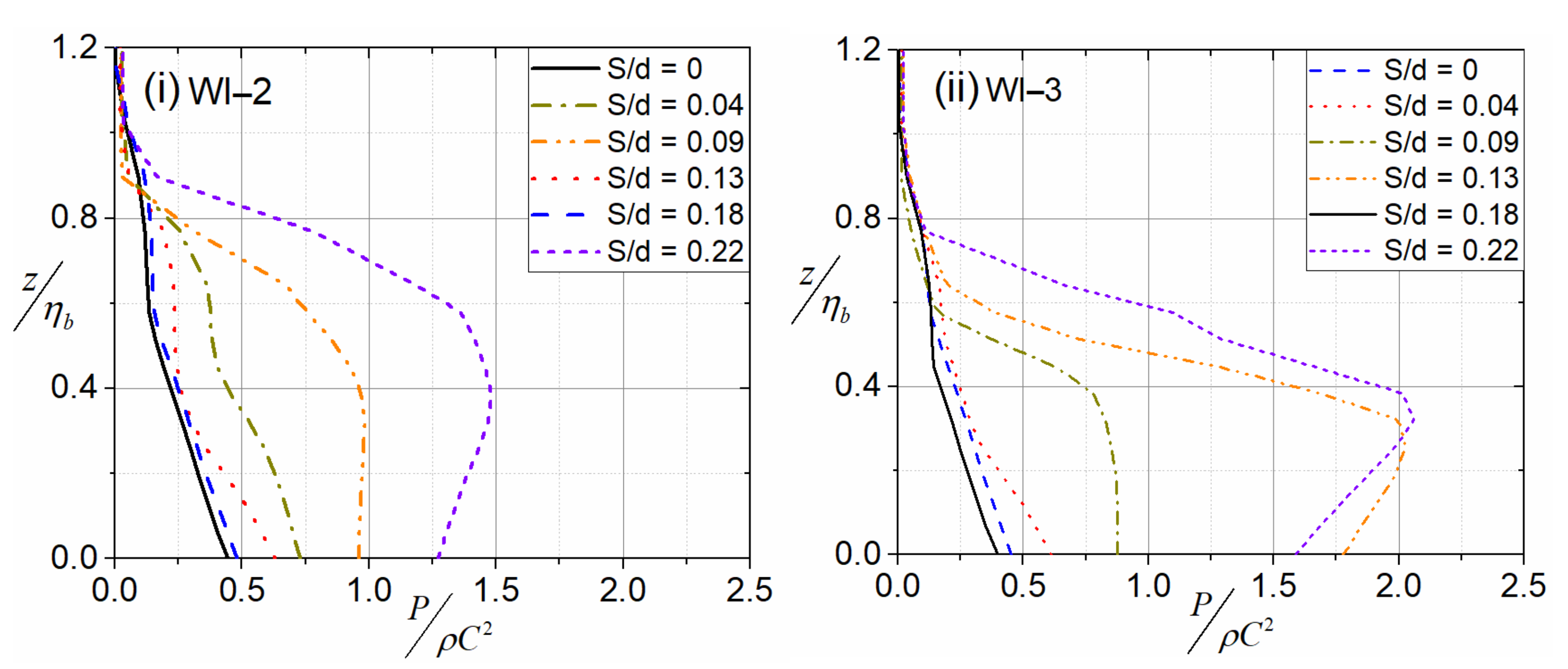
The normalised pressure values are plotted for different airgaps for WI-2 and WI-3 and shown in Figure 19. As the airgap increases, it is seen that the peak pressure is higher above the SWL. This shows that for rectangular objects above SWL, the pressure is found to be higher above the SWL for different stages of wave breaking.
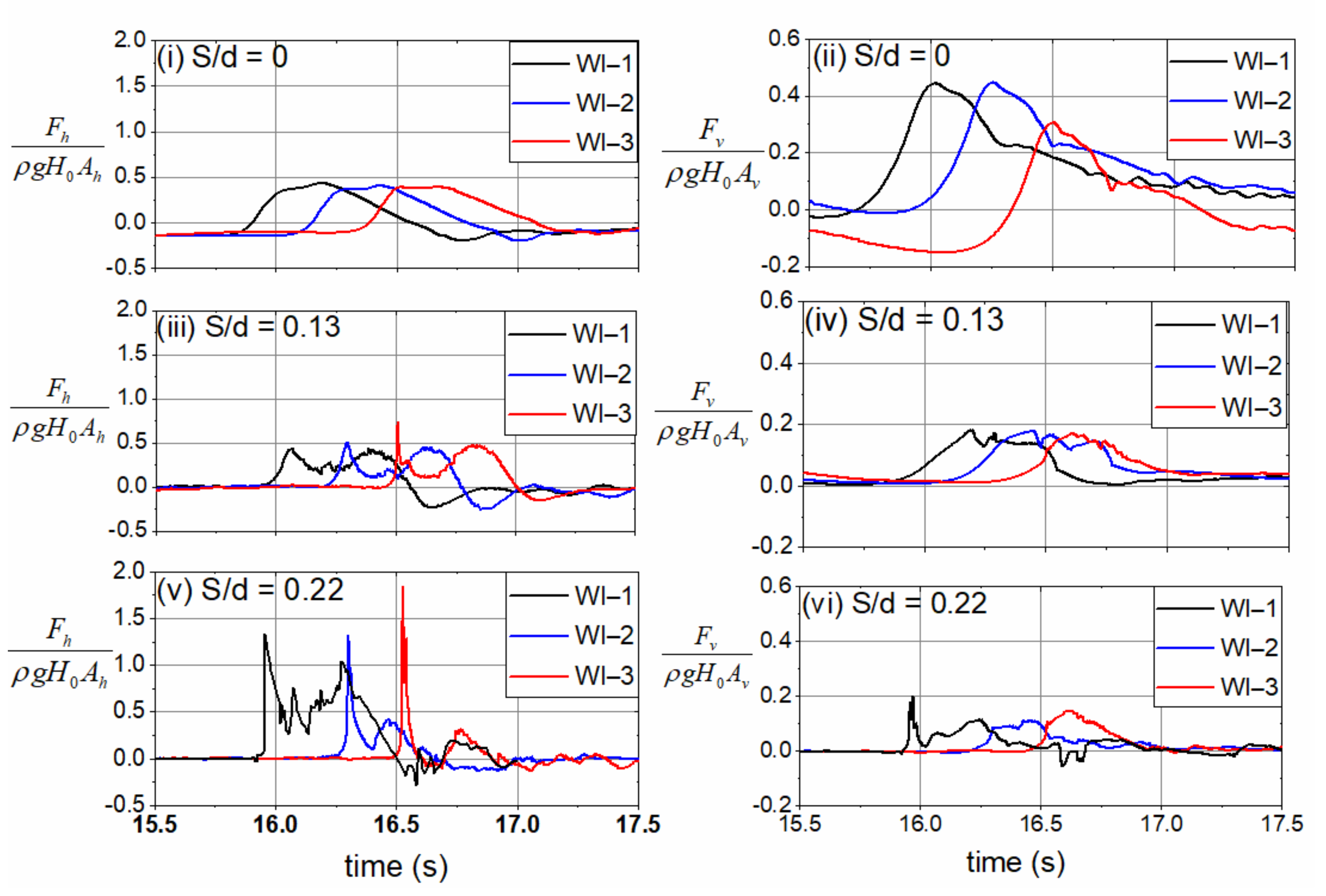
Figure 20 shows the horizontal (Figure 20i,iii,v) and vertical (Figure 20ii,iv,vi) impact force time history at three different increasing airgap positions (S/d = 0, 0.13, 0.22). At zero airgap, the horizontal impact forces for the three impact scenarios are in the same range. As the airgap increases (S/d = 0.13), a peak slamming force is seen in the horizontal force time history for WI-3. With further increase in airgap (S/d = 0.22), a sudden rise is seen in the horizontal force time history for all the impact conditions. The vertical force time history at different airgaps shows a higher peak, when the structure is located at the SWL. The vertical force reduces as the airgap increases. This illustrates that the high-crested spilling breakers imparts higher horizontal impact force at higher airgaps. The short span impulsive force (Figure 21) can induce dynamic fluid structure interaction on the stiff deck structure causing vibrations or large responses. The present study neglects those dynamic behaviour and the structure is considered to be rigid.
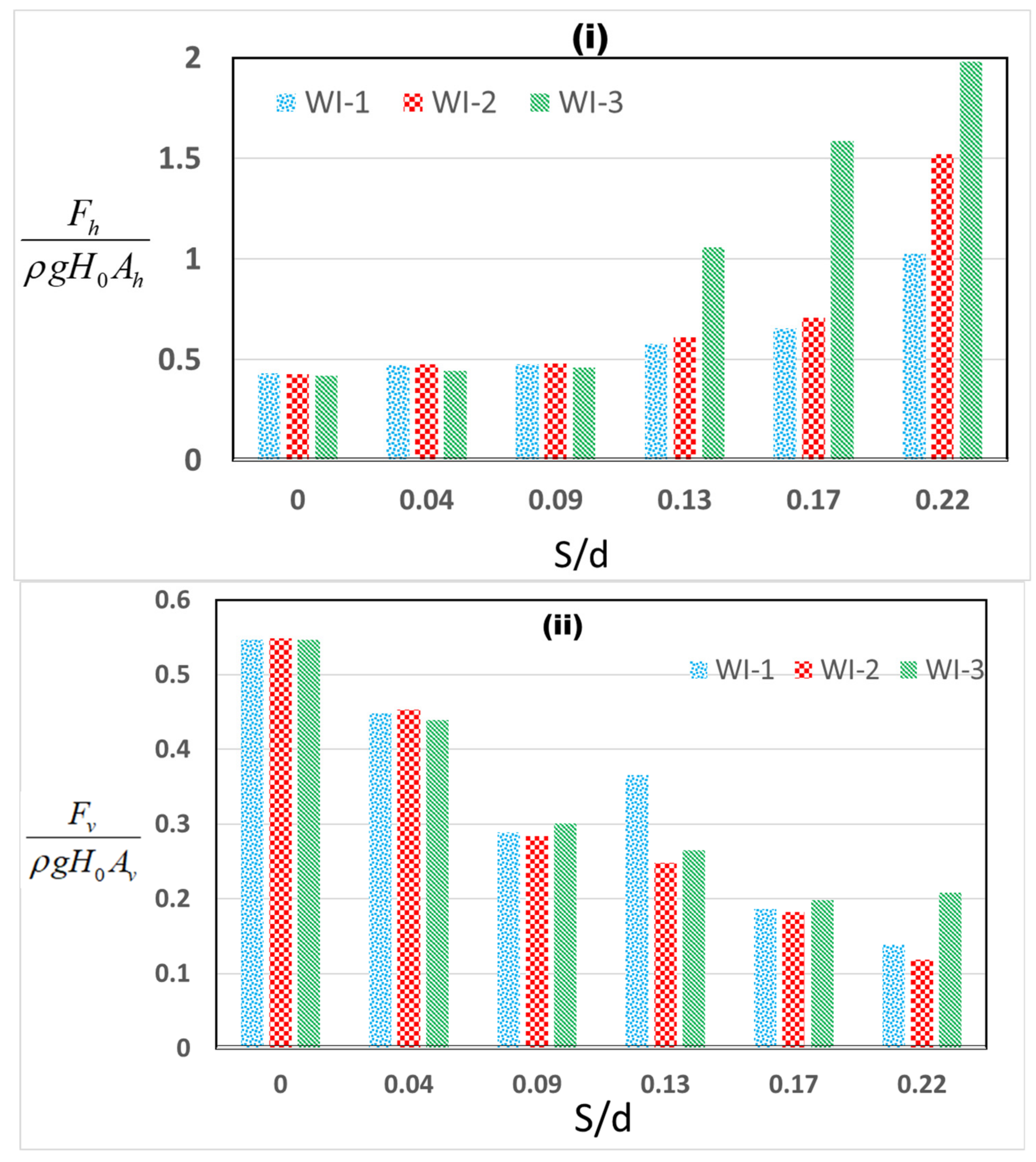
The horizontal and vertical peak impact forces at different airgaps for three breaking wave impact scenarios are shown in Figure 21. The horizontal peak impact force increases with increase in airgap and the maximum value is observed for WI-3. The vertical impact force is maximum at the SWL and then decreases with increase in airgap. The force variation also shows a similar trend as the pressure and velocity profiles.
3.4. Estimation of Force Coefficients Based on Varying Airgap and Wave Height
The present investigation of breaking focused wave impact on deck structures shows that the peak horizontal and vertical impact forces are dependent on both airgap and wave height. The results obtained in the present study are used to derive force coefficients for both horizontal and vertical impact forces based on the Coastal Engineering Manual (CEM). The impact forces are calculated by the reference equation given by the Coastal Engineering Manual [57] for emergent structures, where the force coefficients are derived based on laboratory experiments. The reference equation (given in Equation (11)) is obtained by integrating the pressure over the surface of the emergent structure to compute the forces [58].
where Cu is the laboratory derived coefficient, Az and An are the projected area in horizontal plane and vertical plane, respectively, u and w are horizontal and vertical velocities at level of object, γw is specific weight of water.
The present investigation of breaking focused wave impact on deck structures shows that the peak horizontal and vertical impact forces are dependent on both airgap and wave height. Thus, the constant force coefficients given by the Coastal Engineering Manual (CEM) is not sufficient for computing impact forces on elevated deck structures and requires establishing more suitable coefficients. The results obtained in the present study are used to derive force coefficients for both horizontal and vertical impact forces. The breaking focused wave groups interacting with the deck structure at three impact scenarios (WI-1, WI-2 and WI-3) were considered to investigate the wave structure interaction due to breaking waves. The high-crested spilling breaker at three impact scenarios interact with the deck structure resulting in horizontal and vertical impact forces. The deck is placed at different airgaps (S = 0, 0.02, 0.04, 0.06, 0.08 and 0.1 m) normalised with breaking wave height (Hb) for investigating the interaction of the breaking waves.
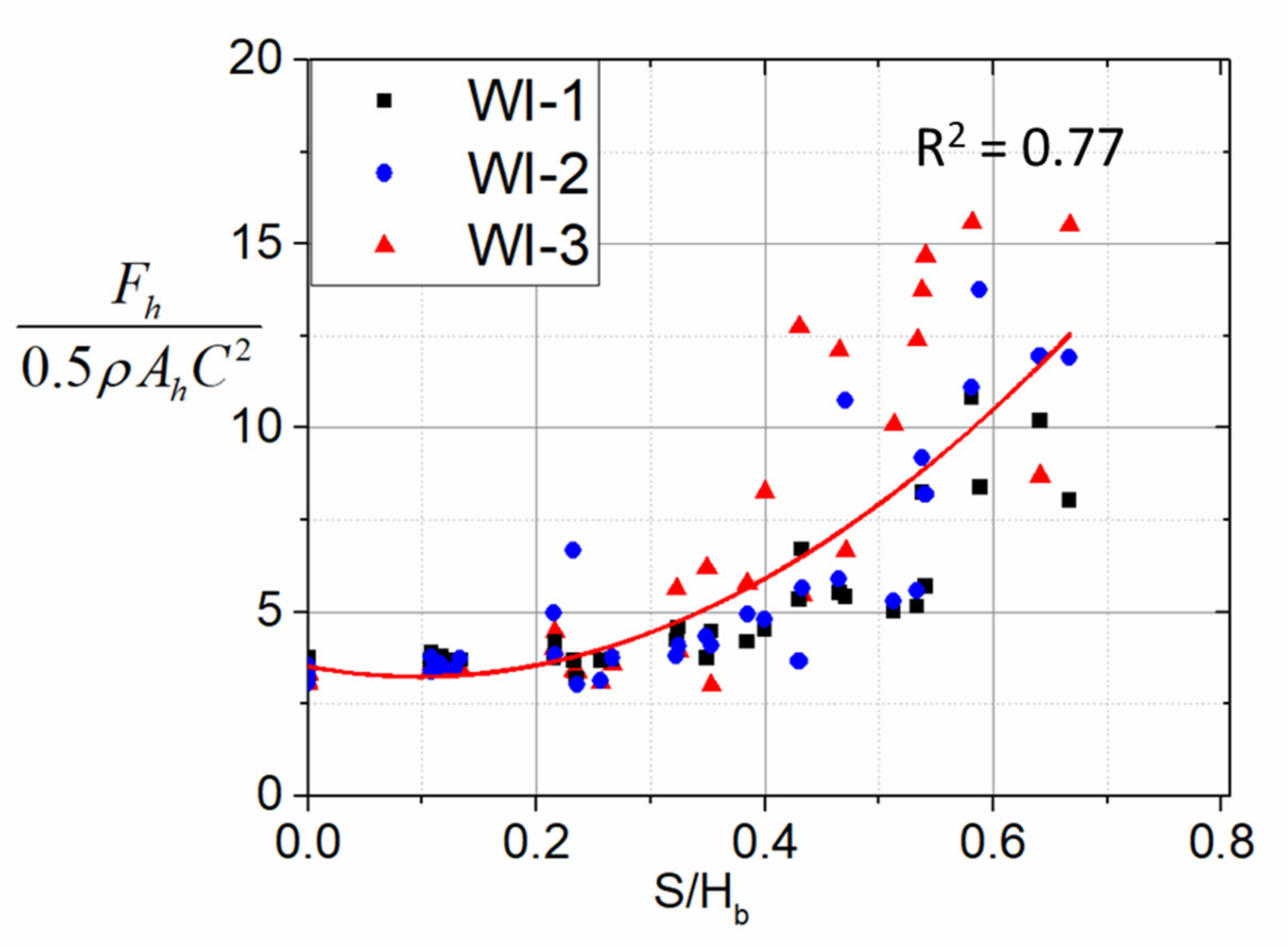
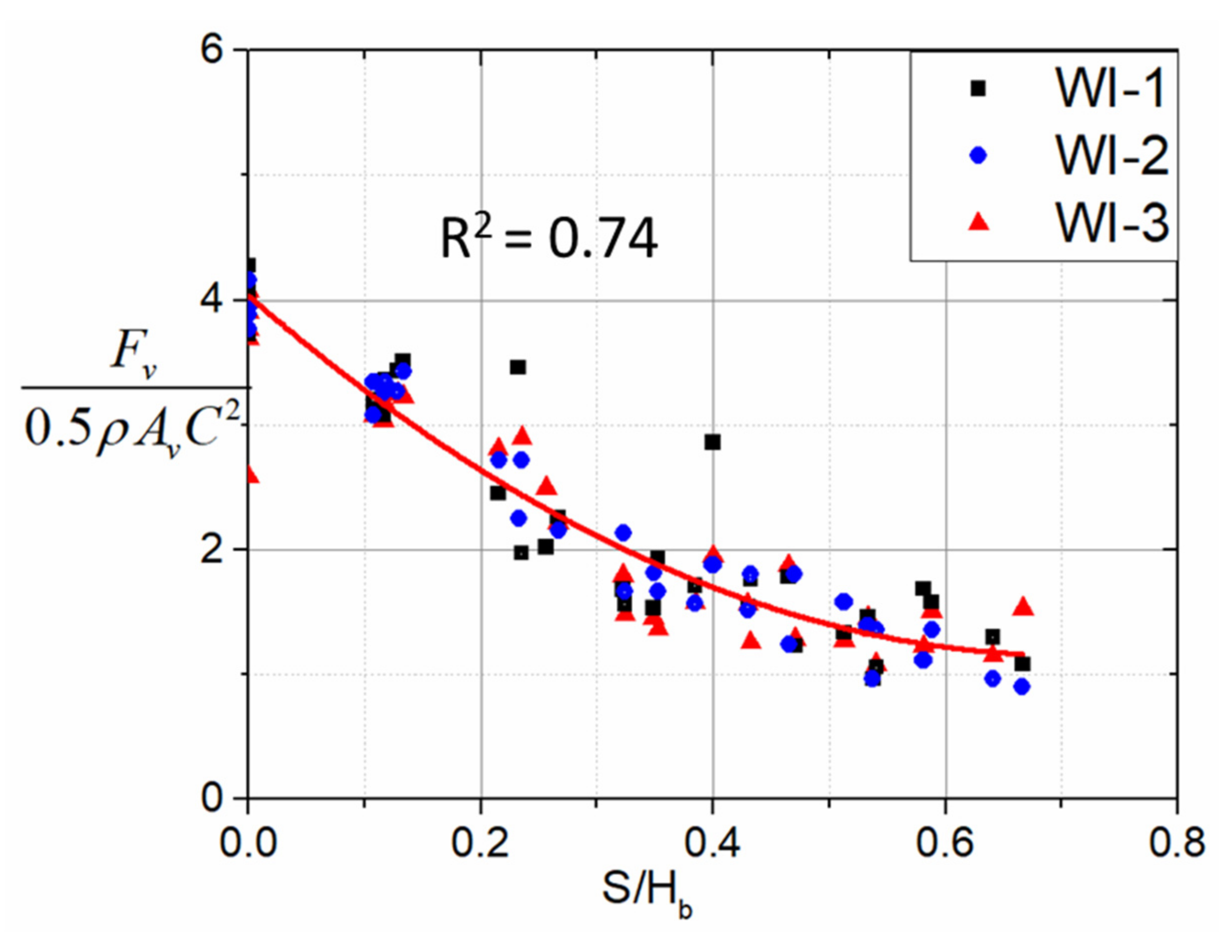
When the wave hits the structure, a sudden change in particle velocities is observed both in the horizontal and vertical directions, making it difficult to choose reference horizontal and vertical velocities to derive the respective coefficients in the practical field. Hence, unlike the CEM reference equation where u & w are used for computing the horizontal and vertical wave forces; wave celerity (C) is used for deriving peak impact force coefficients. The revised formulations for horizontal and vertical force coefficients for breaking wave impact are given as
The variation of force coefficients with respect to varying S/Hb ratios is shown in Figure 22 and Figure 23. Linear regression was carried out for the data sets and best-fit curves representing peak impact forces are plotted. The best-fit polynomials for horizontal and vertical force coefficients for breaking focused wave impact are given in Equations (13) and (14), respectively. The total vertical impact force due to breaking focused wave is the sum of the peak force (Equation (11)) obtained using the modified vertical force coefficients (Equation (14)) and the hydrostatic force due to the surge. The peak horizontal impact force is calculated using the projected vertical area (Av), which is the length of the bridge multiplied by total height of bridge (deck thickness + height of girder). Additionally, the peak vertical impact force is calculated using the horizontal projected area (Ah), which is obtained by multiplying the length of the bridge with the first chamber width (which is the total width divided by number of girders). Only the first chamber width is considered as the peak is obtained when the wave interacts with the first and second girder. The impact forces using the modified coefficients are estimated to predict the peak forces for different wave heights and airgaps.
The relationships between the horizontal and vertical force coefficient with varying airgap and wave height are given as follows:
Horizontal force coefficient (Ch) for breaking focused wave impact on deck structures:
The vertical force coefficients (Cv) for breaking focused wave impact on deck structures:
where S is the airgap measured from SWL to the top of the deck and Hb is the breaking wave height.
The use of the proposed coefficients in the CEM equation is expected to give the peak horizontal and vertical impact force when the high-crested breaking wave hits the deck located at different airgaps. These peak forces are occurring when the wave impacts the first girder or when the wave interacts with the first chamber. Thus, the peak impact forces will depend on the airgap, wave height and the area, Ah and Av. The horizontal projected area takes into account the girder width and spacing whereas the vertical projected area considers the deck thickness and the girder depth. Therefore, the deck thickness, girder depth, deck width, girder width and spacing are considered in the present equations. This makes the modified equations suitable for different structure designs as well.
4. Conclusions
The present study investigated the breaking wave interaction on coastal deck structures at different airgaps on mild slopes using the opensource numerical model REEF3D. The main objective was to investigate the effect of different impact conditions on the pressure, velocity and finally the vertical and horizontal impact forces. Three wave breaking scenarios were considered in the present study where the impact pressure and velocity kinematics are analysed in the vertical direction. Based on the detailed numerical investigations, the following significant conclusions are made:
- The average value of relative water depth for different spilling breaking scenarios of focused wave groups is 0.7 and found increase with the steepness.
- The high-crested focused wave groups generating spilling breakers on mild slopes for different input conditions indicate the breaking wave steepness is approximately 0.38.
- The impact pressure, horizontal and vertical velocities are highest when the overturning wave crest hits the deck. For all impact conditions, the peak impact pressure and velocities increase for the structure located above SWL.
- The peak pressure variation and the horizontal velocity variation are showing similar pattern along the vertical z-direction when the wave breaks and the overturning crest hits the deck located above the SWL.
- As the steep wave front becomes vertical and impacts the structure, the peak horizontal and vertical velocities are near the crest region. As the wave breaks and the crest overturns, the position of the peak velocities moves near to the SWL.
- The breaking wave velocities show significant instantaneous increase near the crest when the breaking wave impacts the deck.
- Maximum impact pressure occurs above the still water level for rectangular objects placed above the SWL under breaking wave impact.
- The peak horizontal impact force is higher when the wave breaks ahead and the overturning wave crest hits the deck positioned above SWL. Additionally, the peak vertical impact force is higher when the deck is placed at the water level. The breaking wave forces on the coastal deck structure are dependent on the breaking impact positions in case of spilling breakers.
- The peak horizontal impact force increases with increasing airgap and follows a parabolic profile with increasing airgap, whereas the peak vertical impact force shows a linear decreasing trend with increasing airgap.
- The force coefficients are derived for peak vertical and horizontal impact forces in relation with varying wave height and airgap for breaking focused wave impact.
This study presented the breaking focused wave characteristics and the impact forces on coastal deck structures with a girder at different airgaps, which provide insight to undertake further studies on breaking wave impact on complex deck structures. The condition for peak vertical and horizontal impact forces due to breaking focused waves was obtained, which will help in assessing damage to the structures. The numerical investigation is performed in a scaled model, which can lead to overestimation of peak forces. The present study neglected the air compressibility, which might play a significant role in modelling air entrapment and the resulting forces. As the breaking scenario is focused, testing the efficiency of different turbulence model can also be carried out. Incorporating the following limitations and comparison with the presented results can give more insight to the breaking phenomenon on decks.
Author Contributions
Conceptualization, R.M. and M.R.B.; methodology, R.M. and M.R.B.; validation, R.M.; formal analysis, R.M.; writing—original draft preparation, R.M.; writing—review and editing, R.M. and M.R.B.; visualization, R.M. and M.R.B.; supervision, M.R.B. All authors have read and agreed to the published version of the manuscript.
Funding
The research received no funding.
Institutional Review Board Statement
Not applicable.
Informed Consent Statement
Not applicable.
Data Availability Statement
The authors confirm that the data supporting the findings of this study are available within the article.
Conflicts of Interest
The authors declare no conflict of interest. The funders had no role in the design of the study; in the collection, analyses, or interpretation of data; in the writing of the manuscript, or in the decision to publish the results.
Nomenclature
| ρ | Fluid density |
| p | Pressure |
| u | Velocity |
| ν | Kinematic viscosity |
| νt | Eddy viscosity |
| g | Acceleration due to gravity |
| k | Turbulent kinetic energy |
| ω | Specific turbulent dissipation rate |
| Pk | Production rate |
| Δt | Time step |
| ε′ | Interface |
| Level set function | |
| H(ϕ) | Heaviside step function |
| Δx, Δy and Δz | Meshes in x, y and z directions |
| η | Instantaneous free surface elevation; |
| (x0, t0) | Predefined focal location and time, respectively |
| k′ | Wave number |
| ω′ | Angular frequency |
| S (fi) | Spectral density |
| mo | Zeroth moment of input spectrum |
| N | Number of wave components |
| A | Target theoretical linear wave amplitude of the focused wave. |
| Tp | Peak wave period |
| Hs | Significant wave height |
| S | Airgap |
| d | Deep water depth |
| ξ | Surf similarity parameter |
| Ωb | Breaker height index |
| γb | Breaker depth index |
| zw | Vertical z direction from origin |
| z | Vertical distance from SWL |
| Cu | Laboratory derived coefficient |
| Ch | Horizontal force coefficient |
| Cv | Vertical force coefficient |
| ε | Wave crest front steepness |
| δ | Wave crest rear steepness |
| μ | Horizontal asymmetry factor |
References
- Chan, E.S. Mechanics of deep water plunging-wave impacts on vertical structures. Coast. Eng. 1994, 22, 115–133. [Google Scholar] [CrossRef]
- Oumeraci, H.; Kortenhaus, A. Analysis of the dynamic response of caisson breakwaters. Coast. Eng. 1994, 22, 159–183. [Google Scholar] [CrossRef]
- Technical Lifelines Council for Earthquake Engineering (TCLEE, 2006). Hurricane Katrina: Performance of transportation systems. In ASCE Technical Council on Lifeline Earthquake Engineering Monograph No. 29, American Society of Civil Engineers, June; Des Roches, R., Ed. Available online: https://ascelibrary.org/doi/book/10.1061/9780784408797 (accessed on 15 March 2022).
- Padgett, J.; Desroches, R.; Nielson, B.; Yashinsky, M.; Kwon, O. Bridge Damage and Repair Costs from Hurricane Katrina Bridge Damage and Repair Costs from Hurricane Katrina. J. Bridge Eng. 2008, 13, 6–14. [Google Scholar] [CrossRef] [Green Version]
- Hansom, J.D.; Switzer, A.D.; Pile, J. Extreme Waves: Causes, Characteristics, and Impact on Coastal Environments and Society. In Coastal and Marine Hazards, Risks, and Disasters; Elsevier: Amsterdam, The Netherlands, 2014; pp. 307–334. [Google Scholar] [CrossRef]
- Seiffert, B.; Hayatdavoodi, M.; Ertekin, R.C. Experiments and computations of solitary-wave forces on a coastal-bridge deck. Part I: Flat Plate. Coast. Eng. 2014, 88, 194–209. [Google Scholar] [CrossRef]
- Hayatdavoodi, M.; Seiffert, B.; Ertekin, R.C. Experiments and computations of solitary-wave forces on a coastal-bridge deck. Part II: Deck with girders. Coast. Eng. 2014, 88, 194–209. [Google Scholar] [CrossRef]
- Azadbakht, M.; Yim, S.C. Effect of trapped air on wave forces on coastal bridge superstructures. J. Ocean Eng. Mar. Energy 2016, 2, 139–158. [Google Scholar] [CrossRef] [Green Version]
- Xu, G.; Cai, C.; Deng, L. Numerical prediction of solitary wave forces on a typical coastal bridge deck with girders. Struct. Infrastruct. Eng. 2017, 2479, 254–272. [Google Scholar] [CrossRef]
- Istrati, D.; Buckle, I.; Lomonaco, P.; Yim, S. Deciphering the tsunami wave impact and associated connection forces in open-girder coastal bridges. J. Mar. Sci. Eng. 2018, 6, 148. [Google Scholar] [CrossRef] [Green Version]
- Moideen, R.; Behera, M.R.; Kamath, A.; Bihs, H. Effect of Girder Spacing and Depth on the Solitary Wave Impact on Coastal Bridge Deck for Di ff erent Airgaps. J. Mar. Sci. Eng. 2019, 7, 140. [Google Scholar] [CrossRef] [Green Version]
- Xiang, T.; Istrati, D. Assessment of extreme wave impact on coastal decks with different geometries via the arbitrary lagrangian-eulerian method. J. Mar. Sci. Eng. 2021, 9, 1342. [Google Scholar] [CrossRef]
- Xiang, T.; Istrati, D.; Yim, S.C.; Buckle, I.G.; Lomonaco, P. Tsunami Loads on a Representative Coastal Bridge Deck: Experimental Study and Validation of Design Equations. J. Waterw. Port. Coastal. Ocean Eng. 2020, 146, 04020022. [Google Scholar] [CrossRef]
- Whittaker, C.N.; Raby, A.C.; Fitzgerald, C.J.; Taylor, P.H. The average shape of large waves in the coastal zone. Coast. Eng. 2016, 114, 253–264. [Google Scholar] [CrossRef] [Green Version]
- Moideen, R.; Behera, M.R.; Kamath, A.; Bihs, H. Numerical modelling of solitary and focused wave forces on coastal-bridge deck. Coast. Eng. Proc. 2018, 36, 12. [Google Scholar] [CrossRef]
- Alagan Chella, M.; Bihs, H.; Myrhaug, D.; Muskulus, M. Breaking solitary waves and breaking wave forces on a vertically mounted slender cylinder over an impermeable sloping seabed. J. Ocean Eng. Mar. Energy 2017, 3, 1–19. [Google Scholar] [CrossRef]
- Aggarwal, A.; Bihs, H.; Myrhaug, D.; Chella, M.A. Characteristics of breaking irregular wave forces on a monopile. Appl. Ocean Res. 2019, 90, 101846. [Google Scholar] [CrossRef]
- Ramberg, S.E.; Griffin, O.M. Laboratory study of steep and breaking deep water waves. J. Waterw. Port Coast. Ocean Eng. 1987, 113, 493–506. [Google Scholar] [CrossRef] [Green Version]
- Kjeldsen, S.P.; Myrhaug, D. Kinematics and Dynamics of Breaking waves. In Rep. No. STF60 A79044, Ships Rough Seas, Part 4, Nor. Hydrodyn. Lab.; Vassdrags og Havnelaboratoriet Norway: Trondhei, Norway, 1979. [Google Scholar]
- Bonmarin, P. Geometric properties of deep-water breaking waves. J. Fluid Mech. 1989, 209, 405–433. [Google Scholar] [CrossRef]
- Swift, R.H. Prediction of breaking wave forces on vertical cylinders. Coast. Eng. 1989, 13, 97–116. [Google Scholar] [CrossRef]
- Zhou, D.; Chan, E.S.; Melville, W.K. Wave impact pressures on vertical cylinders. Appl. Ocean Res. 1991, 13, 220–234. [Google Scholar] [CrossRef]
- Wienke, J.; Oumeraci, H. Breaking wave impact force on a vertical and inclined slender pile—Theoretical and large-scale model investigations. Coast. Eng. 2005, 52, 435–462. [Google Scholar] [CrossRef]
- Tromans, P.S.; Anaturk, A.R.; Hagemeijer, A. A new model for the kinematics of large ocean waves-application as a design wave. In Proceedings of the 1st International Offshore and Polar Engineering Conference, Edinburgh, UK, 11–16 August 1991; pp. 64–71. [Google Scholar]
- Ning, D.Z.; Zang, J.; Liu, S.X.; Eatock Taylor, R.; Teng, B.; Taylor, P.H. Free-surface evolution and wave kinematics for nonlinear uni-directional focused wave groups. Ocean Eng. 2009, 36, 1226–1243. [Google Scholar] [CrossRef]
- Rapp, R.; Melville, W.K. Laboratory measurements of deep-water breaking waves. Math. Phys. Sci. 1990, 331, 735–808. [Google Scholar]
- Kway, J.H.L.; Loh, Y.S.; Chan, E.S. Laboratory study of deep-water breaking waves. Ocean Eng. 1998, 25, 657–676. [Google Scholar] [CrossRef]
- Kharif, C.; Pelinovsky, E. Physical mechanisms of the rogue wave phenomenon. Eur. J. Mech. B/Fluids 2003, 22, 603–634. [Google Scholar] [CrossRef] [Green Version]
- Perlin, M.; Choi, W.; Tian, Z. Breaking Waves in Deep and Intermediate Waters. Annu. Rev. Fluid Mech. 2013, 45, 115–145. [Google Scholar] [CrossRef] [Green Version]
- Tian, Z.; Perlin, M.; Choi, W. Energy dissipation in two-dimensional unsteady plunging breakers and an eddy viscosity model. J. Fluid Mech. 2010, 655, 217–257. [Google Scholar] [CrossRef] [Green Version]
- Tian, Z.; Perlin, M.; Choi, W. Evaluation of a deep-water wave breaking criterion. Phys. Fluids 2008, 20, 066604. [Google Scholar] [CrossRef]
- Bredmose, H.; Jacobsen, N.G. Breaking Wave Impacts on Offshore Wind Turbine Foundations: Focused Wave Groups and CFD. In Proceedings of the ASME 2010 29th International Conference on Ocean, Offshore and Arctic Engineering, Shanghai, China, 6–11 June 2010. [Google Scholar]
- Hildebrandt, A.; Schlurmann, T. Breaking wave kinematics, local pressures, and forces on a tripod support structure. In Proceedings of the Coastal Engineering Conference (2012), Reston: American Society of Civil Engineers, Cantabria, Spain, 1–6 July 2012; pp. 1–14. [Google Scholar]
- Ghadirian, A.; Bredmose, H.; Dixen, M. Breaking phase focused wave group loads on offshore wind turbine monopiles. J. Phys. Conf. Ser. 2016, 753, 092004. [Google Scholar] [CrossRef] [Green Version]
- Araki, S. Pressure Acting on Underside of Bridge Deck. In Procedia Engineering; Elsevier B.V.: Amsterdam, The Netherlands, 2015; pp. 454–461. [Google Scholar] [CrossRef] [Green Version]
- Wu, Y.; Chang, K.-A. Experimental study of breaking wave impinging and overtopping a deck structure. In Proceedings of the ASME 2016 35th International Conference on Ocean, Offshore and Arctic Engineering, Busan, Korea, 19–24 June 2016; pp. 1–6. [Google Scholar]
- Alagan Chella, M.; Bihs, H.; Myrhaug, D.; Arntsen, Ø.A. Numerical Modeling of Breaking Wave Kinematics and Wave Impact Pressures on a Vertical Slender Cylinder. J. Offshore Mech. Arct. Eng. 2018, 141, 051802. [Google Scholar] [CrossRef]
- Kamath, A.; Chella, M.A.; Bihs, H.; Arntsen, Ø.A. Energy transfer due to shoaling and decomposition of breaking and non-breaking waves over a submerged bar. Eng. Appilcations Compuatational Fluid Mech. 2017, 11, 450–466. [Google Scholar] [CrossRef]
- Moideen, R.; Behera, M.R.; Kamath, A.; Bihs, H. Numerical simulation and analysis of phase focused breaking and non-breaking wave impact on fixed offshore platform deck. J. Offshore Mech. Arct. Eng. 2020, 3, 051901. [Google Scholar] [CrossRef]
- Bozorgnia, M.; Lee, J.-J.; Raichlen, F. Wave Structure Interaction: Role of Entrapped Air on Wave Impact and Uplift Forces. Coast. Eng. 2010, 1, 1–12. [Google Scholar] [CrossRef]
- Istrati, D.; Buckle, I.G.; Lomonaco, P.; Yim, S.; Itani, A. Tsunami Induced Forces in Bridges: Large-Scale Experiments and the Role of Air-Entrapment. Coast. Eng. Proc. 2017, 1–14. [Google Scholar] [CrossRef] [Green Version]
- Istrati, D.; Buckle, I. Role of trapped air on the tsunami-induced transient loads and response of coastal bridges. Geosciences 2019, 9, 191. [Google Scholar] [CrossRef] [Green Version]
- Istrati, D.; Buckle, I.G. Tsunami Loads on Straight and Skewed Bridges—Part 1: Experimental Investigation and Design Recommendations (No. FHWA-OR-RD-21-12). In Oregon. Dept. of Transportation. Research Section; Repository and Open Science Access Portal. 2021. Available online: https://rosap.ntl.bts.gov/view/dot/55988 (accessed on 15 March 2022).
- Bihs, H.; Kamath, A.; Alagan Chella, M.; Aggarwal, A.; Arntsen, Ø.A. A new level set numerical wave tank with improved density interpolation for complex wave hydrodynamics. Comput. Fluids 2016, 140, 191–208. [Google Scholar] [CrossRef]
- Mayer, S.; Madsen, P.A. Simulation of breaking waves in the surf zone using a Navier-Stokes solver. In Proceedings of the 27th Conference on Coastal Engineering, Sydney, Australia, 29 January 2000; Volume 276, pp. 928–941. [Google Scholar] [CrossRef]
- Durbin, P.A. Limiters and wall treatments in applied turbulence modeling. Fluid Dyn. Res. 2009, 41, 012203. [Google Scholar] [CrossRef]
- Dan, N.; Rodi, W. Calculation of Secondary Currents in Channel Flow. J. Hydraul. Eng. 1982, 108, 948–968. [Google Scholar]
- Chorin, A.J. Numerical Solution of Navier Stokes Equations. Math. Comput. 1968, 22, 745–762. [Google Scholar] [CrossRef]
- Griebel, M.; Dornseifer, T.; Neunhoeffer, T. Numerical Simulation in Fluid Dynamics, A Practical Introduction. In Society for Industrial and Applied Mathematics; Society for Industrial and Applied Mathematics Philadelphia: Philadelphia, PA, USA, 1998. [Google Scholar]
- Sussman, M.; Smereka, P.; Osher, S. A Level Set Approach for Computing Solutions to Incompressible Two-Phase Flow. J. Comput. Phys. 1994, 114, 146–159. [Google Scholar] [CrossRef]
- Schäffer, H.A. Second-order wavemaker theory for irregular waves. Ocean Eng. 1996, 23, 47–88. [Google Scholar] [CrossRef]
- Seiffert, B.R.; Ertekin, R.C.; Robertson, I.N. Wave loads on a coastal bridge deck and the role of entrapped air. Appl. Ocean Res. 2015, 53, 91–106. [Google Scholar] [CrossRef]
- Alagan Chella, M.; Bihs, H.; Myrhaug, D.; Muskulus, M. Hydrodynamic characteristics and geometric properties of plunging and spilling breakers over impermeable slopes. Ocean Model. 2016, 103, 53–72. [Google Scholar] [CrossRef]
- Ting, F.C.K.; Kirby, J.T. Dynamics of surf-zone turbulence in a spilling breaker. Coast. Eng. 1996, s7-VI, 169. [Google Scholar] [CrossRef]
- Moideen, R.; Behera, M.R. Numerical investigation of extreme wave impact on coastal bridge deck using focused waves. Ocean Eng. 2021, 234, 109227. [Google Scholar] [CrossRef]
- Alagan Chella, M.; Bihs, H.; Myrhaug, D.; Muskulus, M. Breaking characteristics and geometric properties of spilling breakers over slopes. Coast. Eng. 2015, 95, 4–19. [Google Scholar] [CrossRef] [Green Version]
- USCAE The U.S. Army Corps of Engineers. Coastal Engineering Manual, Part IV; 2006. Available online: https://www.publications.usace.army.mil/USACE-Publications/Engineer-Manuals/u43544q/636F617374616C20656E67696E656572696E67206D616E75616C/ (accessed on 15 March 2022).
- Fox, R.W.; McDonald, A.T. Introduction to Fluid Mechanics, 3rd ed.; John Wiley and Sons: New York, NY, USA, 1985. [Google Scholar]
Figure 1.
Schematic diagram of numerical wave tank showing the position of deck (All dimensions in cm).
Figure 1.
Schematic diagram of numerical wave tank showing the position of deck (All dimensions in cm).

Figure 2.
Experimental set up of [31] showing wave probe arrangement.
Figure 2.
Experimental set up of [31] showing wave probe arrangement.

Figure 3.
Comparison of surface elevations from the numerical model REEF3D with the experimental results of [31] for wave ids W4 and W5 (i) W5-Probe 1 (ii) W4-Probe 1 (iii) W5-Probe 2 (iv) W4-Probe 2 (v) W5-Probe 3 and (vi) W4-Probe 3.
Figure 3.
Comparison of surface elevations from the numerical model REEF3D with the experimental results of [31] for wave ids W4 and W5 (i) W5-Probe 1 (ii) W4-Probe 1 (iii) W5-Probe 2 (iv) W4-Probe 2 (v) W5-Probe 3 and (vi) W4-Probe 3.


Figure 4.
Mesh size vs. computational time and accuracy for breaking focused wave simulation in numerical wave tank modelled using REEF3D.
Figure 4.
Mesh size vs. computational time and accuracy for breaking focused wave simulation in numerical wave tank modelled using REEF3D.

Figure 5.
Comparison of experimental results of [31] with different mesh sizes of 0.025, 0.01, 0.005 m from wave ids W4 and W5 (i)W4-Probe 1 (ii) W5-Probe 1 (iii) W4-Probe 2 (iv) W5-Probe 2 (v) W4-Probe 3 and (vi) W5-Probe 3.
Figure 5.
Comparison of experimental results of [31] with different mesh sizes of 0.025, 0.01, 0.005 m from wave ids W4 and W5 (i)W4-Probe 1 (ii) W5-Probe 1 (iii) W4-Probe 2 (iv) W5-Probe 2 (v) W4-Probe 3 and (vi) W5-Probe 3.

Figure 6.
Velocity variation at different time steps showing the stages of breaking (i) t = 15.75 s, (ii) t = 16.05 s, (iii) t = 16.15 s, (iv) t = 16.30 s (v) t = 16.40 s (vi) t = 16.45 s (vii) t = 16.50 s and (viii) t = 16.60 s (NWT dimensions in m).
Figure 6.
Velocity variation at different time steps showing the stages of breaking (i) t = 15.75 s, (ii) t = 16.05 s, (iii) t = 16.15 s, (iv) t = 16.30 s (v) t = 16.40 s (vi) t = 16.45 s (vii) t = 16.50 s and (viii) t = 16.60 s (NWT dimensions in m).

Figure 7.
Schematic diagram showing different breaking wave impact scenarios (i) The high-crested wave steepens and becomes vertical (WI-1) (ii) the breaking wave slightly overturns (WI-2) and (iii) the overturned crest plunges to hit the preceding trough (WI-3).
Figure 7.
Schematic diagram showing different breaking wave impact scenarios (i) The high-crested wave steepens and becomes vertical (WI-1) (ii) the breaking wave slightly overturns (WI-2) and (iii) the overturned crest plunges to hit the preceding trough (WI-3).

Figure 8.
Definitions of local wave parameters [19].
Figure 8.
Definitions of local wave parameters [19].

Figure 9.
Computed breaking wave parameters vs. surf similarity parameter for varying slope and varying wave steepness (i) Relative breaker depth (db/d), breaker depth index (γb) and breaker height index (Ωb) vs. surf similarity parameter (ξ), (ii) wave crest front steepness (ε), wave crest rear steepness (δ) and horizontal asymmetry factor (μ) vs. surf similarity parameter (ξ).

Figure 10.
Computed breaking wave parameters vs. surf similarity parameter for varying slope and constant wave steepness (H0/L0) (i) Relative breaker depth (db/d), breaker depth index (γb), and breaker height index (Ωb) vs. surf similarity parameter (ξ); and (ii) wave crest front steepness (ε), wave crest rear steepness (δ), and horizontal asymmetry factor (μ) vs. surf similarity parameter (ξ).

Figure 11.
Velocity variation during breaking wave impact scenario WI-1 with the coastal deck structure at normalized airgap (S/d = 0.18) at different time steps (i) t = 15.7 s (ii) t = 15.8 s (iii) t = 15.95 s (iv) t = 16.05 s (v) t = 16.15 s (vi) t = 16.25 s and (vii) t = 16.4 s.
Figure 11.
Velocity variation during breaking wave impact scenario WI-1 with the coastal deck structure at normalized airgap (S/d = 0.18) at different time steps (i) t = 15.7 s (ii) t = 15.8 s (iii) t = 15.95 s (iv) t = 16.05 s (v) t = 16.15 s (vi) t = 16.25 s and (vii) t = 16.4 s.

Figure 12.
Velocity variation during breaking wave impact scenario WI-2 with the coastal deck structure at normalized airgap (S/d = 0.18) at different time steps (i) t = 15.9 s (ii) t = 16.05 s (iii) t = 16.15 s (iv) t = 16.3 s (v) t = 16.4 s (vi) t = 16.5 s and (vii) t = 16.7 s.
Figure 12.
Velocity variation during breaking wave impact scenario WI-2 with the coastal deck structure at normalized airgap (S/d = 0.18) at different time steps (i) t = 15.9 s (ii) t = 16.05 s (iii) t = 16.15 s (iv) t = 16.3 s (v) t = 16.4 s (vi) t = 16.5 s and (vii) t = 16.7 s.

Figure 13.
Velocity variation during breaking wave impact scenario WI-3 with the coastal deck structure at normalized airgap (S/d = 0.18) at different time steps (i) t = 16.1 s (ii) t = 16.2 s (iii) t = 16.25 s (iv) t = 16.35 s (v) t = 16.45 s (vi) t = 16.5 s (vii) t = 16.7 s.
Figure 13.
Velocity variation during breaking wave impact scenario WI-3 with the coastal deck structure at normalized airgap (S/d = 0.18) at different time steps (i) t = 16.1 s (ii) t = 16.2 s (iii) t = 16.25 s (iv) t = 16.35 s (v) t = 16.45 s (vi) t = 16.5 s (vii) t = 16.7 s.

Figure 14.
The variation of normalized wave parameters (i) horizontal velocity (ii) vertical velocity and (iii) pressure variation from SWL for different normalized airgaps (S/d = 0, 0.04, 0.09, 0.13, 0.18, 0.22) for WI-1.
Figure 14.
The variation of normalized wave parameters (i) horizontal velocity (ii) vertical velocity and (iii) pressure variation from SWL for different normalized airgaps (S/d = 0, 0.04, 0.09, 0.13, 0.18, 0.22) for WI-1.

Figure 15.
The variation of peak normalised wave parameters in the vertical z-direction (i) horizontal velocity (ii) vertical velocity and (iii) pressure in the vertical z-direction for three wave impact scenarios: WI-1, WI-2 and WI-3 at S/d = 0.
Figure 15.
The variation of peak normalised wave parameters in the vertical z-direction (i) horizontal velocity (ii) vertical velocity and (iii) pressure in the vertical z-direction for three wave impact scenarios: WI-1, WI-2 and WI-3 at S/d = 0.

Figure 16.
Comparison of maximum horizontal, vertical and pressure variation with the normalised airgap, S/d for three wave impact scenarios, WI-1, WI-2 and WI-3 (i) normalised horizontal velocity vs. S/d (ii) normalised vertical velocity vs. S/d and (iii) normalised pressure vs. S/d.
Figure 16.
Comparison of maximum horizontal, vertical and pressure variation with the normalised airgap, S/d for three wave impact scenarios, WI-1, WI-2 and WI-3 (i) normalised horizontal velocity vs. S/d (ii) normalised vertical velocity vs. S/d and (iii) normalised pressure vs. S/d.

Figure 17.
The normalised pressure time history for the three-wave impact scenarios, WI-1, WI-2 and WI-3 at normalised airgap, S/d = 0 and z/ηb = 0.
Figure 17.
The normalised pressure time history for the three-wave impact scenarios, WI-1, WI-2 and WI-3 at normalised airgap, S/d = 0 and z/ηb = 0.

Figure 18.
Velocity time history at three breaking wave impact scenarios, WI-1, WI-2 and WI-3 for S/d = 0.13 (i) normalized horizontal velocity at z/ηb = 0.26 (ii) normalized vertical velocity at z/ηb = 0.26 (iii) normalized horizontal velocity at z/ηb = 0.8 and (iv) normalized horizontal velocity at z/ηb = 0.8.

Figure 19.
The variation of peak normalized pressure for structure placed at different normalized airgaps (S/d = 0, 0.04, 0.09, 0.13, 0.18 and 0.22) during the wave impact scenarios: (i) WI-2 and (ii) WI-3.
Figure 19.
The variation of peak normalized pressure for structure placed at different normalized airgaps (S/d = 0, 0.04, 0.09, 0.13, 0.18 and 0.22) during the wave impact scenarios: (i) WI-2 and (ii) WI-3.

Figure 20.
The horizontal (i,iii,v) and vertical (ii,iv,vi) force time history at three wave breaking scenarios: WI-1, WI-2 and WI-3 at different normalised airgaps (S/d = 0, 0.13 and 0.22).
Figure 20.
The horizontal (i,iii,v) and vertical (ii,iv,vi) force time history at three wave breaking scenarios: WI-1, WI-2 and WI-3 at different normalised airgaps (S/d = 0, 0.13 and 0.22).

Figure 21.
(i) Peak horizontal and (ii) Peak vertical impact force at different airgaps (S/d = 0, 0.04, 0.09, 0.13, 0.18 and 0.22) for three different breaking wave impact scenarios: WI-1, WI-2 and WI-3.
Figure 21.
(i) Peak horizontal and (ii) Peak vertical impact force at different airgaps (S/d = 0, 0.04, 0.09, 0.13, 0.18 and 0.22) for three different breaking wave impact scenarios: WI-1, WI-2 and WI-3.

Figure 22.
Variation of horizontal force coefficients at three wave impact scenarios for different S/Hb ratios.
Figure 22.
Variation of horizontal force coefficients at three wave impact scenarios for different S/Hb ratios.

Figure 23.
Variation of vertical force coefficients at three wave impact scenarios for different S/Hb ratios.
Figure 23.
Variation of vertical force coefficients at three wave impact scenarios for different S/Hb ratios.


Table 1.
Prototype Dimensions.
| Specifications | Prototype | Model |
|---|---|---|
| Length, L (m) | 11 m | 1.1 m |
| Deck thickness, tg (m) | 0.2 m | 0.02 m |
| Girder height, dg (m) | 1 m | 0.1 m |
| Girder spacing, Sg (m) | 2.6 m | 0.26 m |
| Significant wave height, Hs (m) Peak wave period (Tp) | 1.5–1.9 m 6.32–7.9 s | 0.15–0.19 m 2–2.5 s |
| Airgap, S (m) | 0–1 m | 0–0.1 m |
| Deep water depth, d (m) | 4.5 m | 0.45 m |
| Breaking water depth, db (m) | 2.8 m | 0.28 m |
| Wave length, Lp (m) | ~28–40 m | ~2.8–4 m |
Table 2.
Input wave parameters for breaking wave generation.
| Hs (m) | 0.15 | 0.16 | 0.17 | 0.16 | 0.17 | 0.18 | 0.19 | 0.18 | 0.175 | 0.19 |
| Tp (s) | 2.5 | 2.5 | 2.5 | 2.2 | 2.2 | 2.2 | 2.2 | 2 | 2 | 2 |
| ξ | 0.14 | 0.12 | 0.12 | 0.13 | 0.11 | 0.11 | 0.1 | 0.1 | 0.12 | 0.1 |
Table 3.
Different wave impact scenarios and the impact forces obtained.
| SI | WI | db/H0 | Fh * | Fv * | |
|---|---|---|---|---|---|
| 1 | Hs = 0.15 m Tp = 2.5 s | WI-1 | 1.8 | 1.026 | 0.546 |
| WI-2 | 1.52 | 0.548 | |||
| WI-3 | 1.98 | 0.546 | |||
| 2 | Hs = 0.16 m Tp = 2.5 s | WI-1 | 1.8 | 1.28 | 0.443 |
| WI-2 | 1.32 | 0.535 | |||
| WI-3 | 1.85 | 0.42 | |||
| 3 | Hs = 0.16 m Tp = 2.2 s | WI-1 | 1.79 | 1.3 | 0.519 |
| WI-2 | 1.5 | 0.518 | |||
| WI-3 | 1.1 | 0.532 | |||
| 4 | Hs = 0.18 m Tp = 2.2 s | WI-1 | 1.84 | 0.626 | 0.486 |
| WI-2 | 0.88 | 0.450 | |||
| WI-3 | 1.57 | 0.44 | |||
| 5 | Hs = 0.175 m Tp = 2.0 s | WI-1 | 1.82 | 0.945 | 0.46 |
| WI-2 | 1.6 | 0.458 | |||
| WI-3 | 0.855 | 0.4678 | |||
| 6 | Hs = 0.19 Tp = 2.0 s | WI-1 | 1.83 | 0.85 | 0.404 |
| WI-2 | 0.976 | 0.473 | |||
| WI-3 | 1.46 | 0.413 | |||
* Positive peak normalised force values.
Publisher’s Note: MDPI stays neutral with regard to jurisdictional claims in published maps and institutional affiliations. |
© 2022 by the authors. Licensee MDPI, Basel, Switzerland. This article is an open access article distributed under the terms and conditions of the Creative Commons Attribution (CC BY) license (https://creativecommons.org/licenses/by/4.0/).
Share and Cite
MDPI and ACS Style
Moideen, R.; Behera, M.R. Numerical Investigation of Breaking Focused Waves and Forces on Coastal Deck Structure with Girders. J. Mar. Sci. Eng. 2022, 10, 768. https://0-doi-org.brum.beds.ac.uk/10.3390/jmse10060768
AMA Style
Moideen R, Behera MR. Numerical Investigation of Breaking Focused Waves and Forces on Coastal Deck Structure with Girders. Journal of Marine Science and Engineering. 2022; 10(6):768. https://0-doi-org.brum.beds.ac.uk/10.3390/jmse10060768
Chicago/Turabian StyleMoideen, Rameeza, and Manasa Ranjan Behera. 2022. "Numerical Investigation of Breaking Focused Waves and Forces on Coastal Deck Structure with Girders" Journal of Marine Science and Engineering 10, no. 6: 768. https://0-doi-org.brum.beds.ac.uk/10.3390/jmse10060768
Note that from the first issue of 2016, this journal uses article numbers instead of page numbers. See further details here.