
Experimental and Numerical Investigation of Floating Large Woody Debris Impact on a Masonry Arch Bridge


Abstract
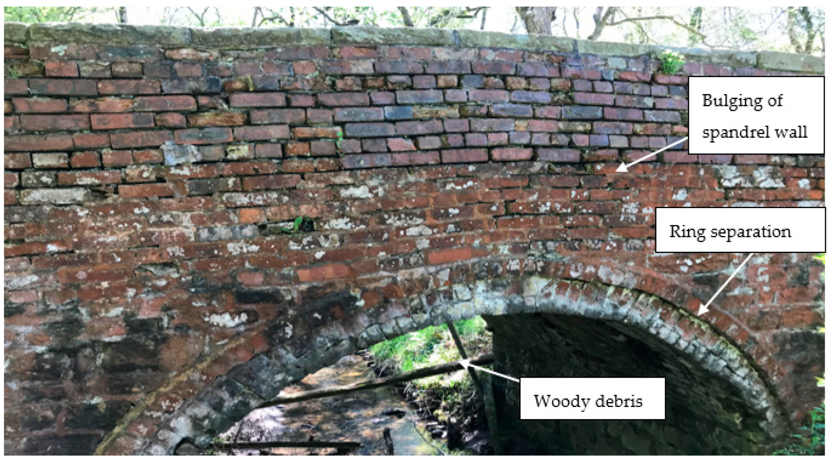
:1. Introduction
2. Experimental Investigation
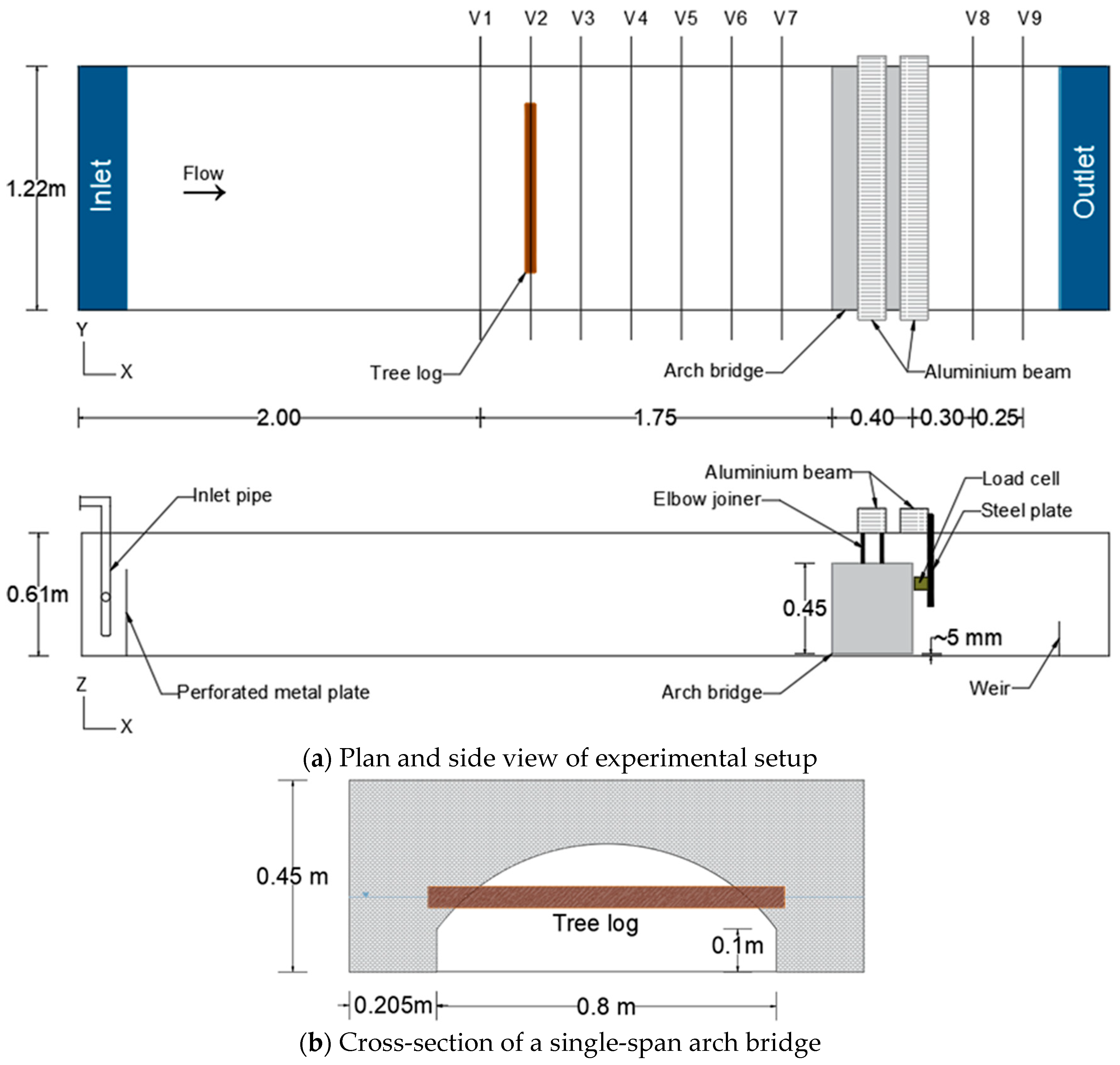
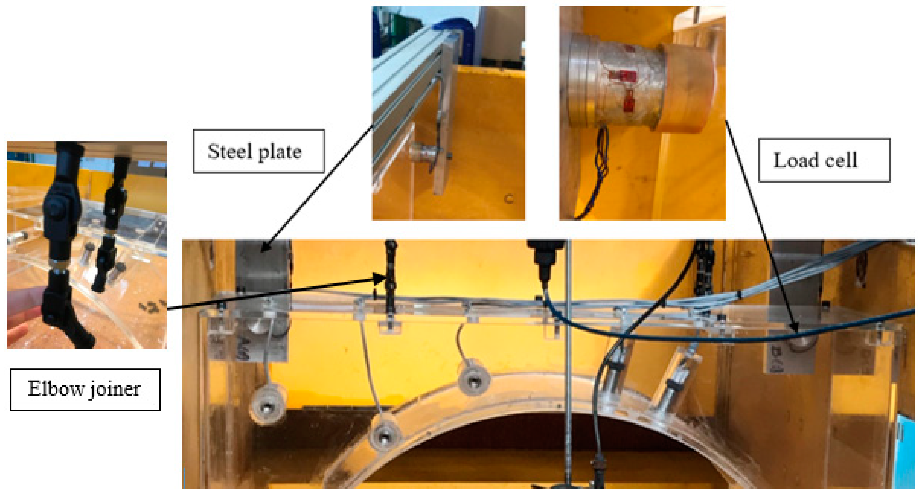
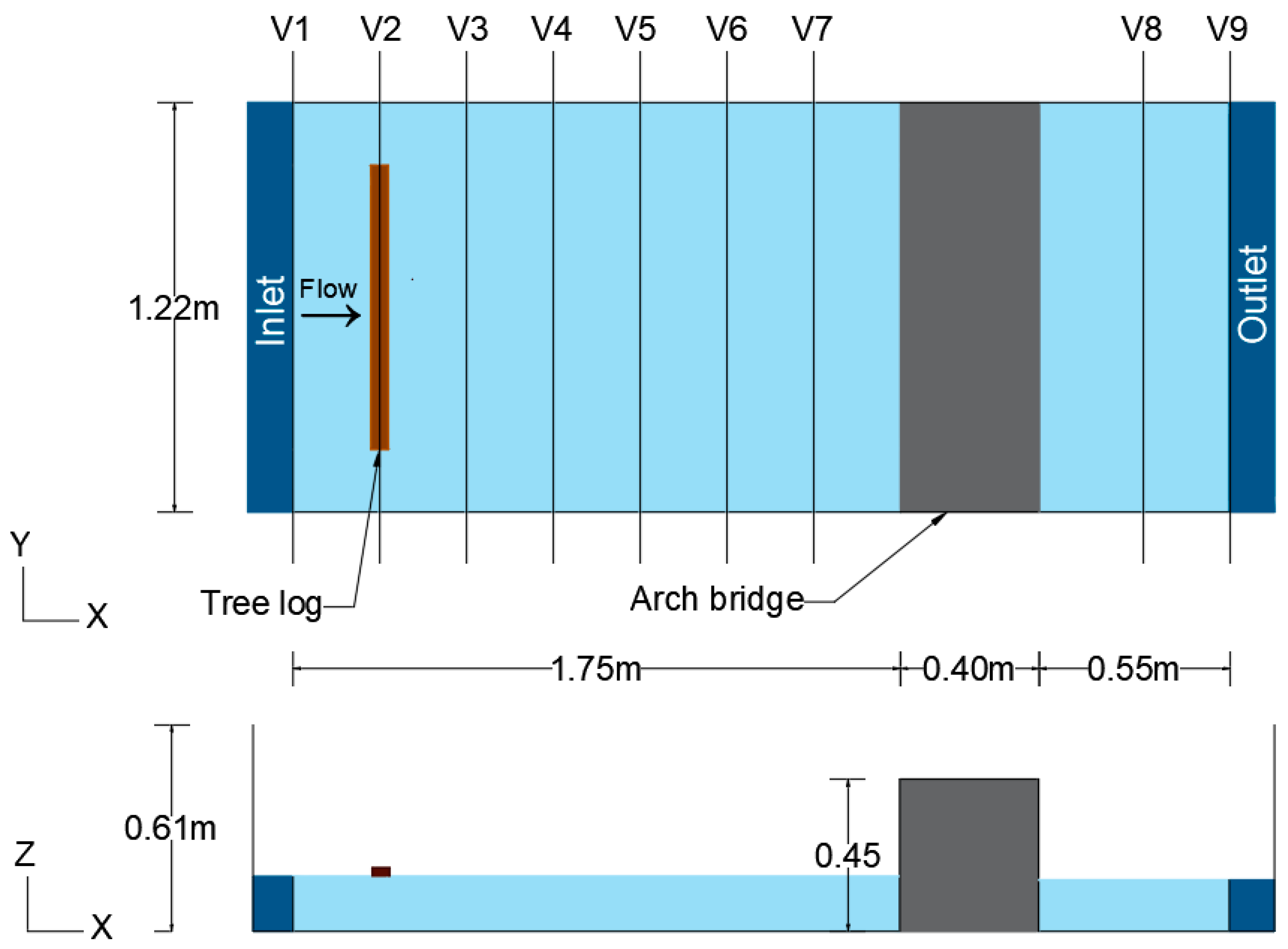
2.1. Experimental Setup
2.2. Test Cases and Data Acquisation
2.3. Results
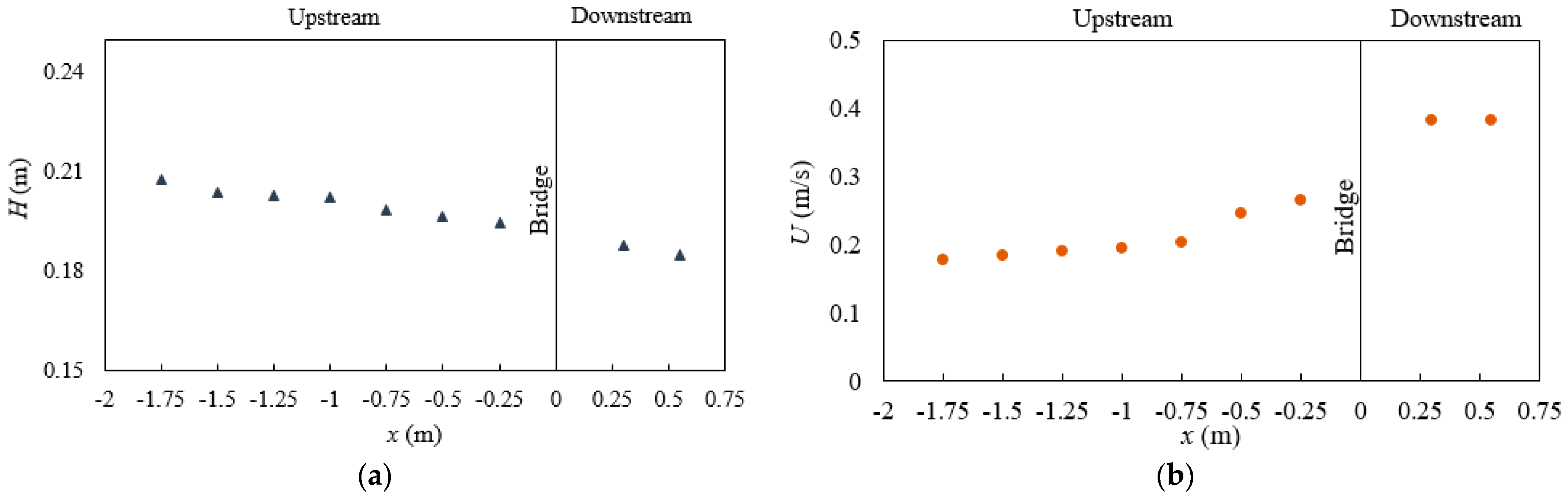
2.3.1. Flow Depths and Depth-Averaged Velocity Profiles
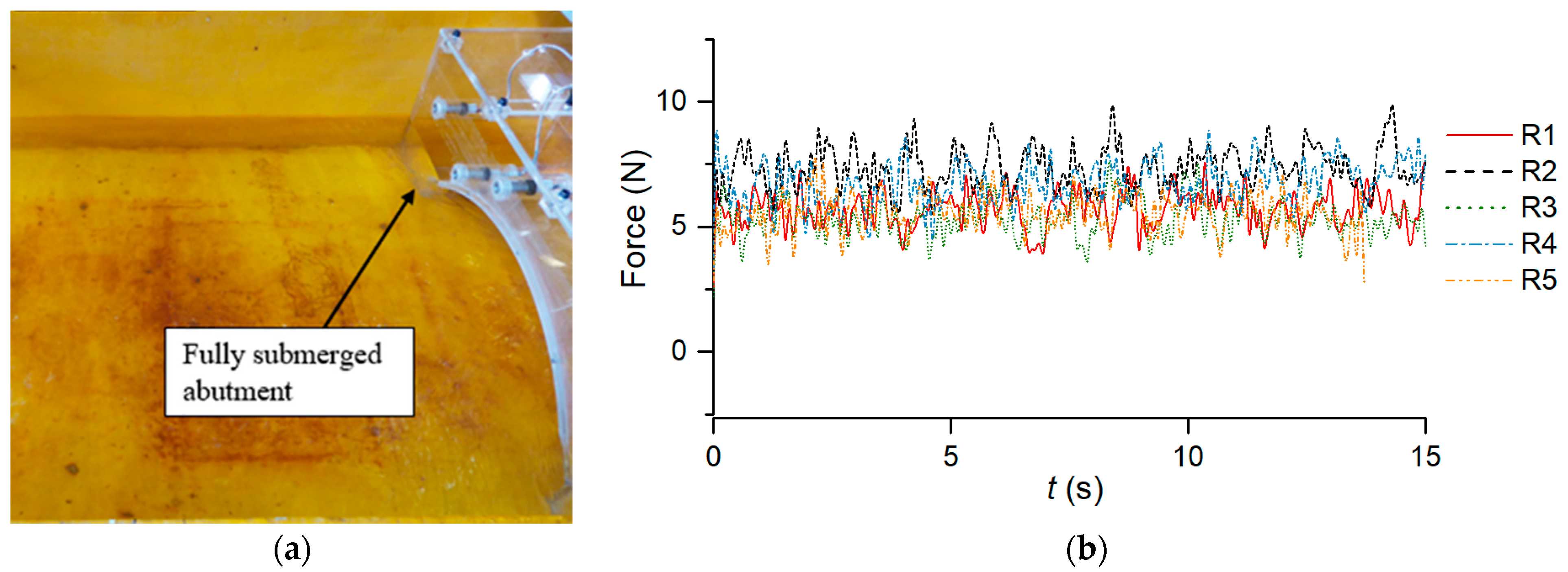
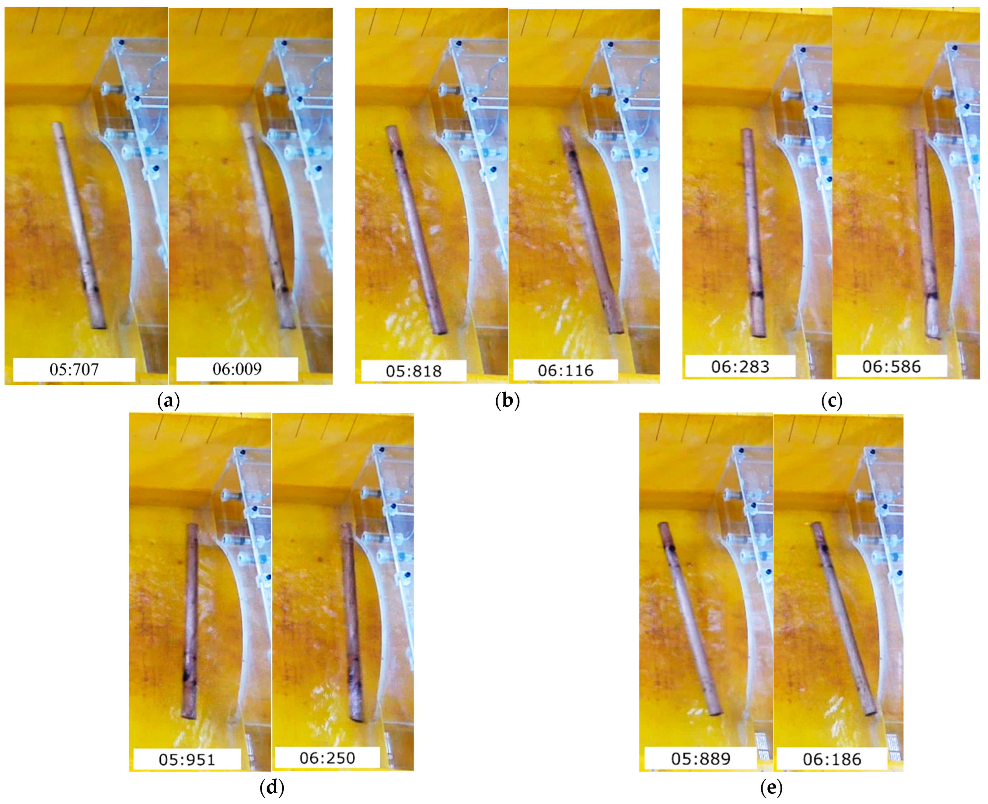
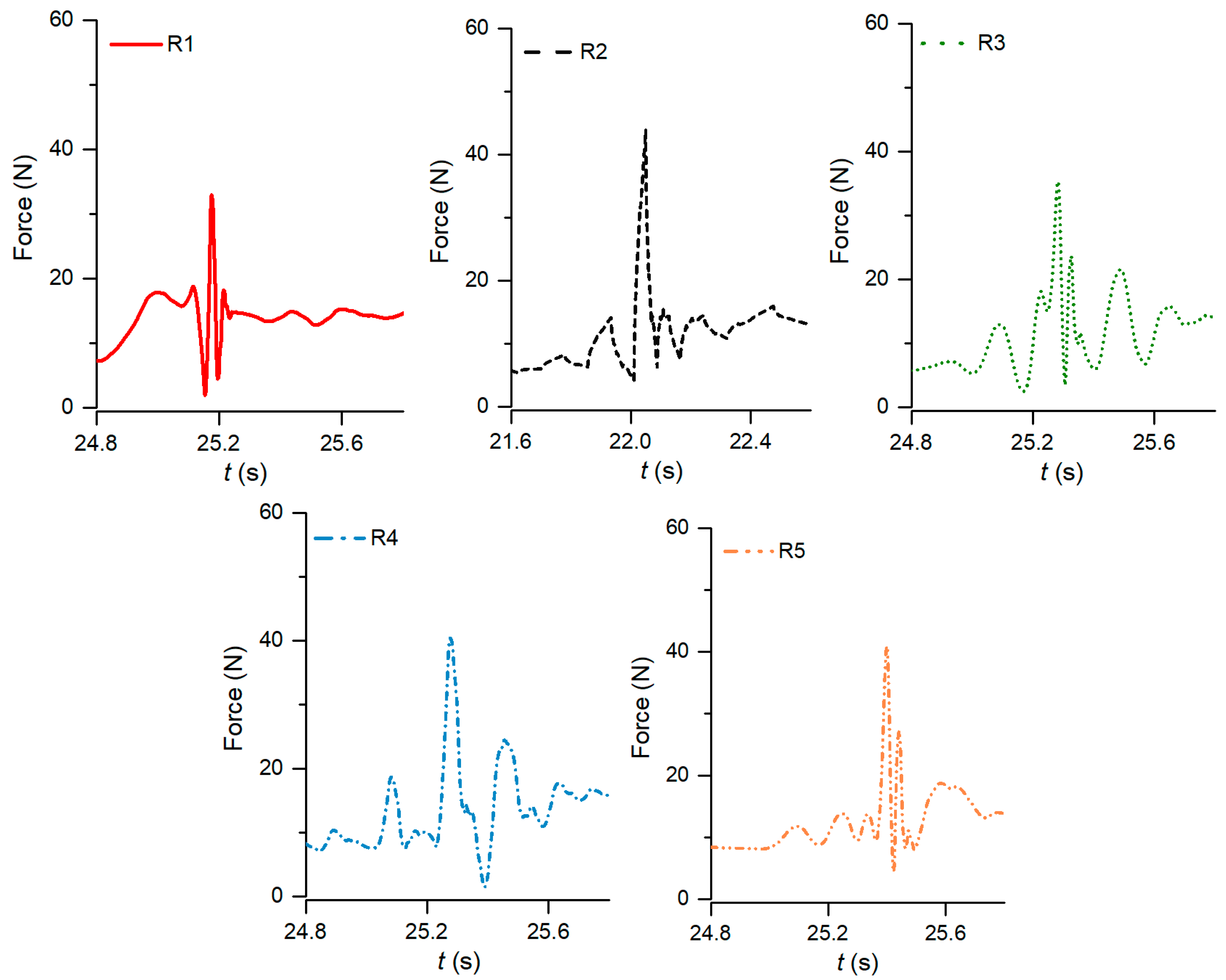
2.3.2. Hydrodynamic and Debris Impact Loads
3. Numerical Investigation: Smoothed Particle Hydrodynamics (SPH)
3.1. Numerical Setup
3.2. Validation of the SPH Model
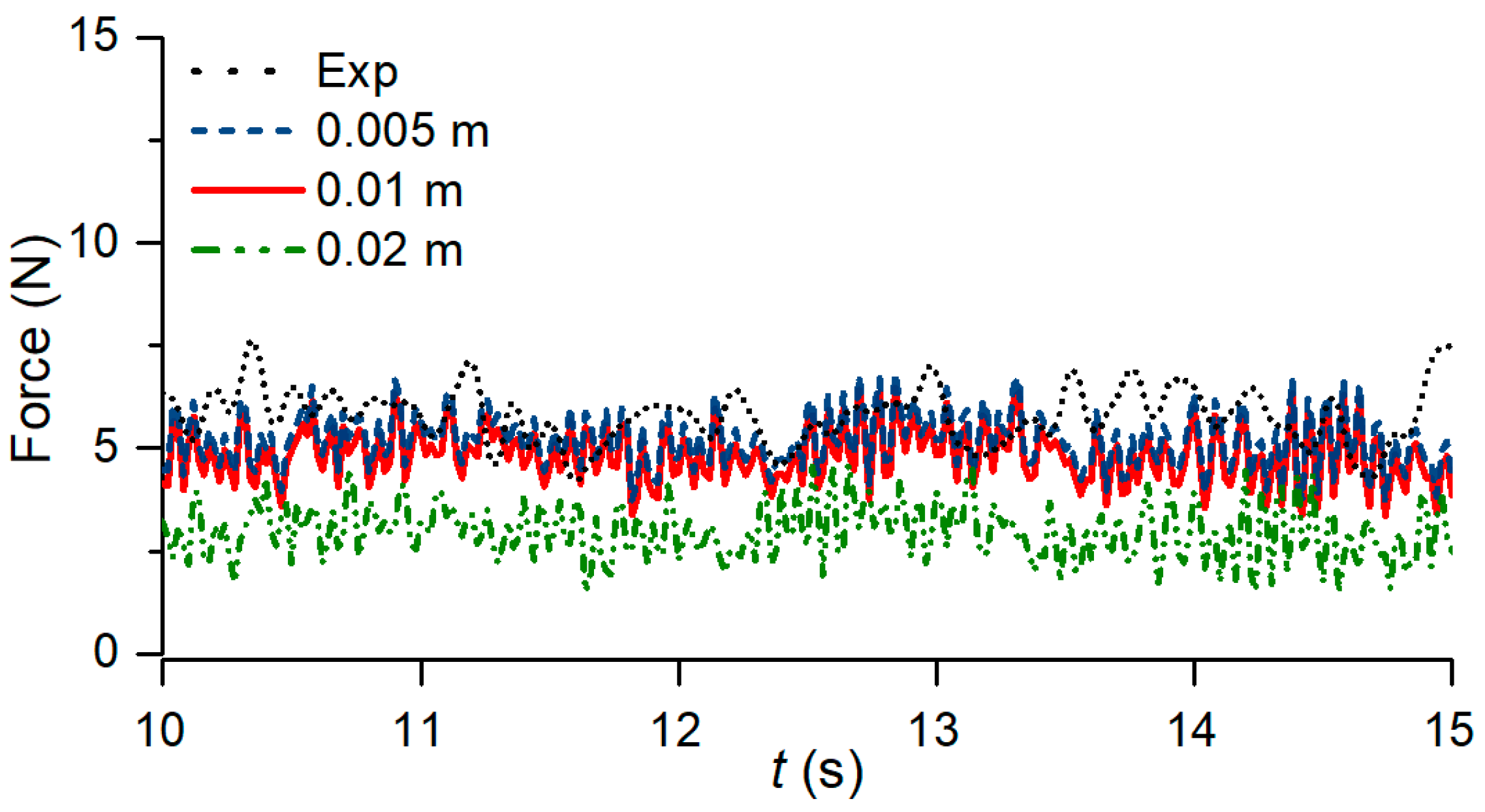
3.2.1. Case 1: Hydrodynamic Load Only
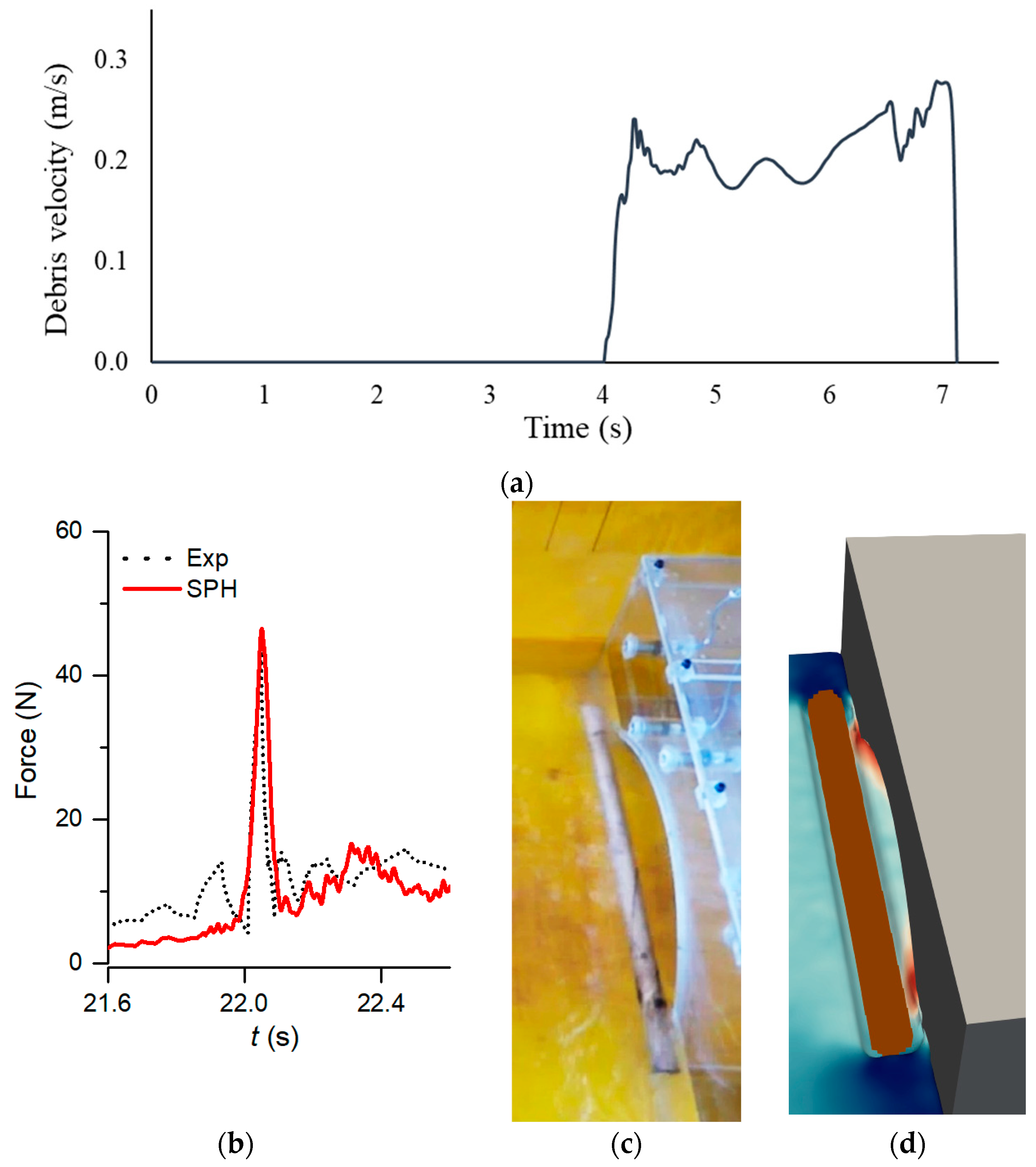
3.2.2. Case 2: Hydrodynamic and Debris Impact Loads
3.3. Further Investigation: Pressure–Time Histories
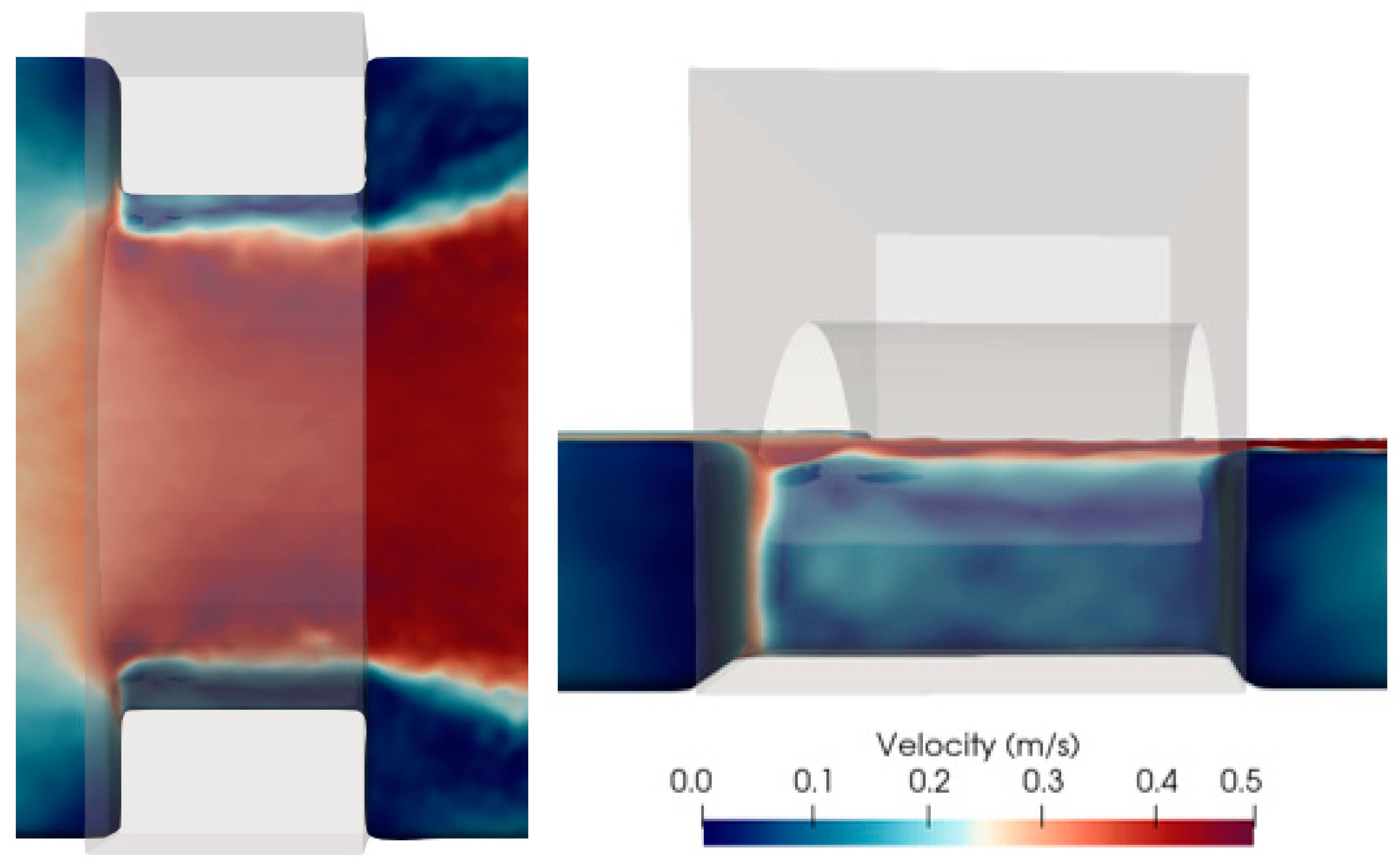
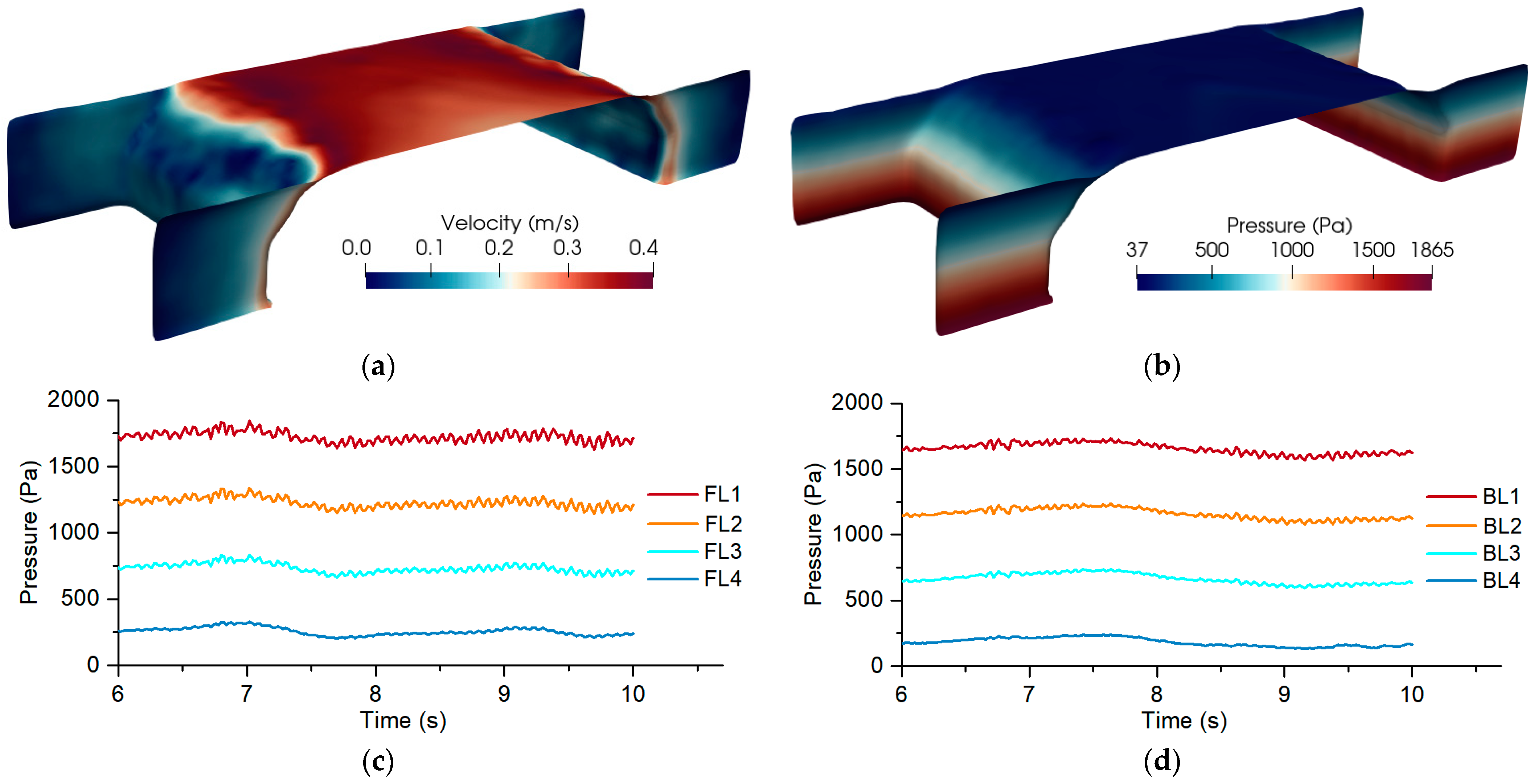
3.3.1. Case 1: Hydrodynamic Load Only
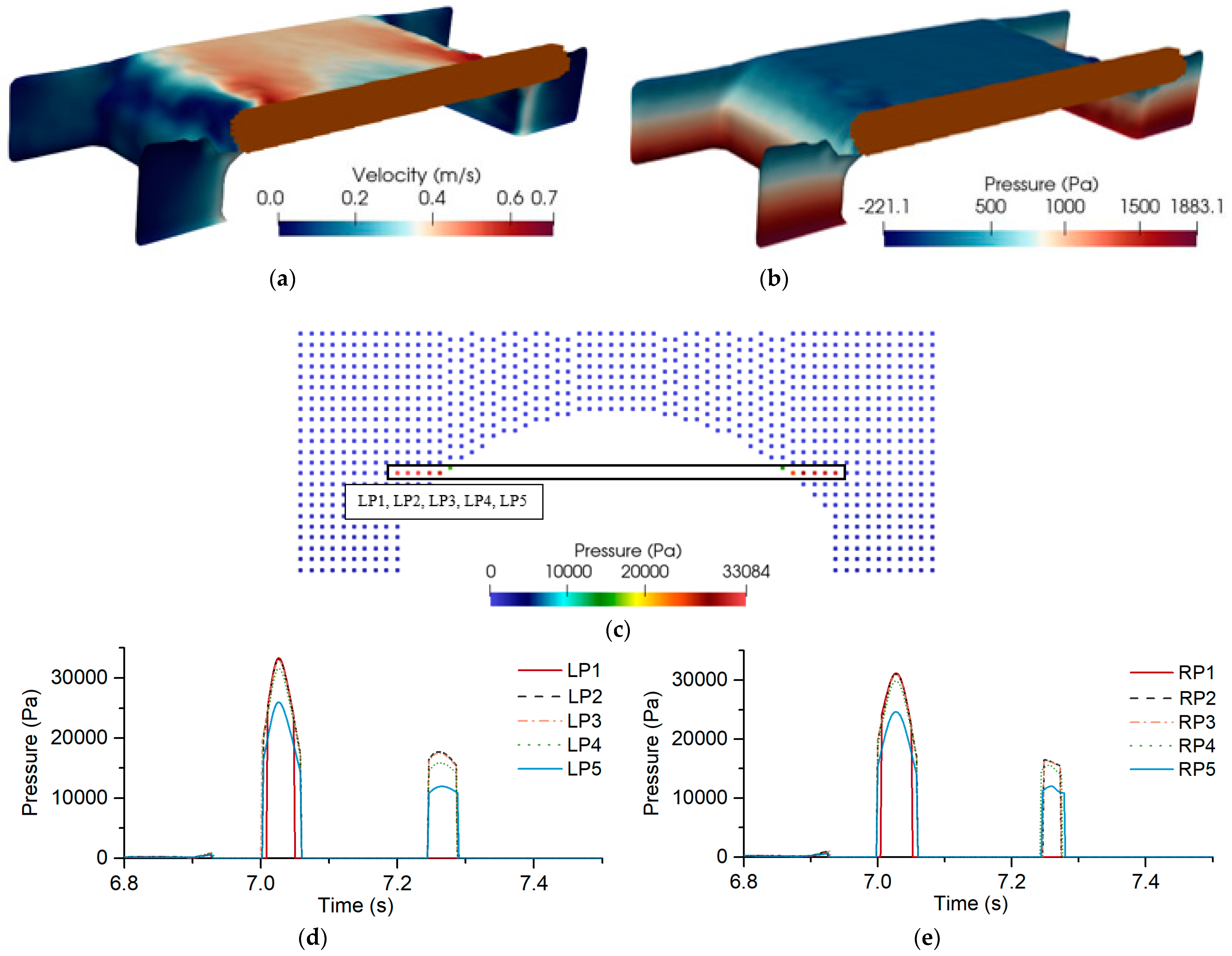
3.3.2. Case 2: Hydrodynamic and Debris Impact Loads
4. Conclusions and Discussions
Author Contributions
Funding
Institutional Review Board Statement
Informed Consent Statement
Data Availability Statement
Acknowledgments
Conflicts of Interest
References
- Hamill, L. Bridge Hydraulics; E & FN Spon: London, UK, 1999. [Google Scholar]
- Proske, D. Bridge Collapse Frequencies versus Failure Probabilities; Springer: Berlin/Heidelberg, Germany, 2018; ISBN 3319738321. [Google Scholar]
- Štulc, J. The 2002 Floods in the Czech Republic and their Impact on Built Heritage. Herit. Risk 2015, 133–138. [Google Scholar] [CrossRef]
- Xia, J.; Teo, F.Y.; Falconer, R.A.; Chen, Q.; Deng, S. Hydrodynamic experiments on the impacts of vehicle blockages at bridges. J. Flood Risk Manag. 2018, 11, S395–S402. [Google Scholar] [CrossRef]
- Padgett, J.; Desroches, R.; Nielson, B.; Yashinsky, M.; Kwon, O.-S.; Burdette, N.; Tavera, E. Bridge Damage and Repair Costs from Hurricane Katrina. J. Bridg. Eng. 2008, 13, 6–14. [Google Scholar] [CrossRef] [Green Version]
- Majtan, E.; Cunningham, L.S.; Rogers, B.D. Flood-induced Hydrodynamic and Debris Impact Forces on Single-span Masonry Arch Bridge. J. Hydraul. Eng. 2021, 147, 04021043. [Google Scholar] [CrossRef]
- Orbán, Z. UIC Project on assessment, inspection and maintenance of masonry arch railway bridges. In Proceedings of the 5th International Conference on Arch Bridges, Madeira, Portugal, 12–14 September 2007; Volume 7, pp. 3–12. [Google Scholar]
- Proske, D.; van Gelder, P. Safety of Historical Stone Arch Bridges; Springer: Berlin/Heidelberg, Germany, 2009; ISBN 9783540776161. [Google Scholar]
- Proske, D.; Hubl, J. Historical arch bridges under horizontal loads. In Proceedings of the 5th International Conference on Arch Bridges, Madeira, Portugal, 12–14 September 2007; Volume 100. [Google Scholar]
- BD 97/12; The Assessment of Scour and Other Hydraulic Actions at Highway Structures. National Highways: London, UK, 2012; Volume 3.
- Takano, H.; Pooley, M. New UK guidance on hydraulic actions on highway structures and bridges. Proc. Inst. Civ. Eng. Bridg. Eng. 2021, 174, 231–238. [Google Scholar] [CrossRef]
- Diehl, T.H. Potential Drift Accumulation at Bridges; US Department of Transportation, Federal Highway Administration, Research and Development, Turner-Fairbank Highway Research Center: McLean, VA, USA, 1997.
- Parola, A.C.; Apelt, C.J.; Jempson, M.A. NCHRP Report 445: Debris Forces on Highway Bridges; Transportation Research Board (TRB), National Research Council: Washington, DC, USA, 2000. [Google Scholar]
- CD 356; Design of Highway Structures for Hydraulic Action. National Highways: London, UK, 2020.
- AS5100.2:2017; Bridge Design Loads. Australian Standard: Sydney, NSW, Australia, 2017; Volume 4.
- May, R.W.P.; Ackers, J.C.; Kirby, A.M. Manual on Scour at Bridges and Other Hydraulic Structures (C742); Ciria: London, UK, 2017; ISBN 0860175510. [Google Scholar]
- FHWA. Hydrodynamic Forces on Inundated Bridge Decks; FHWA: Washington, DC, USA, 2009.
- Robertson, I.N.; Riggs, H.R.; Yim, S.C.; Young, Y.L. Lessons from Hurricane Katrina Storm Surge on Bridges and Buildings. J. Waterw. Port Coast. Ocean. Eng. 2007, 133, 463–483. [Google Scholar] [CrossRef]
- Ettema, R.; Arndt, R.; Roberts, P.; Wahl, T. Hydraulic Modeling: Concepts and Practice; American Society of Civil Engineers: Reston, VA, USA, 2000; ISBN 0784404151. [Google Scholar]
- Panici, D.; Kripakaran, P. Assessing and mitigating risks to bridges from large wood using satellite imagery. Proc. Inst. Civ. Eng. Bridg. Eng. 2021, 1–11. [Google Scholar] [CrossRef]
- Hasanpour, A.; Istrati, D.; Buckle, I. Coupled sph–fem modeling of tsunami-borne large debris flow and impact on coastal structures. J. Mar. Sci. Eng. 2021, 9, 1068. [Google Scholar] [CrossRef]
- Haehnel, R.B.; Daly, S.F. Maximum Impact Force of Woody Debris on Floodplain Structures. J. Hydraul. Eng. 2004, 130, 112–120. [Google Scholar] [CrossRef]
- Stolle, J.; Nistor, I.; Goseberg, N.; Petriu, E. Multiple Debris Impact Loads in Extreme Hydrodynamic Conditions. J. Waterw. Port Coast. Ocean. Eng. 2020, 146, 04019038. [Google Scholar] [CrossRef]
- Andersson, B.; Andersson, R.; Håkansson, L.; Mortensen, M.; Sudiyo, R.; Van Wachem, B. Computational Fluid Dynamics for Engineers; Cambridge University Press: Cambridge, UK, 2011; Volume 9781107018, ISBN 9781139093590. [Google Scholar]
- Istrati, D.; Buckle, I.G. Tsunami Loads on Straight and Skewed Bridges—Part 2: Numerical Investigation and Design Recommendations; Oregon Department of Transportation: Salem, OR, USA, 2021.
- Zhu, M.; Elkhetali, I.; Scott, M.H. Validation of OpenSees for Tsunami Loading on Bridge Superstructures. J. Bridg. Eng. 2018, 23, 04018015. [Google Scholar] [CrossRef]
- Xiang, T.; Istrati, D. Assessment of extreme wave impact on coastal decks with different geometries via the arbitrary lagrangian-eulerian method. J. Mar. Sci. Eng. 2021, 9, 1342. [Google Scholar] [CrossRef]
- Shadloo, M.S.; Oger, G.; Le Touzé, D. Smoothed particle hydrodynamics method for fluid flows, towards industrial applications: Motivations, current state, and challenges. Comput. Fluids 2016, 136, 11–34. [Google Scholar] [CrossRef]
- Erduran, K.S.; Seckin, G.; Kocaman, S.; Atabay, S. 3D numerical modelling of flow around skewed bridge crossing. Eng. Appl. Comput. Fluid Mech. 2012, 6, 475–489. [Google Scholar] [CrossRef] [Green Version]
- Hartana; Murakami, K.; Yamaguchi, Y.; Maki, D. 2-Phase Flow Analysis of Tsunami Forces Acting on Bridge Structures. J. Jpn. Soc. Civ. Eng. Ser. B3 Ocean. Eng. 2013, 69, I_347–I_352. [Google Scholar] [CrossRef] [Green Version]
- Chu, C.-R.; Chung, C.-H.; Wu, T.-R.; Wang, C.-Y. Numerical Analysis of Free Surface Flow over a Submerged Rectangular Bridge Deck. J. Hydraul. Eng. 2016, 142, 04016060. [Google Scholar] [CrossRef]
- Ebrahimi, M.; Kahraman, R.; Kripakaran, P.; Djordjević, S.; Tabor, G.; Prodanović, D.M.; Arthur, S.; Riella, M. Scour and Hydrodynamic Effects of Debris Blockage at Masonry Bridges: Insights from Experimental and Numerical Modelling. In Proceedings of the 37th International Association for Hydro-Environment Engineering and Research (IAHR) Congress, Kuala Lumpur, Malaysia, 14–18 August 2017. [Google Scholar]
- Nasim, M.; Setunge, S.; Zhou, S.; Mohseni, H. An investigation of water-flow pressure distribution on bridge piers under flood loading. Struct. Infrastruct. Eng. 2019, 15, 219–229. [Google Scholar] [CrossRef]
- Oudenbroek, K.; Naderi, N.; Bricker, J.D.; Yang, Y.; van der Veen, C.; Uijttewaal, W.; Moriguchi, S.; Jonkman, S.N. Hydrodynamic and debris-damming failure of bridge decks and piers in steady flow. Geosciences 2018, 8, 409. [Google Scholar] [CrossRef] [Green Version]
- Kahraman, R.; Riella, M.; Tabor, G.R.; Ebrahimi, M.; Djordjević, S.; Kripakaran, P. Prediction of flow around a sharp-nosed bridge pier: Influence of the Froude number and free-surface variation on the flow field. J. Hydraul. Res. 2019, 1686, 582–583. [Google Scholar] [CrossRef] [Green Version]
- Benzi, R.; Succi, S.; Vergassola, M. The lattice Boltzmann equation: Theory and applications. Phys. Rep. 1992, 222, 145–197. [Google Scholar] [CrossRef]
- Rothman, D.; Zaleski, S. Lattice-Gas Cellular Automata: Simple Models of Complex Hydrodynamics; Cambridge University Press: Cambridge, UK, 2004. [Google Scholar]
- Shimizu, Y.; Gotoh, H.; Khayyer, A. An MPS-based particle method for simulation of multiphase flows characterized by high density ratios by incorporation of space potential particle concept. Comput. Math. Appl. 2018, 76, 1108–1129. [Google Scholar] [CrossRef]
- Khayyer, A.; Gotoh, H.; Falahaty, H.; Shimizu, Y. An enhanced ISPH–SPH coupled method for simulation of incompressible fluid–elastic structure interactions. Comput. Phys. Commun. 2018, 232, 139–164. [Google Scholar] [CrossRef]
- Colagrossi, A.; Landrini, M. Numerical simulation of interfacial flows by smoothed particle hydrodynamics. J. Comput. Phys. 2003, 191, 448–475. [Google Scholar] [CrossRef]
- Oger, G.; Doring, M.; Alessandrini, B.; Ferrant, P. An improved SPH method: Towards higher order convergence. J. Comput. Phys. 2007, 225, 1472–1492. [Google Scholar] [CrossRef]
- Liu, M.B.; Liu, G.R. Smoothed particle hydrodynamics (SPH): An overview and recent developments. Arch. Comput. Methods Eng. 2010, 17, 25–76. [Google Scholar] [CrossRef] [Green Version]
- Marrone, S.; Colagrossi, A.; Antuono, M.; Colicchio, G.; Graziani, G. An accurate SPH modeling of viscous flows around bodies at low and moderate Reynolds numbers. J. Comput. Phys. 2013, 245, 456–475. [Google Scholar] [CrossRef]
- Monaghan, J.J.; Rafiee, A. A simple SPH algorithm for multi-fluid flow with high densityratios. Int. J. Numer. Methods Fluids 2013, 71, 537–561. [Google Scholar] [CrossRef]
- Zhao, T. Investigation of Landslide-Induced Debris Flows by the DEM and CFD. Ph.D. Thesis, University of Oxford, Oxford, UK, 2014; 251p. [Google Scholar]
- Canelas, R.B.; Crespo, A.J.C.; Domínguez, J.M.; Ferreira, R.M.L.; Gómez-Gesteira, M. SPH-DCDEM model for arbitrary geometries in free surface solid-fluid flows. Comput. Phys. Commun. 2016, 202, 131–140. [Google Scholar] [CrossRef]
- Capasso, S.; Tagliafierro, B.; Martínez-Estévez, I.; Domínguez, J.M.; Crespo, A.J.C.; Viccione, G. A DEM approach for simulating flexible beam elements with the Project Chrono core module in DualSPHysics. Comput. Part. Mech. 2022, 1–17. [Google Scholar] [CrossRef]
- Khayyer, A.; Tsuruta, N.; Shimizu, Y.; Gotoh, H. Multi-resolution MPS for incompressible fluid-elastic structure interactions in ocean engineering. Appl. Ocean Res. 2019, 82, 397–414. [Google Scholar] [CrossRef]
- Istrati, D.; Buckle, I.G. Effect of Fluid-Structure Interaction on Connection Forces in Bridges due to Tsunami Loads. In Proceedings of the 30th US-Japan Bridge Engineering Workshop, Washington, DC, USA, 21 October 2014; pp. 21–23. [Google Scholar]
- Al-Faesly, T.Q.; Nistor, I.; Palermo, D.; Cornett, A. Experimental study of structures subjected to hydrodynamic and debris impact forces. In Proceedings of the Annual Conference of the Canadian Society for Civil Engineering, Montreal, QC, Canada, 29 May–1 June 2013; Volume 1, pp. 118–127. [Google Scholar]
- Ducrocq, T.; Cassan, L.; Chorda, J.; Roux, H. Flow and drag force around a free surface piercing cylinder for environmental applications. Environ. Fluid Mech. 2017, 17, 629–645. [Google Scholar] [CrossRef] [Green Version]
- Boothby, T.E.; Roberts, B.J. Transverse behaviour of masonry arch bridges. Struct. Eng. 2001, 79, 21–26. [Google Scholar]
- Comiti, F.; Andreoli, A.; Lenzi, M.A.; Mao, L. Spatial density and characteristics of woody debris in five mountain rivers of the Dolomites (Italian Alps). Geomorphology 2006, 78, 44–63. [Google Scholar] [CrossRef]
- Magilligan, F.J.; Nislow, K.H.; Fisher, G.B.; Wright, J.; Mackey, G.; Laser, M. The geomorphic function and characteristics of large woody debris in low gradient rivers, coastal Maine, USA. Geomorphology 2008, 97, 467–482. [Google Scholar] [CrossRef]
- Ebrahimi, M.; Kripakaran, P.; Prodanović, D.M.; Kahraman, R.; Riella, M.; Tabor, G.; Arthur, S.; Djordjević, S. Experimental Study on Scour at a Sharp-Nose Bridge Pier with Debris Blockage. J. Hydraul. Eng. 2018, 144, 04018071. [Google Scholar] [CrossRef] [Green Version]
- Heller, V. Scale effects in physical hydraulic engineering models. J. Hydraul. Res. 2011, 49, 293–306. [Google Scholar] [CrossRef]
- Mathews, R.; Hardman, M. Lessons learnt from the December 2015 flood event in Cumbria, UK. Proc. Inst. Civ. Eng. Forensic Eng. 2017, 170, 165–178. [Google Scholar] [CrossRef]
- Istrati, D.; Hasanpour, A.; Buckle, I.G. Numerical Investigation of Tsunami-Borne Debris Damming Loads on a Coastal Bridge. In Proceedings of the 17 World Conference on Earthquake Engineering, Sendai, Japan, 27 September 2020; pp. 1–12. [Google Scholar]
- Jeffcoate, P. Experimental and Computational Modelling of 3D Flow and Bed Shear Stresses Downstream from a Multiple Duct Tidal Barrage; The University of Manchester: Manchester, UK, 2013; pp. 1–345. [Google Scholar]
- Nortek, A.S. The Comprehensive Manual for Velocimeters; Nortek AS: Rud, Norway, 2018. [Google Scholar]
- Ficker, T.; Martišek, D. 3D Image Reconstructions and the Nyquist–Shannon Theorem. 3D Res. 2015, 6, 23. [Google Scholar] [CrossRef]
- Robertson, I.N.; Riggs, H.R.; Mohamed, A. Experimental results of tsunami bore forces on structures. Proc. Int. Conf. Offshore Mech. Arct. Eng.-OMAE 2008, 1, 509–517. [Google Scholar] [CrossRef] [Green Version]
- Istrati, D. Large-Scale Experiments of Tsunami Inundation of Bridges including Copyright by Denis Istrati 2017 All Rights Reserved. Ph.D. Thesis, University of Nevada, Reno, Nevada, 2017. [Google Scholar]
- English, A.; Domínguez, J.M.; Vacondio, R.; Crespo, A.J.C.; Stansby, P.K.; Lind, S.J.; Chiapponi, L.; Gómez-Gesteira, M. Modified dynamic boundary conditions (mDBC) for general-purpose smoothed particle hydrodynamics (SPH): Application to tank sloshing, dam break and fish pass problems. Comput. Part. Mech. 2021, 1–15. [Google Scholar] [CrossRef]
- Pringgana, G.; Cunningham, L.S.; Rogers, B.D. Modelling of tsunami-induced bore and structure interaction. Proc. Inst. Civ. Eng. Eng. Comput. Mech. 2016, 169, 109–125. [Google Scholar] [CrossRef] [Green Version]
- Baines, A.; Watson, P.; Cunningham, L.S.; Rogers, B.D.; Murphy, J.; Lizondo, S. Modelling shore-side pressure distributions from violent wave breaking at a seawall. Proc. Inst. Civ. Eng. Eng. Comput. Mech. 2019, 172, 118–123. [Google Scholar] [CrossRef]


| Case | Flow Depth at V1 (m) | Flow Rate (m3/s) | Fr | Re | Debris |
|---|---|---|---|---|---|
| 1 | 0.208 | 0.0436 | 0.120 | 35,724 | - |
| 2 | 0.208 | 0.0436 | 0.120 | 35,724 | Tree log |
| Reading No. | ForceRMS (N) |
|---|---|
| R1 | 5.74 |
| R2 | 7.39 |
| R3 | 5.40 |
| R4 | 6.78 |
| R5 | 5.62 |
| Mean | 6.19 |
| SD | 0.77 |
| COV, % | 12.40 |
| Reading No. | ForcePeak (N) | uDebris (m/s) |
|---|---|---|
| R1 | 32.94 | 0.331 |
| R2 | 43.92 | 0.336 |
| R3 | 35.25 | 0.330 |
| R4 | 40.40 | 0.334 |
| R5 | 40.84 | 0.337 |
| Mean | 38.67 | 0.334 |
| SD | 4.00 | 0.003 |
| COV, % | 10.33 | 0.818 |
| Flow Depth at V1 (m) | Particle Size, dp (m) | ForceRMS (N) | Error (%) | Total Particle | Total Run Time |
|---|---|---|---|---|---|
| 0.208 | 0.005 | 5.25 | 15.19 | 7,931,232 | 21 h 13 min |
| 0.208 | 0.01 | 5.10 | 17.61 | 1,873,208 | 2 h 49 min |
| 0.208 | 0.02 | 3.82 | 38.29 | 348,336 | 23 min |
| Front (F) | Back (B) | ||
|---|---|---|---|
| Name | Measurement Point (x,y,z) | Name | Measurement Point (x,y,z) |
| FL1 | 1.75, 0.2, 0.03 | BL1 | 2.15, 0.2, 0.03 |
| FL2 | 1.75, 0.2, 0.08 | BL2 | 2.15, 0.2, 0.08 |
| FL3 | 1.75, 0.2, 0.13 | BL3 | 2.15, 0.2, 0.13 |
| FL4 | 1.75, 0.2, 0.18 | BL4 | 2.15, 0.2, 0.18 |
Publisher’s Note: MDPI stays neutral with regard to jurisdictional claims in published maps and institutional affiliations. |
© 2022 by the authors. Licensee MDPI, Basel, Switzerland. This article is an open access article distributed under the terms and conditions of the Creative Commons Attribution (CC BY) license (https://creativecommons.org/licenses/by/4.0/).
Share and Cite
Majtan, E.; Cunningham, L.S.; Rogers, B.D. Experimental and Numerical Investigation of Floating Large Woody Debris Impact on a Masonry Arch Bridge. J. Mar. Sci. Eng. 2022, 10, 911. https://0-doi-org.brum.beds.ac.uk/10.3390/jmse10070911
Majtan E, Cunningham LS, Rogers BD. Experimental and Numerical Investigation of Floating Large Woody Debris Impact on a Masonry Arch Bridge. Journal of Marine Science and Engineering. 2022; 10(7):911. https://0-doi-org.brum.beds.ac.uk/10.3390/jmse10070911
Chicago/Turabian StyleMajtan, Eda, Lee S. Cunningham, and Benedict D. Rogers. 2022. "Experimental and Numerical Investigation of Floating Large Woody Debris Impact on a Masonry Arch Bridge" Journal of Marine Science and Engineering 10, no. 7: 911. https://0-doi-org.brum.beds.ac.uk/10.3390/jmse10070911