Simulating Destructive and Constructive Morphodynamic Processes in Steep Beaches


1
CIMA–Centre for Marine and Environmental Research, FCT, Campus de Gambelas, Universidade do Algarve, 8005-139 Faro, Portugal
2
Water Science and Engineering Department, IHE Delft institute for Water Education, Westvest 7, 2611 AX Delft, The Netherlands
*
Author to whom correspondence should be addressed.
J. Mar. Sci. Eng. 2021, 9(1), 86; https://0-doi-org.brum.beds.ac.uk/10.3390/jmse9010086
Submission received: 14 December 2020
/
Revised: 7 January 2021
/
Accepted: 12 January 2021
/
Published: 15 January 2021
(This article belongs to the Special Issue Monitoring and Modelling of Coastal Environment)
Abstract
:Short-term beach morphodynamics are typically modelled solely through storm-induced erosion, disregarding post-storm recovery. Yet, the full cycle of beach profile response is critical to simulating and understanding morphodynamics over longer temporal scales. The XBeach model is calibrated using topographic profiles from a reflective beach (Faro Beach, in S. Portugal) during and after the incidence of a fierce storm (Emma) that impacted the area in early 2018. Recovery in all three profiles showed rapid steepening of the beachface and significant recovery of eroded volumes (68–92%) within 45 days after the storm, while berm heights reached 4.5–5 m. Two calibration parameters were used (facua and bermslope), considering two sets of values, one for erosive (Hm0 ≥ 3 m) and one for accretive (Hm0 < 3 m) conditions. A correction of the runup height underestimation by the model in surfbeat mode was necessary to reproduce the measured berm elevation and morphology during recovery. Simulated profiles effectively capture storm erosion, but also berm growth and gradual recovery of the profiles, showing good skill in all three profiles and recovery phases. These experiments will be the basis to formulate event-scale simulations using schematized wave forcing that will allow to calibrate the model for longer-term changes.
1. Introduction
Cross-shore beach changes occur over a wide range of timescales, from episodic events (storms) to decades, and can involve detrimental impacts to coastal ecosystems, natural and artificial defenses, infrastructure and safety [1]. In fact, long-term coastal change is dictated by the balance between erosion and recovery over significantly shorter timescales [2]. Even though there is increasing consensus that the interacting and coupled processes at shorter timescales are crucial to coastal changes even over climate change timeframes [3], coastal management decisions are still usually based on annual to decadal scales, disregarding short-term beach variability [4].
Therefore, understanding short-term (hours to months) coastal change is essential for assessing the longer-term (years to decades) beach response. Most short-term studies and modelling efforts focus on storm-induced beach erosion from a single storm or a sequence of storms and only on flooding and erosion hazards [5]. Post-storm beach recovery mechanisms play a critical role for future coastal evolution modelling [6], not only for the marine-dominated zones, but for the entire beach-dune system. The transfer of sediment from the nearshore to the beach during milder conditions, driven by the combination of cross-shore and long-shore processes, controls the recovery and growth of the subaerial profile, providing space for recolonization and expansion of dune-building vegetation and/or sediment that winds can transfer to the backshore and dune [7].
Despite the importance of the post-storm beach recovery phase, and even though the antecedent beach morphology is a key parameter for assessing storm impacts [8], it is significantly less studied than beach erosion response, while it is often neglected even in storm sequencing studies [9,10]. Especially for steep, dynamic, beaches, where erosion and recovery processes translate to more rapid morphological changes, related studies are even more scarce [11]. At the same time, current state-of-the-art coastal morphodynamic models (e.g., XBeach) are capable of accurately reproducing storm-induced beach erosion, but much work is needed to improve the accuracy of modelled beach response during calm periods, as physical processes governing recovery are poorly understood [9]. Process-based models have mainly been used to study the effect of a single (or a few) storm sequence(s) on beach profiles (short-term influence) [9] (e.g., [12]), or as part of risk reduction measure decision support tools [13]. When accounted for, beach profile post-storm recovery is usually modelled using semi-empirical equilibrium profile models [14,15,16,17]. These are often combined with reduced-complexity shoreline models, such as ShoreFor [18], LX-Shore [19], CoSMoS-COAST [20] and ShorelineS [21], to account for longshore transport gradients. Combinations of process based modelling and equilibrium profile modelling, to determine storm-induced beach erosion and medium to long term evolution associated with climate change impacts, respectively, have also been employed [4].
It follows that there is need to improve the ability of coastal morphodynamic models to predict nearshore morphological erosion and recovery from storms, as a critical first step and basis for building and validating scale aggregated models that operate at higher spatio-temporal scales [22]. The aim of this work is to simulate the short-term morphodynamics of a reflective beach under intense storm erosion and its subsequent recovery, using the XBeach process-based model. The model focuses on cross-shore sand transport processes, that is the dominant component of morphological change over short timescales (hours to months) [23]. The conditions and requirements of these numerical experiments are demanding and well beyond the “comfort zone” of XBeach (storm erosion), especially regarding the challenge of reconstructing steep and high berms under mild wave conditions. Topographic profiles in Faro Beach (Praia de Faro; S. Portugal), measured before, during and after the Emma storm (March 2018), show strong beach erosion, rapid shift of the foreshore morphology to pre-storm conditions and fast recovery, with the bulk of eroded volumes being regained within 45 days. The modelling approach is analyzed in terms of model structure, main calibration parameters and a correction of the predicted runup heights. Results focus on the simulation strengths and weaknesses in reproducing storm and recovery phases and between the profiles and a brief presentation of model sensitivity to the calibration parameter values.
2. Pre- and Post-Storm Beach Response
2.1. Study Area
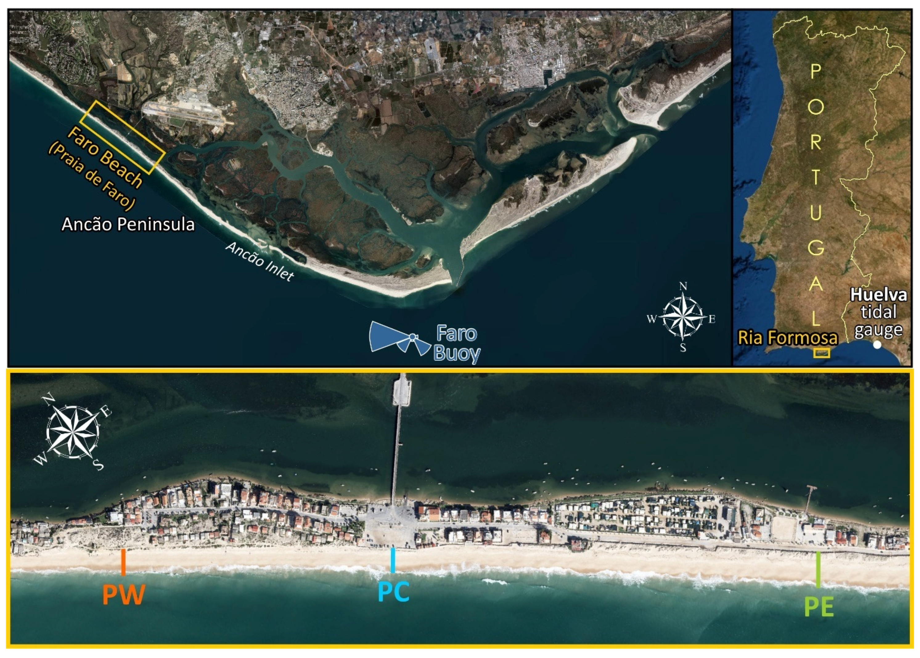
The study concentrates on Faro Beach (Praia de Faro), an inhabited stretch in the central part of Ancão Peninsula, the westmost barrier of Ria Formosa (in S. Portugal; Figure 1), that in early March of 2018 was fiercely impacted by storm Emma, the most recent severe storm in the area, causing strong erosion, overwash in low-lying zones and property damages [13]. Occupation in Faro Beach is recent (since the 1930s) and relatively small (623 buildings, of which 378 lie in the central part). Even though the settlement has experienced repeated storm-induced damages in infrastructure and private buildings, residents seem to underestimate the related risks [24]. In fact, the major coastal hazards in the area have been related to the action of high-energy storms, inducing erosion and overwash [13,24], while the related risks for buildings and infrastructure over this barrier stretch have been assessed as very high [25,26].
Regarding the geomorphological characteristics of the area and the long-term dynamics and driving conditions, Ancão is the narrowest and tallest barrier within Ria Formosa, morphology that is highly related to wave exposure and climate. Both barrier width and dune height decrease from west to east (toward the inlet; ranging from 300 to 50 m and 9.3 to 6.5 m, respectively [27,28,29]), while long-term rates during the last 60 years show dominance of retreat over the zone outside the inlet migration path [29]. In the coastal stretch of Faro Beach (Figure 1), barrier widths are around 100–150 m and long-term erosion rates are around 0.8 m/yr [29]. In terms of beach profile morphology, the nearshore is characterised by a steep beachface, with slopes varying from 6% to 15% and an average value of around 11% [11], with well to very well sorted medium to coarse sand and mean grain sizes of 0.35–0.8 mm [30]. The tidal regime is semi-diurnal, with average neap and spring tidal ranges between 1.3 and 2.8 m, that reach 3.5 m during spring equinoctial tides. The area is mainly exposed to waves from W and SW, corresponding to 71% of wave occurrence [31], leading to a dominant eastward littoral drift along the western flank of Ria Formosa (around 105 m3/yr [32]). Wave storm events are characterised by significant wave heights exceeding 2.5 m to 3 m (after [33] and [31], respectively), while storm variability in terms of wave height and surge is correlated with the North Atlantic Oscillation and the East Atlantic Pattern [34]. Storm-induced coastal retreat in Faro Beach has been estimated at around 15 m [35] to 23–31 m [36], for storms with return periods of 25 and 50 years.
The present work focuses on the storm-induced erosion and subsequent recovery in Faro Beach by the Emma storm (March 2018), with a track similar to some of the most energetic and devastating historical storms in the area [13]. Three profiles (PW, PC and PE; Figure 1) along Faro Beach were monitored during this event (using a GNSS-DGPS system; [32]), with measured profiles before (26 Feb) and right after the storm peak (2 Mar) as well as 6, 35 and 49 days later (8 March and 6 and 20 April).
2.2. Hydrodynamic Data
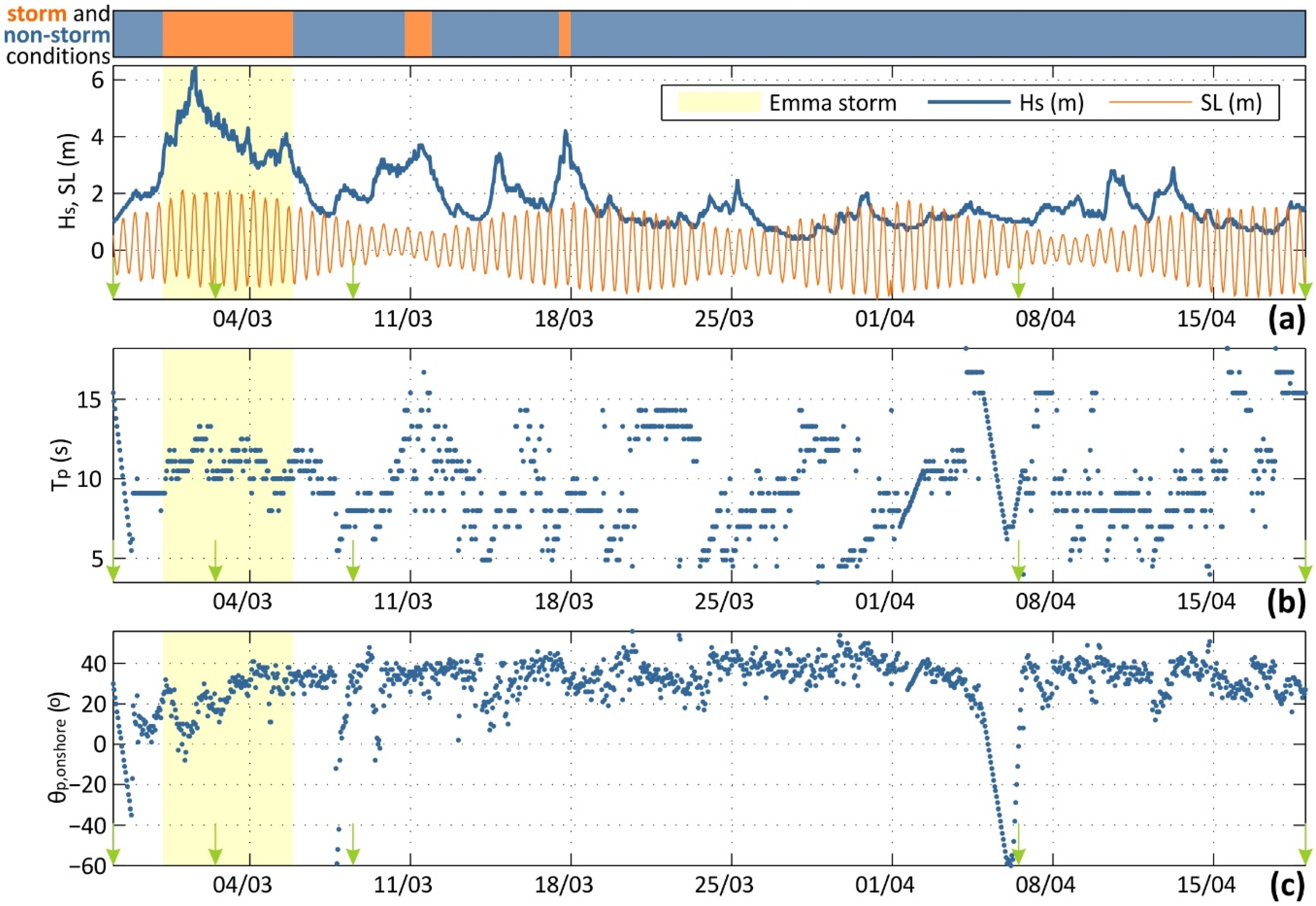
The available hydrodynamic data includes hourly records of offshore waves and sea levels (SL), given in Figure 2 for the duration of the monitoring period (26 February to 20 April 2018). Wave time-series (significant wave height, Hs; peak period, Tp; mean direction associated to peak period, θp) were collected from the Faro buoy, located offshore the study area, at a depth of 93 m (Figure 1). SL were assessed using surge levels obtained by the recordings of the Huelva tidal gauge (Redmar network, Puertos del Estado, station code 3329; Figure 1), corrected for the astronomical tide levels of Faro.
The storm peak of 1st March (Hs = 6.5 m, Tp = 12.5 s and |θp, onshore| < 15°) coincided with high spring tides (range around 3 m) and surge levels of 40 to 60 cm. These conditions caused inundation of the upper beach profile (high surge and runup elevations), resulting to low aeolian sediment transport during the event [32]. Assuming a storm threshold of 3 m for significant wave height [31,37] and a minimum separation window of 6 h between storms [33], the total storm duration was assessed at 5.7 days (28 February 04:00 to 5 March 20:00; shaded area in Figure 2). Two minor storm periods are identified later on (10 March 21:00 to 11 March 20:00 and 17 March 12:00 to 18 March 03:00; see timeline on top of Figure 2). However, the main erosive event of the analysis is the Emma storm and we stress that the terms storm and recovery/post-storm period are used, hereafter, to refer to the Emma event and the rest of the analysis period post-Emma (5 March 21:00 until 20 April), respectively. The corresponding average onshore wave power flux during the storm was 61.3 kW/m/h, value reduced to 8.4 kW/m/h in the rest of the study period (until 20 April). During recovery, longer waves, with peak periods exceeding 13.5 s, were relatively frequent (13.8% occurrence) and associated with wave heights between 0.4 and 3.7 m, short durations (4.4 ± 7.2 h), and an average onshore power flux of 9.5 kW/m/h.
2.3. Morphological Changes
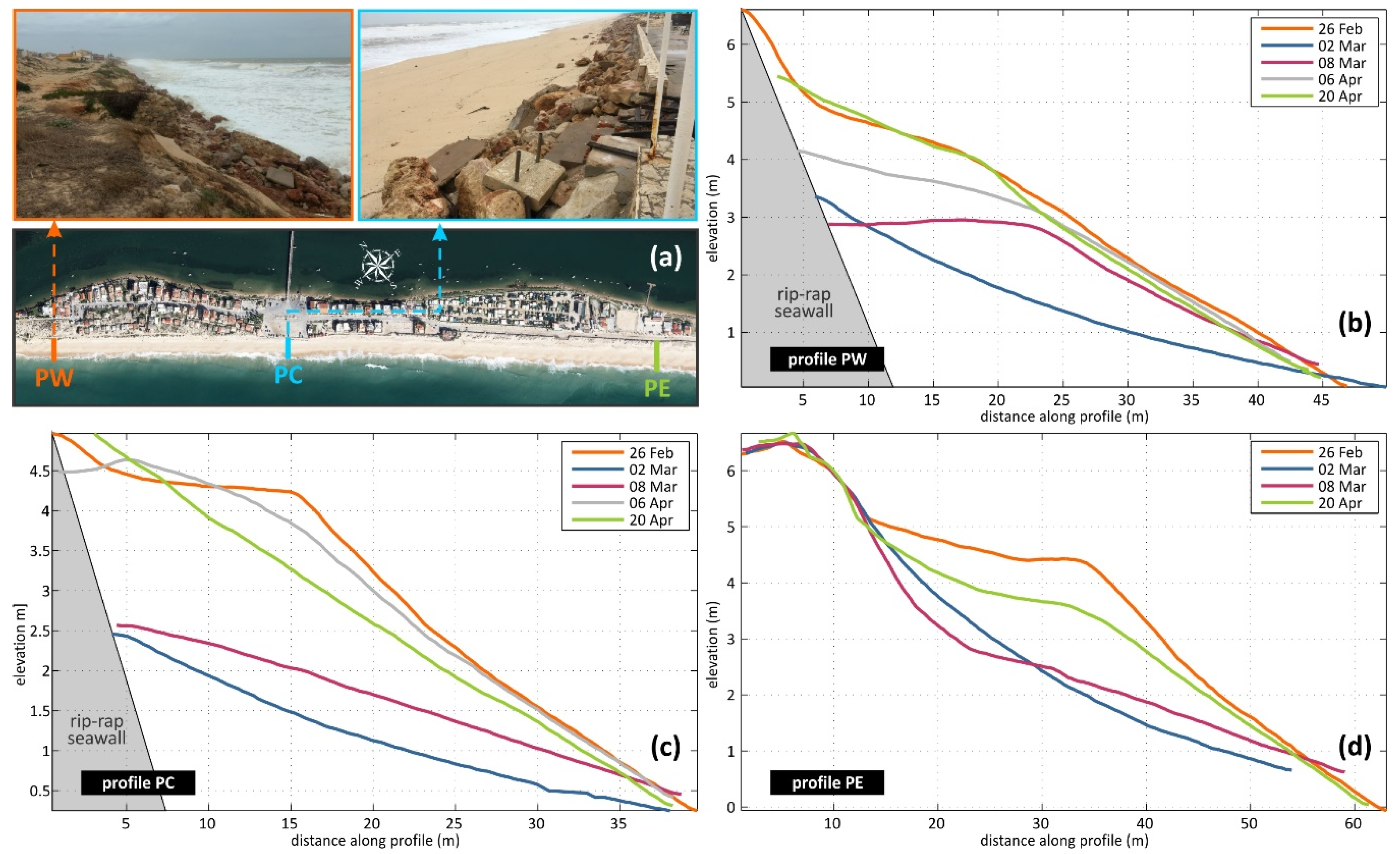
Available topographic measurements for the three profiles ([32]; Cascais vertical datum, corresponding to mean SL) are given in Figure 3 and related volume changes and beachface slopes are provided in Table 1. All profiles showed similar patterns of erosion and recovery, with intense losses right after the storm peak and high sand volume recovery until 20 April (50 days after the storm peak).
Storm-erosion volumes along the barrier stretch are similar, however alongshore differences are noted, with slightly higher values in PC (−1.68 m3/m2), followed by profile PW (−1.45 m3/m2) and minimum eroded volumes for the eastern part, in PE (−1.06 m3/m2). The higher losses in PC and PW are probably due to the low backshore widths and berm heights, compared to PE, that led to exposure of the riprap used for coastal protection (Figure 3; photos in (a) and profiles (b) and (c)). On one hand, the riprap protection had a definite stabilising effect, hindering landward retreat, but partial wave reflection on the slope is also expected to have increased erosion at the base. Pre-storm profiles were characterised by steep beachface, with slopes around 0.14–0.16 (Table 1). Directly after the storm peak the profiles showed intense “flattening” (slope at 0.05–0.06), while the recovered profiles largely returned to pre-storm steepness values.
During the first post-storm period (2 to 8 March), sand is accumulated in the lower part of the backshore (up to 2.5–3 m), which for the case of PE is combined with erosion of the upper part that reached an elevation of around 4.5 m, erosion not noted in the other two profiles due to the presence of the riprap reinforcement. In this period, profile PE was essentially readjusting, with minimal changes in volume (0.04 m3/m2), while the balance shows gains for the other two profiles (0.67 m3/m2 for PW and 0.44 m3/m2 in PC). The response of PW and PC between 8 March and 6 April is distinct (Figure 3b,c; Table 1). PC showed very intense sand accumulation, reaching elevations of 4.5 m and almost fully recovering the eroded volumes (95%), while accumulation in PW only reached levels of 4 m and a recovery of 75% of the eroded sand. The higher sand volumes in PC are due to an extraordinary, small-scale, sand replenishment in the location by the Spatial Planning Division of the Faro Municipality ([38]; personal communication) in mid-March 2018, using the sand accumulated on the roads by overwash during Emma. Unfortunately, no information is available for the characteristics of the replenished volumes and geometry, therefore the intervention could not be assimilated in the simulations. Afterwards, and until 20 April, PC was readjusting with erosion of the beachface below 4.6 m and lowering of the slope. Contrastingly, profile PW showed accretion in the zone between 3 and 5 m, with minimal changes in beachface slope. In PE, the recovery of the profile between 8 March and 20 April (no intermediate profile measurement available) includes berm development at around 3.7 m, with sand accumulation reaching 5 m within the backshore and a slightly gentler beachface, compared to pre-storm conditions. Total recovered sand volumes (8 March to 20 April) are very similar in PW and PC (1.33 and 1.31 m3/m2, respectively), with lower values for PE (0.72 m3/m2). By the end of the observation period PW, PC and PE had recovered 91.7%, 77.7% and 67.5% percent of the eroded sand, respectively, showing a tendency for slower recovery from west to east. In terms of elevation, recovery reached 5 m in all profiles.
3. Morphodynamic Modelling
3.1. Modelling Approach
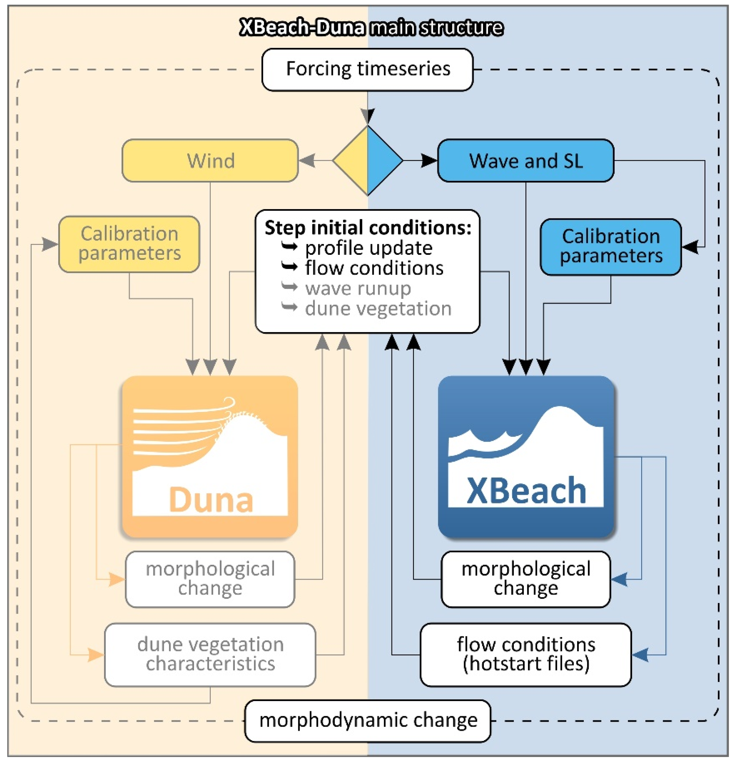
The modelling approach is based on the XBeach-Duna [39] model (Figure 4), in which the simulated period is translated into a series of marine and aeolian forcing events that trigger the corresponding module of the model. Coupling between processes is performed by updating the morphological changes of the profile after each module run and through information exchange regarding wave runup height (XBeach to Duna) and dune vegetation characteristics (Duna to XBeach). In the present work, we focus on marine processes (XBeach) and disregard aeolian morphological changes, aiming at testing the effectiveness of the approach regarding post-storm berm construction, which is the critical, first, step for profile recovery, as it provides the necessary basis of dry sediment that can lead to subsequent dune growth. This is a valid simplification for the case of the Emma storm, since, and as previously noted, even though the storm was accompanied by strong winds (9–17 m/s), aeolian transport was limited due to factors decreasing the availability of dry sand [32]. Furthermore, two of the monitored profiles (Figure 3) are constrained landwards by man-made structures and show limited (PW) or inexistent (PC) dune, while the third (PE) shows practically no change in the dune (over 5 m) between pre- and post-storm conditions, attesting to the validity of the hypothesis that the major changes in the analysed period were wave-induced.
To allow for varying calibration parameters with simulation time, XBeach (version 1.23.5526) is run in sequential steps, which in this case were set at 1 h, after the wave recording interval. To simplify the calibration process and maintain the calibrated runs as broadly applicable as possible, only two sets of fixed-value calibration parameters were considered, one for erosive and one for accretive beach response. Essentially, these conditions correspond to storm and non-storm wave incidence, which is identified from the significant wave height of each timestep (Figure 4) and assuming a storm threshold of 3 m and minimum storm duration and separation window between storms of 6 h (identified storm and non-storm conditions for the simulation period are noted on the timeline in Figure 2). Thus, the available hourly wave recordings were used to switch between the two sets of calibration parameter values and, along with SL data (also hourly), were introduced at the open boundary. A spin-up time (1 h) is considered for the first step of the loop, to allow for wave propagation to reach the beach. At the end of each step, morphological changes are used to update the profile, while flow conditions (velocities, free surface, wave energy) and suspended sediment concentrations are exported, so that they can be used for the initialisation of the next step (hotstart option; Figure 4) [40]. More details on the calibration parameters considered are given in the next Section 3.2.
3.2. Calibration Parameters
Hydrodynamics were simulated using the surfbeat (instationary) mode of XBeach that resolves short wave variations on the wave group scale and the associated long waves, while wave breaking was modelled using the time-varying dissipation rate model [41]. A morphodynamic acceleration factor (morfac; [42]) of 5 was used in the simulations, while it is noted that the sensitivity of the simulated morphologic changes compared with simulations with no morphologic acceleration was very low. The main XBeach parameters considered in the simulations are given in Table 2. Regarding boundary conditions, an absorbing-generating boundary was considered at the offshore and onshore boundaries, while input wave and SL conditions at the offshore boundary (Figure 2) were introduced as Jonswap wave-spectrum and elevation time-series, respectively. The grid step used varied between 0.5 m and 10 m for parts of the profile over the depth of 1 m and below the depth of 20 m, respectively, and non-linearly reducing steps with depth for the intermediate zone. The mean grain size was set to 0.5 mm (D50 = 0.5 mm and D90 = 0.8 mm), as characteristic for the beachface sand distribution [30]. Among the different calibration parameters tested, two were the most critical: (a) bermslope: coefficient that nudges the slope of the profile near the waterline towards its value, leading to a strong local onshore transport when the actual slope is less than the value of the coefficient [39]; and (b) facua: factor expressing the combined influence of wave skewness and asymmetry to onshore sediment transport [40].
3.3. Runup Correction
It has been established by previous works that the surfbeat mode of XBeach tends to underestimate runup, especially in steep-sloped beaches like Faro Beach, due to underestimation of the incident-band swash [44,45]. This is critical for the simulated post-storm recovery, especially regarding the upper parts of the profile, as evidenced by extensive trial calibration tests (not shown), considering various combinations of uniform, as well as time-varying facua and bermslope values. Among these, tests that accurately reproduced berm construction and the lower part of the profiles (below 3.5–4 m), were ineffective in terms of recovering sand deeper/higher into the profile, constructing a wide berm at around 3–4 m. This hints to the existence of an “elevation ceiling” for sand deposition, related to the underestimation of the runup height during the recovery phase, as the profile gradually steepens, hindering the accurate representation of the upper beachface.
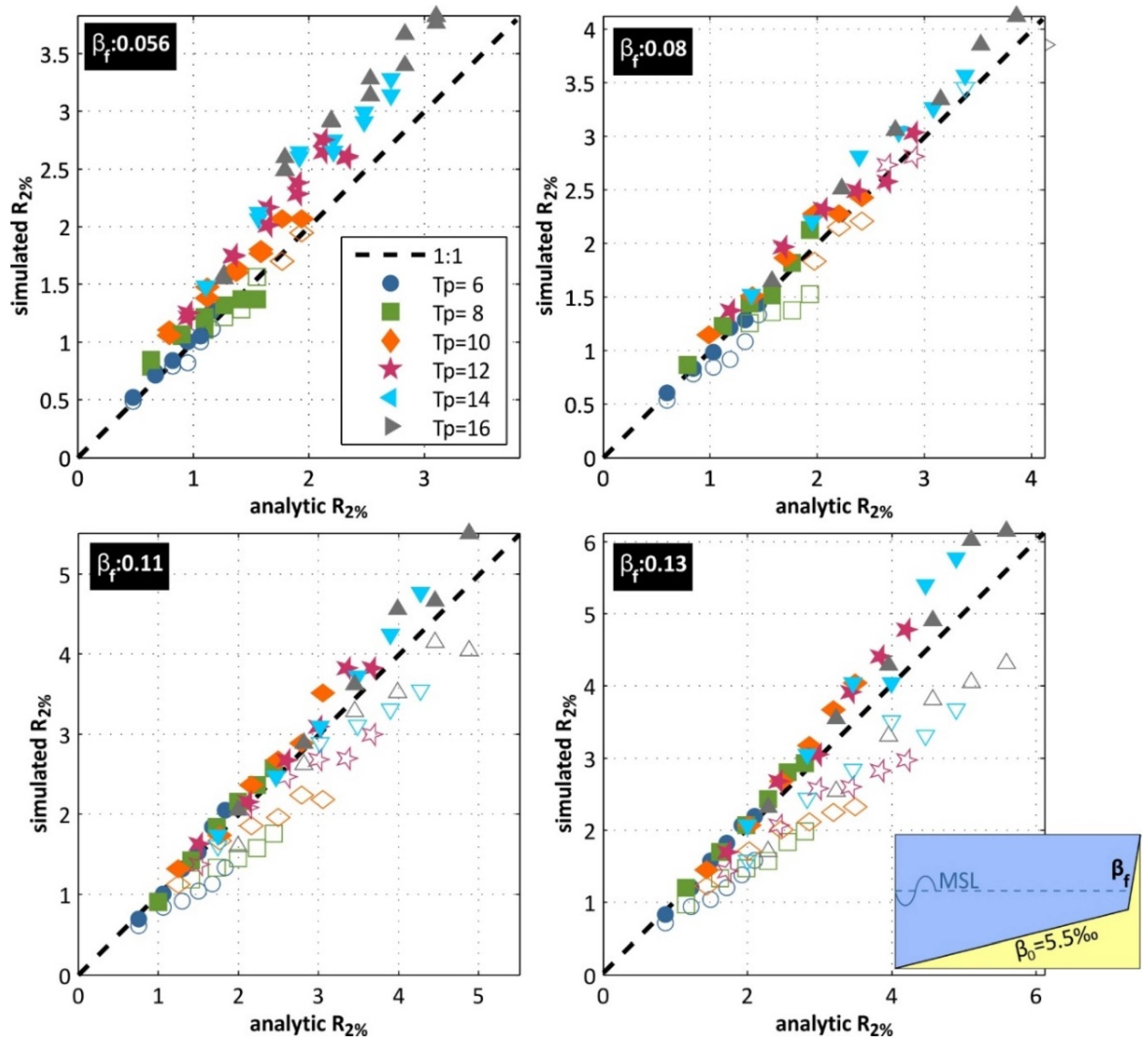
To assess this influence, a series of simplified experiments of wave incidence were conducted for an idealized bi-linear beach profile, assuming different slopes above and below the depth of 2 m (see inset sketch in Figure 5). The submerged part of the profile was set at a stable slope of 0.0055, which is the mean nearshore slope in the area, obtained by the bathymetry used in the experiments. Uniform slope value was assumed over the rest of the profile, using beachface slopes that vary within the range of values noted in the study site (βf = 0.056 to 0.13). XBeach was run for a set of variable, fixed, incident wave conditions (Hs = 1 to 6 m, with a step of 1 m; Tp = 6 to 16 s, with a step of 2 s) resolving only hydrodynamics (no change in morphology) in surfbeat mode. The R2% (2% exceedance value) runup heights were compared to the analytic expression of [46] and the results show that, as the beachface gets steeper (bf > 0.08), runup is indeed underestimated by XBeach (Figure 5; non-filled symbols). To force the runup higher into the profile, a boost in SL was applied, equal to the R2% runup height underestimation (difference between the analytic R2% value, after [46], and simulated runup; positive quantity):
The output of this runup height adjustment is given in Figure 5 (filled symbols), where the improvement of runup height approximation is clearly evidenced. It is noted the runup heights were also compared against the solution of the nonhydrostatic version of XBeach, showing improvement of the agreement after the SL boost adjustment (e.g., R2 = 0.74 versus R2 = 0.62 for βf = 0.13). This correction was applied in the model, running each sequential step of XBeach twice for the same forcing conditions (Figure 4): (a) the first time assuming only hydrodynamics, to calculate the runup on the profile morphology (assimilating the morphodynamic changes of the previous step) and; (b) the second time simulating morphodynamics and using the R2% value simulated in (a) in Equation (1) to calculate the SL boost needed to adjust the runup height. The influence to the simulated morphology of the actual profile (and the aforementioned “elevation ceiling”) can clearly be noted in Figure A1 that shows the same simulation with and without the inclusion of the runup correction (details on the calibration parameters considered are given in the next section).
4. Results
4.1. Model Calibration
Various combinations of the two calibration parameters were tested, especially regarding the accurate reproduction of the recovery phase, including time-varying values dependent on incident wave characteristics (Hs, L0, P, Hs/L0, (Hs∙L0)1/2, ξ). Even though fine-tuning of parameters can improve model accuracy, at the same time it can limit the calibrated model to a case- and site-specific solution. To balance the need for accuracy and the need for a simplistic solution, potentially applicable to other cases of steep beaches and different storms, we opted for using two sets of values for calibration parameters, one for storm and one for non-storm conditions (identified storm and non-storm conditions for the simulation period are noted on the timeline in Figure 2). The calibrated values of facua and bermslope for the three profiles are given in Table 3. For storm wave characteristics, the model considered only facua, while bermslope was switched on for non-storm waves. The latter was critical for the gradual increase of the eroded profile beachface slopes and the construction of the berm (Figure 3). Bermslope was calibrated at 0.18 for all three profiles, value slightly higher than the recovered beachface slope (0.13–0.14; Table 1). Generally high facua values were necessary, to inhibit excessive storm erosion and to recover eroded sand under non-storm conditions.
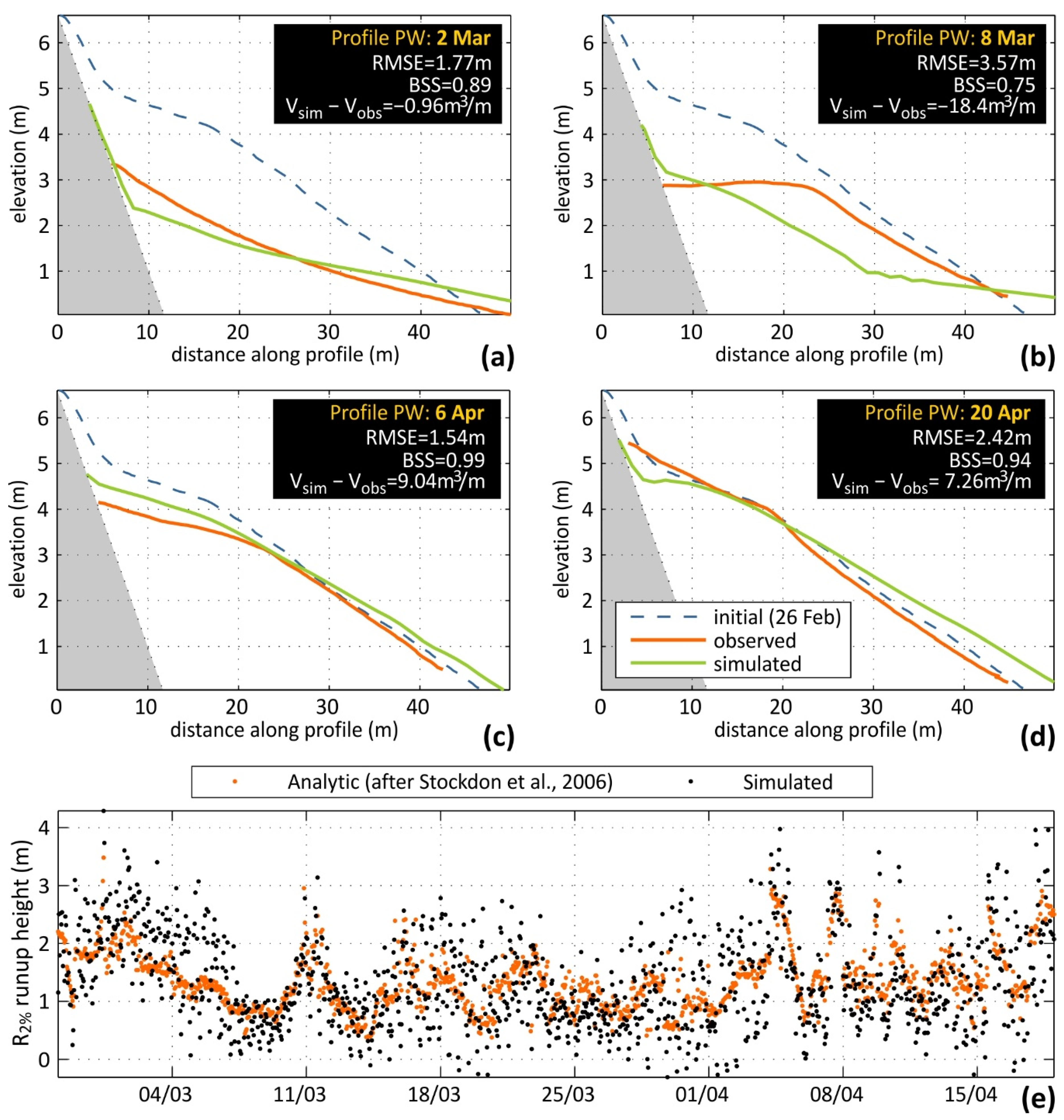
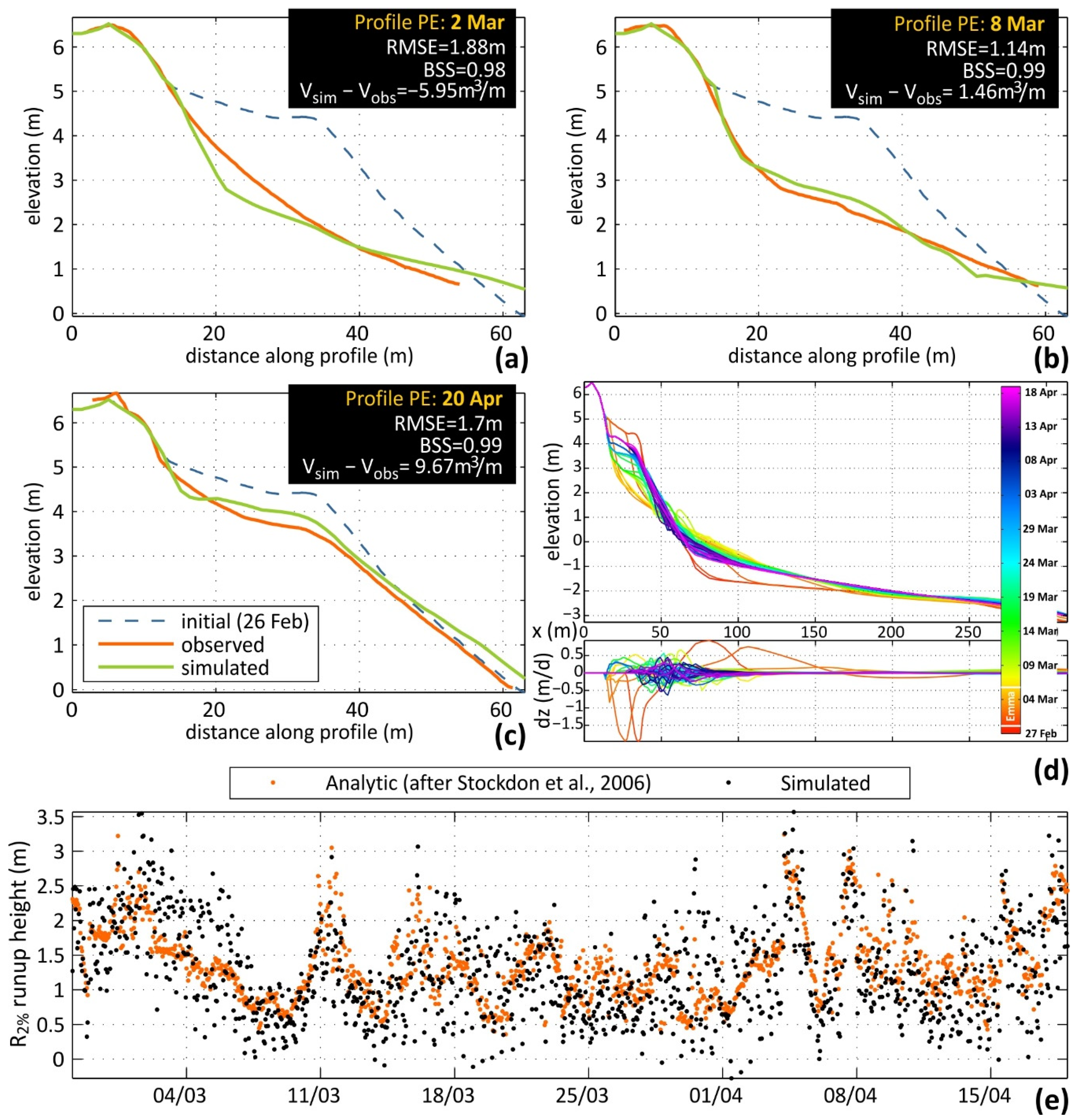
Model results for PW, PC and PE are given in Figure 6, Figure 7 and Figure 8, respectively. Goodness of fit is assessed through the Root Mean Square Error (RMSE), the Brier Skill Score (BSS; [47]) and the difference of total volume between simulation and observation (Vsim − Vobs), whose values are noted on the legend for each measured profile (also given jointly in Table 3). The lower panels in each plot (e) show the comparison between analytic values of R2% runup heights and simulated ones, after the runup correction process described in Section 3.3, showing an overall agreement between the two in all profiles.
Peak erosion (2 March) is reproduced accurately in all three profiles, with overall low RMSE between 1 and 2 m. The difference between measured and simulated volumes is near-zero (PW and PC) to very low (PE) and model error is mainly related with a slightly lower simulated beachface slope, which, for PE (Figure 8a) is combined with overestimation of erosion at the foot of the dune (not present in PW and PC due to riprap protection).
Early post-storm recovery (8 March) is not represented well by the simulation in PW (Figure 6b), with low scoring in all model evaluation indicators. The sand volumes recovered in this early stage are high, while a berm at the elevation of 3 m is already present with a very high slope (Table 1). This rapid slope recovery in PW is not shared by the other profiles, which made it difficult to formulate a uniform calibration parameter formula for entire Faro Beach test site. In fact, test runs showed that, to regain a slope of 0.11 by 8 March, non-storm parameter combinations, with distinct values than the rest of the recovery period (bermslope 0.14 and facua 0.55), needed to be applied shortly after the storm peak (1 March). However, wave forcing (Figure 2) indicates that storm conditions in the area continued until 5 March, while the same non-storm calibration parameters provided a fairly good agreement between simulation and measurement for 8 March in profile PC (Figure 7b), a profile with similar structural characteristics. Therefore, and to keep the calibration as generic as possible, the failure to reproduce the measured morphology in PW is considered acceptable, given that similar calibration values and approximation do work in the other two profiles and especially for PE that shows near-perfect agreement with the measurement (Figure 8b).
For 6 April, PW (Figure 6c) performs well, with low RMSE, perfect BSS and relatively low volume difference that shows small overestimation of recovered sand. The simulated beachface slope is slightly lower (0.118 versus 0.132) and the maximum berm height slightly higher (4.7 versus 4.1 m) than the measured ones. The related results for PC (Figure 7c) show strong underestimation of the recovered profile, especially in terms of berm height. However, as already mentioned in Section 2.3, part of the recovery of PC between 8 March and 6 April is artificial. Given that this influence was not accounted for in the simulation due to lack of data, the discrepancy between observation and simulation is expected and cannot be accounted as a failure of the calibration. The natural recovery of the profiles PC and PW should be similar and, therefore using the same parameters for the two profiles is considered appropriate.
At the end of the simulation period (April 20), the correspondence between simulation and measurement in profile PW is fairly good, with a RMSE of 2.4 m and high BSS (Figure 6d). Simulated berm slope is slightly lower (0.12 versus 0.138) and the upper part of the profile (over 4.5 m) shows lower sediment accumulation. Still, modelled recovery between 6 and 20 April did reach the elevation of 5 m, which is important in terms of effectively capturing the elevational range of the active profile within this window. For PC (Figure 7d), the approximation is very good for the part of the profile below 4 m, while the underestimation of recovered volumes is almost entirely located at the upper zone of the profile (4–5.3 m). Simulated profile PE (Figure 8c) shows good agreement with the observation, with a slight overestimation of berm height (3.8 m versus 3.6 m) and underestimation of berm slope (0.116 versus 0.127).
The approximation of runup height range and temporal variability compares well with the theoretical values, following the temporal variability and largely the range of values in all profiles. Significant peaks in the recovery period, some related to longer waves, that were underrepresented prior to the runup adjustment applied, are now captured in the simulation, decisively improving the upper range of the active profiles simulated. This can be noted in temporal evolution of simulated morphological changes, indicatively given for profile PE in Figure 8d (as profiles and bed level changes per day; top and bottom panels, respectively). The influence of the shift from the erosive calibration variable set to the accretive after the end of the storm can be easily noted, with the gradual berm formation and vertical expansion and seaward progradation. Several jumps in berm elevation can be identified, such as 16 and 30 March and 8 April, that are related to high runup levels in the preceding periods.
4.2. Model Sensitivity
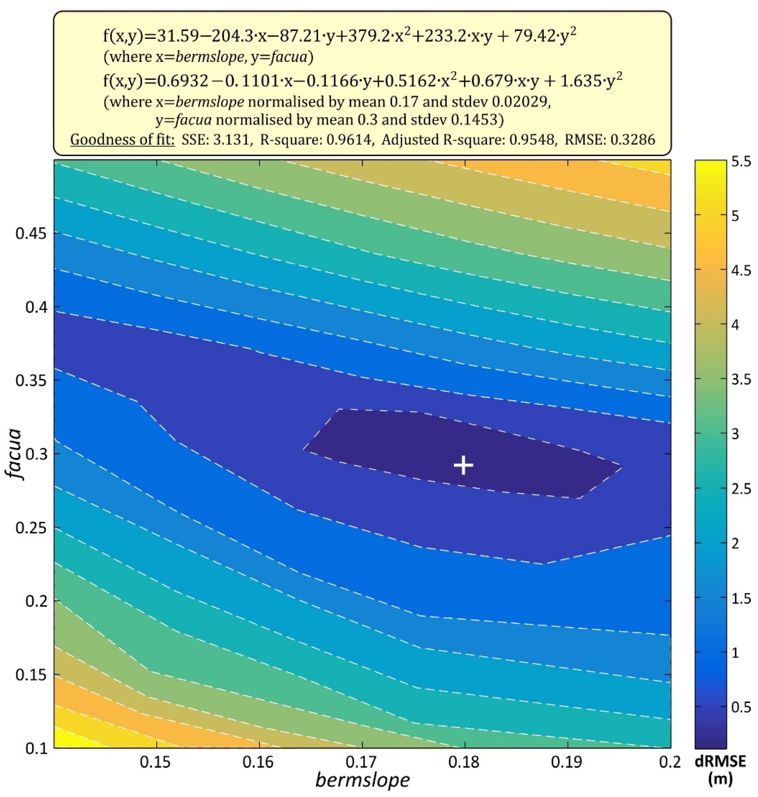
The sensitivity of the post-storm recovery (8 March to 20 April) to the selected values of the two calibration parameters was assessed by simulating a range of bermslope (0.14 to 0.2) and facua (0.1 to 0.5) combinations for profile PE. The results are presented in Figure 9 as increase of RMSE of the simulated profile, with respect to the calibration run for 20 April (Figure 8c; dRMSE). It can be noted that the increase in model error is high for both parameters (the range of facua values tested is significantly higher than the range of bermslope values), with a tendency for error maximization for low–low and high–high variable combinations (lower right and higher left parts of the plot in Figure 9). The change of dRMSE with the bermslope steps tested roughly corresponds to a rate of 0.15 m per 0.01 bermslope increase (−0.63, −0.39, −0.12, 0.07, 0.27, 0.39 and 0.46 for bermslope 0.14, 0.15, 0.16, 0.17, 018, 0.19 and 0.2, respectively). For facua, dRMSE change is around 0.16 m per 0.1 facua increase (−0.38, −0.32, −0.14, 0.29 and 0.32 for facua 0.1, 0.2, 0.3, 0.4 and 0.5, respectively).
In terms of simulated profile change with the variability of calibration parameters, the model outputs are in line with their theoretical basis. Increasing bermslope values tilt the beachface slope from milder to steeper values, with a rate close to 1:1 (e.g., increase of 0.01 in βf for increase of 0.01 in bermslope), while facua largely controls progradation of the constructed berm, at a rate of around 4.5–5 m per 0.1 facua increase. The latter value, of course, also depends on total simulation time.
5. Discussion
The calibration of XBeach in steep profiles and under low to moderate wave conditions is a challenging task, as calibrated simulations of XBeach under such conditions generally show low model skill (e.g., [48]). For calibrating the post-Emma storm recovery in Faro Beach, a crucial obstacle was the underappreciation of wave runup heights with the gradual steepening of the profile. This is a known issue of the surfbeat mode (resolving short wave groups and associated long waves) of XBeach and is mainly attributed to swash underestimation [45,49]. The nonhydrostatic version (resolving short and long waves) of XBeach performs better in terms of resolving swash and runup over a range of beach states, from reflective to dissipative [44]. However, the nonhydrostatic version of the model cannot be employed in this case, due to its high computational cost and, most importantly, to the incompatibility of sand transport formulations with the nonhydrostatic model hydrodynamics [40,50]. Therefore, surfbeat was the only viable option to model morphodynamics, thus trying to improve maximum runup heights was a necessity for capturing the recovery of Faro Beach. The SL boost employed (Equation (1)) is an indirect way to resolve the swash underestimation, that artificially forces the runup higher into the profile, without essentially correcting the swash zone width. This likely causes an upward shift to the rundown (backwash) level, as well, which we cannot assess due to lack of data. Still, the approach is similar to the one followed by [49] to assimilate swash differences between XBeach and the analytic expression of [46]. The results of the analysis performed show clear improvement both in runup predictions (Figure 5) and in induced morphological changes, attesting to the effectiveness of the approximation. The drastic improvement of simulated morphology for PE after the inclusion of the SL boost can be easily identified in Figure A1.
To the authors’ knowledge, only one previous attempt to apply a fully process-based model (XBeach) for simulating storm erosion and post-storm recovery exists, applied in the Narrabeen Beach, in Australia [51]. The results of this work showed acceptable skill and better model ability to simulate the medium-term changes to the beach profile over the annual scales than for individual storms. The present work focusses on a significantly shorter timescale compared to the Narrabeen Beach simulations and is considerably more demanding in terms of accuracy required and in terms of challenging morphological characteristics in recovery mode (higher berm heights and steeper slopes). Their approximation in calibrating separately for storm and non-storm conditions is similar to the one followed here; however, the Narrabeen Beach simulations focused over long timescales (event to annual) using statistically derived wave conditions. Even though the ultimate goal of our calibration experiments is the same, that is, calibrating XBeach for medium-term changes to allow for long-term beach-dune simulations, our approach is slightly different. Instead of passing directly to broad timesteps and statistically synthesized forcing conditions, we opted for identifying problems and verifying calibration parameters at the finest possible spatio-temporal detail, which, later on, will be used to broaden the forcing step and gradually pass on to broader timesteps.
Regarding the selected calibration parameters, the inclusion of bermslope transport term [39,52] was fundamental to the recovery of the steep slopes of Faro Beach, while balancing wave skewness and asymmetry through the facua term induced the necessary onshore sediment fluxes to balance storm erosion as well as to feed sand recovery. Distinct calibration values were necessary between profiles, even though their alongshore distances are very low. This was mainly due to the different characteristics of the profiles in terms of backshore morphology and constraints, however profile-specific calibration for individual profiles has been proven necessary to improve XBeach performance in other works (e.g., [53]). The success in calibration, while maintaining the values as broadly applied as possible, is considered important, since the experiments will be the basis for gradually reducing temporal discretization of wave climate variability, aiming at balancing model accuracy between scales (high-resolution simulations presented here and applying schematized wave forcing at an event scale). Thus, the calibration parameter fine-tuning was maintained to a minimum, considering uniform values over the entire erosion and recovery periods. This is expected to minimize the bias introduced to the simulations when repeated with a coarser temporal step in forcing, as opposed to a wave-dependant calibration value, thus facilitating the transition to event-scale simulations, as the loss of model accuracy between the analytic and event-scale simulations can be associated with the forcing schematization scheme applied.
6. Conclusions
The main conclusions, drawn from the analysis and modelling experiments presented, are summarized to the following:
- The results are novel and promising regarding the ability of a fully process-based model to reproduce post-storm recovery. XBeach performed well under challenging conditions, not only in terms of operating beyond the original model design (recovery under mild wave conditions), but also in terms of morphologic requirements of the recovered beach profiles (steep and high berms).
- The simplified approach to improve runup underestimation by the surfbeat mode of XBeach performed well for constant waves propagating on idealized beach profiles, as well as using real wave time-series and simulated morphodynamics. The related improvement of simulated beach response under mild wave conditions and steepening foreshore slopes was decisive regarding the height and shape of the recovered berm.
- Two calibration parameters were used, bermslope and facua. The former is a heuristic transport term, designed specifically to nudge the profile in the narrow area of the swash zone toward the assigned value, that was key for retrieving the steep slopes during the recovery phase. The latter is a factor that tunes the impact of wave skewness and asymmetry that allowed to enhance onshore sand transfer. The model sensitivity to the calibration parameters was, expectedly, relatively high.
- The experiments were purposefully not over-calibrated, sacrificing potential skill improvement for a generic solution, and using a set of two, fixed-value, calibration parameter groups, corresponding to destructive and constructive conditions. This will improve comparability with experiments using schematized wave forcing and allow to isolate the loss of skill introduced by the schematization.
- Building upon these results and using wave schematization techniques, we plan to formulate approaches for modelling medium-term beach morphodynamics.
Author Contributions
Conceptualization, S.C. and D.R.; methodology, S.C., D.R. and K.K.; software, D.R. and K.K.; validation, K.K. and S.C.; formal analysis, K.K. and S.C.; investigation, D.R., S.C. and K.K.; resources, S.C. and D.R.; data curation, K.K; writing—original draft preparation, K.K.; writing—review and editing, K.K., S.C. and D.R.; visualization, K.K.; supervision, S.C. and D.R.; project administration, S.C.; funding acquisition, S.C. All authors have read and agreed to the published version of the manuscript.
Funding
The work was co-financed by the European Fund for Regional Development—FEDER, through the Algarve Regional Operational Program and by National Funds, through the Foundation for Science and Technology I.P., within the scope of the ENLACE project—ALG-01-0145-FEDER-028949—PTDC/CTA-GFI/28949/2017.
Institutional Review Board Statement
Not applicable.
Informed Consent Statement
Not applicable.
Data Availability Statement
The data that support the findings of this study are available from the corresponding author upon reasonable request.
Acknowledgments
The authors would like to acknowledge the contribution of Robert McCall (Deltares, The Netherlands) to the improvement of the XBeach hotstart formulation and the financial support of the Portuguese Foundation of Science and Technology (FCT) to CIMA through UID/0350/2020.
Conflicts of Interest
The authors declare no conflict of interest.
Appendix A
Figure A1.
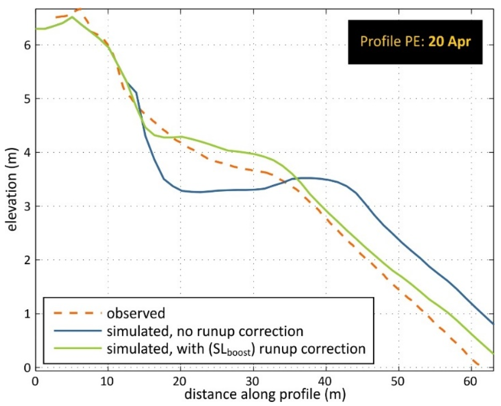
The influence of the SL boost correction to the simulated profile, shown for of PE at the end of the simulation period (20 April): Two simulated profiles (both use the calibrated values of facua and bermslope; Table 3) are shown, one with no correction for runup height (blue curve) and one after correction (SLboost; green curve–same as Figure 8c) for profile PE.
Figure A1.
The influence of the SL boost correction to the simulated profile, shown for of PE at the end of the simulation period (20 April): Two simulated profiles (both use the calibrated values of facua and bermslope; Table 3) are shown, one with no correction for runup height (blue curve) and one after correction (SLboost; green curve–same as Figure 8c) for profile PE.

References
- Karunarathna, H.; Horrillo-Caraballo, J.; Kuriyama, Y.; Mase, H.; Ranasinghe, R.; Reeve, D.E. Linkages between sediment composition, wave climate and beach profile variability at multiple timescales. Mar. Geol. 2016, 381, 194–208. [Google Scholar] [CrossRef]
- Castelle, B.; Bujan, S.; Ferreira, S.; Dodet, G. Foredune morphological changes and beach recovery from the extreme 2013/2014 winter at a high-energy sandy coast. Mar. Geol. 2017, 385, 41–55. [Google Scholar] [CrossRef]
- Toimil, A.; Losada, I.J.; Nicholls, R.J.; Dalrymple, R.A.; Stive, M.J.F. Addressing the challenges of climate change risks and adaptation in coastal areas: A review. Coast. Eng. 2020, 156, 103611. [Google Scholar] [CrossRef]
- Karunarathna, H.; Brown, J.; Chatzirodou, A.; Dissanayake, P.; Wisse, P. Multi-timescale morphological modelling of a dune-fronted sandy beach. Coast. Eng. 2018, 136, 161–171. [Google Scholar] [CrossRef]
- Fernández-Montblanc, T.; Duo, E.; Ciavola, P. Dune reconstruction and revegetation as a potential measure to decrease coastal erosion and flooding under extreme storm conditions. Ocean Coast. Manag. 2020, 188, 105075. [Google Scholar] [CrossRef]
- Scott, T.; Masselink, G.; O’Hare, T.; Saulter, A.; Poate, T.; Russell, P.; Davidson, M.; Conley, D. The extreme 2013/2014 winter storms: Beach recovery along the southwest coast of England. Mar. Geol. 2016, 382, 224–241. [Google Scholar] [CrossRef]
- Houser, C.; Wernette, P.; Rentschlar, E.; Jones, H.; Hammond, B.; Trimble, S. Post-storm beach and dune recovery: Implications for barrier island resilience. Geomorphology 2015, 234, 54–63. [Google Scholar] [CrossRef]
- Eichentopf, S.; Alsina, J.M.; Christou, M.; Kuriyama, Y.; Karunarathna, H. Storm sequencing and beach profile variability at Hasaki, Japan. Mar. Geol. 2020, 424, 106153. [Google Scholar] [CrossRef]
- Eichentopf, S.; Karunarathna, H.; Alsina, J.M. Morphodynamics of sandy beaches under the influence of storm sequences: Current research status and future needs. Water Sci. Eng. 2019, 12, 221–234. [Google Scholar] [CrossRef]
- Montreuil, A.L.; Chen, M.; Brand, E.; Verwaest, T.; Houthuys, R. Post-storm recovery assessment of urbanized versus natural sandy macro-tidal beaches and their geomorphic variability. Geomorphology 2020, 356, 107096. [Google Scholar] [CrossRef]
- Vousdoukas, M.I.; Almeida, L.P.M.; Ferreira, Ó. Beach erosion and recovery during consecutive storms at a steep-sloping, meso-tidal beach. Earth Surf. Process. Landforms 2012, 37, 583–593. [Google Scholar] [CrossRef]
- Dissanayake, P.; Brown, J.; Wisse, P.; Karunarathna, H. Effects of storm clustering on beach/dune evolution. Mar. Geol. 2015, 370, 63–75. [Google Scholar] [CrossRef]
- Ferreira, Ó.; Plomaritis, T.A.; Costas, S. Effectiveness assessment of risk reduction measures at coastal areas using a decision support system: Findings from Emma storm. Sci. Total Environ. 2019, 657, 124–135. [Google Scholar] [CrossRef] [PubMed]
- Inman, D.L.; Elwany, M.H.S.; Jenkins, S.A. Shorerise and bar-berm profiles on ocean beaches. J. Geophys. Res. 1993, 98, 18181–18199. [Google Scholar] [CrossRef]
- Bernabeu, A.M.; Medina, R.; Vidal, C. Wave reflection on natural beaches: An equilibrium beach profile model. Estuar. Coast. Shelf Sci. 2003, 57, 577–585. [Google Scholar] [CrossRef]
- Larson, M.; Kraus, N.C.; Wise, R.A. Equilibrium beach profiles under breaking and non-breaking waves. Coast. Eng. 1999, 36, 59–85. [Google Scholar] [CrossRef]
- Dodet, G.; Castelle, B.; Masselink, G.; Scott, T.; Davidson, M.; Floc’h, F.; Jackson, D.; Suanez, S. Beach recovery from extreme storm activity during the 2013-14 winter along the Atlantic coast of Europe. Earth Surf. Process. Landforms 2019, 44, 393–401. [Google Scholar] [CrossRef]
- Davidson, M.A.; Splinter, K.D.; Turner, I.L. A simple equilibrium model for predicting shoreline change. Coast. Eng. 2013, 73, 191–202. [Google Scholar] [CrossRef]
- Robinet, A.; Idier, D.; Castelle, B.; Marieu, V. A reduced-complexity shoreline change model combining longshore and cross-shore processes: The LX-Shore model. Environ. Model. Softw. 2018, 109, 1–16. [Google Scholar] [CrossRef]
- Vitousek, S.; Barnard, P.L.; Limber, P.; Erikson, L.; Cole, B. A model integrating longshore and cross-shore processes for predicting long-term shoreline response to climate change. J. Geophys. Res. Earth Surf. 2017, 122, 782–806. [Google Scholar] [CrossRef]
- Roelvink, D.; Huisman, B.; Elghandour, A.; Ghonim, M.; Reyns, J. Efficient modeling of complex sandy coastal evolution at monthly to century time scales. Front. Mar. Sci. 2020, 7, 535. [Google Scholar] [CrossRef]
- Ranasinghe, R.; Holman, R.; De Schipper, M.; Lippmann, T.; Wehof, J.; Duong, T.M.; Roelvink, D.; Stive, M. Quantifying nearshore morphological recovery time scales using ARGUS video imaging: Palm Beach, Sydney and Duck, North Carolina. Coast. Eng. Proc. 2012, 1, 24. [Google Scholar] [CrossRef]
- Robinet, A.; Castelle, B.; Idier, D.; Harley, M.D.; Splinter, K.D. Controls of local geology and cross-shore/longshore processes on embayed beach shoreline variability. Mar. Geol. 2020, 422, 106118. [Google Scholar] [CrossRef]
- Costas, S.; Ferreira, O.; Martinez, G. Why do we decide to live with risk at the coast? Ocean Coast. Manag. 2015, 118, 1–11. [Google Scholar] [CrossRef]
- Plomaritis, T.A.; Ferreira, Ó.; Costas, S. Regional assessment of storm related overwash and breaching hazards on coastal barriers. Coast. Eng. 2018, 134, 124–133. [Google Scholar] [CrossRef]
- Plomaritis, T.A.; Costas, S.; Ferreira, Ó. Use of a Bayesian Network for coastal hazards, impact and disaster risk reduction assessment at a coastal barrier (Ria Formosa, Portugal). Coast. Eng. 2018, 134, 134–147. [Google Scholar] [CrossRef]
- Dias, J.A.; Ferreira, Ó.; Matias, A.; Vila-Concejo, A.; Sá-Pires, C. Evaluation of Soft Protection Techniques in Barrier Islands by Monitoring Programs: Case Studies from Ria Formosa (Algarve-Portugal). J. Coast. Res. 2003, SI35, 117–131. [Google Scholar]
- Achab, M.; Ferreira, Ó.; Alveirinho Dias, J.M. Evaluation of sedimentological and morphological changes induced by the rehabilitation of sandy beaches from the Ria Formosa Barrier Island System (South Portugal). Thalassas 2014, 30, 21–31. [Google Scholar]
- Kombiadou, K.; Matias, A.; Ferreira, Ó.; Carrasco, A.R.; Costas, S.; Plomaritis, T. Impacts of human interventions on the evolution of the Ria Formosa barrier island system (S. Portugal). Geomorphology 2019, 343, 129–144. [Google Scholar] [CrossRef]
- Costas, S.; Ramires, M.; de Sousa, L.B.; Mendes, I.; Ferreira, O. Surficial sediment texture database for the south-western Iberian Atlantic margin. Earth Syst. Sci. Data 2018, 10, 1185–1195. [Google Scholar] [CrossRef]
- Costa, M.; Silva, R.; Vitorino, J. Contribuição para o Estudo do Clima de Agitação Marítima na Costa Portuguesa (in Portuguese). In Proceedings of the 2as Jornadas Portuguesas de Engenharia Costeira e Portuária, International Navigation Association PIANC, Sines, Portugal, 17–19 October 2001. [Google Scholar]
- Costas, S.; de Sousa, L.B.; Kombiadou, K.; Ferreira, Ó.; Plomaritis, T.A. Exploring foredune growth capacity in a coarse sandy beach. Geomorphology 2020, 371, 107435. [Google Scholar] [CrossRef]
- Oliveira, T.C.A.; Neves, M.G.; Fidalgo, R.; Esteves, R. Variability of wave parameters and Hmax/Hs relationship under storm conditions offshore the Portuguese continental coast (under revision). Ocean Eng. 2018, 153, 10–22. [Google Scholar] [CrossRef]
- Plomaritis, T.A.; Benavente, J.; Laiz, I.; Del Río, L. Variability in storm climate along the Gulf of Cadiz: The role of large scale atmospheric forcing and implications to coastal hazards. Clim. Dyn. 2015, 45, 2499–2514. [Google Scholar] [CrossRef]
- Almeida, L.P.; Ferreira, Ó.; Taborda, R. Geoprocessing tool to model beach erosion due to storms: Application to Faro beach (Portugal). J. Coast. Res. 2011, 64, 1830–1834. [Google Scholar]
- Ferreira, Ó.; Garcia, T.; Matias, A.; Taborda, R.; Dias, J.A. An integrated method for the determination of set-back lines for coastal erosion hazards on sandy shores. Cont. Shelf Res. 2006, 26, 1030–1044. [Google Scholar] [CrossRef]
- Almeida, L.P.; Ferreira, Ó.; Vousdoukas, M.I.; Dodet, G. Historical variation and trends in storminess along the Portuguese South Coast. Nat. Hazards Earth Syst. Sci. 2011, 11, 2407–2417. [Google Scholar] [CrossRef]
- Faro Municipal Council - Organization. Available online: https://www.cm-faro.pt/pt/menu/112/como-nos-organizamos.aspx#departamento-de-infraestruturas-e-urbanismo (accessed on 8 October 2020).
- Roelvink, D.; Costas, S. Coupling nearshore and aeolian processes: XBeach and Duna process-based models. Environ. Model. Softw. 2019, 115, 98–112. [Google Scholar] [CrossRef]
- Roelvink, D.; van Dongeren, A.; Mccall, R.; Hoonhout, B.; van Rooijen, A.; van Geer, P.; de Vet, L.; Nederhoff, K. Xbeach Manual; Deltares: Delft, The Netherlands, 2015. [Google Scholar]
- Roelvink, D. Dissipation in random wave groups incident on a beach. Coast. Eng. 1993, 19, 127–150. [Google Scholar] [CrossRef]
- Roelvink, J.A. Coastal morphodynamic evolution techniques. Coast. Eng. 2006, 53, 277–287. [Google Scholar] [CrossRef]
- Ruessink, B.G.; Ramaekers, G.; Van Rijn, L.C. On the parameterization of the free-stream non-linear wave orbital motion in nearshore morphodynamic models. Coast. Eng. 2012, 65, 56–63. [Google Scholar] [CrossRef]
- de Beer, A.F.; McCall, R.T.; Long, J.W.; Tissier, M.F.S.; Reniers, A.J.H.M. Simulating wave runup on an intermediate–reflective beach using a wave-resolving and a wave-averaged version of XBeach. Coast. Eng. 2020, 163, 103788. [Google Scholar] [CrossRef]
- Roelvink, D.; McCall, R.; Mehvar, S.; Nederhoff, K.; Dastgheib, A. Improving predictions of swash dynamics in XBeach: The role of groupiness and incident-band runup. Coast. Eng. 2018, 134, 103–123. [Google Scholar] [CrossRef]
- Stockdon, H.F.; Holman, R.A.; Howd, P.A.; Sallenger, A.H. Empirical parameterization of setup, swash, and runup. Coast. Eng. 2006, 53, 573–588. [Google Scholar] [CrossRef]
- Brier, G.W. Verification of Forecasts Expressed in Terms of Probability. Mon. Weather Rev. 1950, 78, 1–3. [Google Scholar] [CrossRef]
- Kalligeris, N.; Smit, P.B.; Ludka, B.C.; Guza, R.T.; Gallien, T.W. Calibration and assessment of process-based numerical models for beach profile evolution in southern California. Coast. Eng. 2020, 158, 103650. [Google Scholar] [CrossRef]
- Stockdon, H.F.; Thompson, D.M.; Plant, N.G.; Long, J.W. Evaluation of wave runup predictions from numerical and parametric models. Coast. Eng. 2014, 92, 1–11. [Google Scholar] [CrossRef]
- Jongedijk, C.E. Improving XBeach Non-Hydrostatic Model Predictions of the Swash Morphodynamics of Intermediate-Reflective Beaches. Master’s Thesis, Delft University of Technology, Delft, The Netherlands, 2017. [Google Scholar]
- Pender, D.; Karunarathna, H. A statistical-process based approach for modelling beach profile variability. Coast. Eng. 2013, 81, 19–29. [Google Scholar] [CrossRef]
- Roelvink, D.; McCall, R.; Costas, S.; Van Der Lugt, M. Controlling swash zone slope is key to beach profile modelling. In Proceedings of the 9th International Conference Coastal Sediments 2019, Tampa/St. Petersburg, FL, USA, 27–31 May 2019; Wang, P., Rosati, J.D., Vallee, M., Eds.; World Scientific Publishing Co. Pte. Ltd.: Singapore, 2019; pp. 149–157. [Google Scholar]
- Simmons, J.A.; Splinter, K.D.; Harley, M.D.; Turner, I.L. Calibration data requirements for modelling subaerial beach storm erosion. Coast. Eng. 2019, 152, 103507. [Google Scholar] [CrossRef]
Figure 1.
Location of Faro Beach (Praia de Faro) in the Ria Formosa system (top; Faro buoy is indicated in the image and the location of Ria Formosa and of the Huelva tidal gauge station are noted on the map, to the right) and of the 3 monitored profiles, PW, PC and PE (bottom).
Figure 1.
Location of Faro Beach (Praia de Faro) in the Ria Formosa system (top; Faro buoy is indicated in the image and the location of Ria Formosa and of the Huelva tidal gauge station are noted on the map, to the right) and of the 3 monitored profiles, PW, PC and PE (bottom).

Figure 2.
Time-series of significant wave height (Hs) and Sea Level (SL) (a), wave peak period (Tp; b) and onshore wave direction (θp,onshore, with positive values denoting waves directed toward the inlet; c). Wave data were collected from the Faro buoy (located at a depth of 93 m; Figure 1). Sea levels refer to surge levels (Huelva tide gauge) and astronomical tides for Faro. The yellow-shaded area on the plots denotes the incidence of Emma storm (28 February–5 March), green arrows show the dates of profile measurement and identified storm and non-storm conditions are marked (orange and blue, respectively) on the timeline above (a).

Figure 3.
Location of profiles and photos of post-storm beach conditions (PW and PC) (a) and measured pre-storm (26 February), post-storm (2 and 8 March) and recovered (6 and 20 April) profiles for PW (b), PC (c) and PE (d; no measurement is available for 6 April). Elevations are relative to mean SL (Cascais vertical datum).

Figure 4.
The coupled XBeach-Duna modelling approach: the left panel presents aeolian processes (disabled for the case of the Emma run) and the right panel shows marine processes and flow of inputs and outputs.
Figure 4.
The coupled XBeach-Duna modelling approach: the left panel presents aeolian processes (disabled for the case of the Emma run) and the right panel shows marine processes and flow of inputs and outputs.

Figure 5.
Comparison of analytic R2% runup heights, calculated after [46], and simulated values before (non-filled symbols) and after correction (filled symbols) for different beachface slopes (βf = 0.056, 0.08, 0.11 & 0.13) and incident waves (Tp = 6–16 s, noted on the legend, and Hs =1, 2, 3, 4, 5 & 6 m). The correction (SL boost) was applied only when R2% was underestimated by XBeach, otherwise both runs have the same simulated R2% value (filled and non-filled symbols overlap). A sketch of the idealized profile, used, is given in the lower-right panel.

Figure 6.
Calibration results for profile PW (see Figure 1 for location): (a–d) show the goodness of fit between simulated (green line) and observed (orange line) profiles for 2 and 8 March and 6 and 20 April, respectively (RMSE, BSS and total volume difference between simulation and observation (Vsim − Vobs) are given in the legend); the time-series of theoretic (orange dots, after [46]) and simulated (black dots) R2% runup heights are given in (e).

Figure 7.
Calibration results for profile PC (see Figure 1 for location): (a–d) show the goodness of fit between simulated (green line) and observed (orange line) profiles for 2 and 8 March and 6 and 20 April, respectively (RMSE, BSS and total volume difference between simulation and observation (Vsim − Vobs) are given in the legend); the time-series of theoretic (orange dots, after [46]) and simulated (black dots) R2% runup heights are given in (e).

Figure 8.
Calibration results for profile PE (see Figure 1 for location): (a–c) show the goodness of fit between simulated (green line) and observed (orange line) profiles for 2 and 8 March and 20 April, respectively (RMSE, BSS and total volume difference between simulation and observation (Vsim − Vobs) are given in the legend); (d) shows profile changes (top panel) and alongshore elevation change rates (in m/d; bottom panel) with time (color bar; the Emma storm duration is noted); the time-series of theoretic (orange dots, after [46]) and simulated (black dots) are given in (e).

Figure 9.
Increase of RMSE (dRMSE in m; color-scale) with bermslope and facua with respect to the calibration run (cross); all combinations were simulated for profile PE and the recovery period (8 March to 20 April) and the dRMSE values shown refer to the end of the simulation (20 April). A second order polynomial equation is fitted to the values (on top).


Table 1.
Volume changes (top panel; values in parentheses refer to m3/m per m of profile) and beachface slopes (bottom panel) for the three profiles. Volume changes are given for the erosion phase (26 February to 2 March) and for the recovery period, as a whole (2 March to 20 April), and analyzed in differences between consecutive measured profiles (6 April not measured in PE; the value refers to 8 Mar to 20 April). For consistency, only profile stretches present in all monitored profiles were used for volume calculation (profile lengths of 35.9, 33.8 and 51.2 m for PW, PC and PE, respectively).
| Profile | ||||
|---|---|---|---|---|
| Period/Date | PW | PC | PE | |
| Volume change {m3/m (m3/m2)} | 26 February to 2 March | −52.21 (−1.45) | −56.82 (−1.68) | −54.32 (−1.06) |
| 2 March to 20 April | 47.86 (1.33) | 44.16 (1.31) | 36.67 (0.72) | |
| 2 March to 8 March | 24.17 (0.67) | 14.85 (0.44) | 2.19 (0.04) | |
| 8 March to 6 April | 15.23 (0.42) | 38.99 (1.15) | 34.48 (0.67) | |
| 6 April to 20 April | 8.46 (0.24) | −9.68 (−0.29) | ||
| Beachface slope, βf (%) | 26 February | 13.7 | 16.1 | 15.2 |
| 2 March | 5.6 | 5.0 | 6.4 | |
| 8 March | 11.0 | 6.7 | 6.6 | |
| 6 April | 13.2 | 14.7 | - | |
| 20 April | 13.8 | 12.6 | 13.3 | |
Table 2.
Simulation/calibration parameters.
| XBeach Parameters | ||
|---|---|---|
| Name | Description | Parameterization/Value |
| break | wave breaking formulation | roelvink2 [41] |
| gamma | breaker parameter | 0.55 |
| gammax | maximum ratio wave height to water depth | 0.2 |
| maxbrsteep | maximum wave steepness criterium | 0.3 |
| waveform | wave shape model | ruessink_vanrijn [43] |
| turb | turbulence variance at the bed | wave_averaged |
| bedfriction | bed friction formulation | manning |
| bedfriccoef | bed friction coefficient (manning n) | 0.025 for sand 0.05 over riprap wall |
| facua | calibration factor for time averaged flows due to wave skewness and asymmetry | variable |
| bermslope | calibration factor for swash zone slope | variable (~βf) |
Table 3.
Calibration parameters (storms correspond to Hs ≥ 3 m) and related goodness of fit indicators for the 3 profiles (PW, PC and PE).
Table 3.
Calibration parameters (storms correspond to Hs ≥ 3 m) and related goodness of fit indicators for the 3 profiles (PW, PC and PE).
| Calibration Parameters | PW | PC | PE | |
|---|---|---|---|---|
| storm | facua | 0.75 | 0.65 | 0.75 |
| non-storm | bermslope | 0.18 | 0.18 | 0.18 |
| facua | 0.4 | 0.4 | 0.28 | |
| goodness of fit | ||||
| RMSE (m) | 02 Mar | 1.77 | 0.99 | 1.88 |
| 08 Mar | 3.57 | 2.39 | 1.14 | |
| 06 Apr | 1.54 | 3.45 | no data | |
| 20 Apr | 0.94 | 1.18 | 1.7 | |
| Vsim − Vobs (m3/m) | 02 Mar | −0.96 | −0.18 | −5.95 |
| 08 Mar | −18.4 | 0.79 | 1.14 | |
| 06 Apr | 9.04 | 3.45 | no data | |
| 20 Apr | 7.26 | −3.97 | 9.67 | |
Publisher’s Note: MDPI stays neutral with regard to jurisdictional claims in published maps and institutional affiliations. |
© 2021 by the authors. Licensee MDPI, Basel, Switzerland. This article is an open access article distributed under the terms and conditions of the Creative Commons Attribution (CC BY) license (http://creativecommons.org/licenses/by/4.0/).
Share and Cite
MDPI and ACS Style
Kombiadou, K.; Costas, S.; Roelvink, D. Simulating Destructive and Constructive Morphodynamic Processes in Steep Beaches. J. Mar. Sci. Eng. 2021, 9, 86. https://0-doi-org.brum.beds.ac.uk/10.3390/jmse9010086
AMA Style
Kombiadou K, Costas S, Roelvink D. Simulating Destructive and Constructive Morphodynamic Processes in Steep Beaches. Journal of Marine Science and Engineering. 2021; 9(1):86. https://0-doi-org.brum.beds.ac.uk/10.3390/jmse9010086
Chicago/Turabian StyleKombiadou, Katerina, Susana Costas, and Dano Roelvink. 2021. "Simulating Destructive and Constructive Morphodynamic Processes in Steep Beaches" Journal of Marine Science and Engineering 9, no. 1: 86. https://0-doi-org.brum.beds.ac.uk/10.3390/jmse9010086
Note that from the first issue of 2016, this journal uses article numbers instead of page numbers. See further details here.