Article

Study on Reactive Power Compensation Strategies for Long Distance Submarine Cables Considering Electrothermal Coordination

1
School of Electric Power Engineering, South China University of Technology, Guangzhou 510640, China
2
China Energy Engineering Group Guangdong Electric Power Design Institute Co., Ltd., Guangzhou 510663, China
*
Author to whom correspondence should be addressed.
J. Mar. Sci. Eng. 2021, 9(1), 90; https://0-doi-org.brum.beds.ac.uk/10.3390/jmse9010090
Submission received: 17 December 2020 / Revised: 10 January 2021 / Accepted: 12 January 2021 / Published: 15 January 2021

Abstract

:
Long-distance high voltage alternating current (AC) submarine cables are widely used to connect offshore wind farms and land power grids. However, the transmission capacity of the submarine cable is limited by the capacitive charging current. This paper analyzes the impacts of reactive power compensation in different positions on the current distribution on long-distance submarine cable transmission lines, and tests the rationality of the existing reactive power compensation schemes based on electrothermal coordination (ETC). Research shows that compensation at the sending end has obvious impacts on current distribution along the cable, and the maximum current occurs at the sending or receiving end. Moreover, the reactive power compensation at sending end will reduce the current at receiving end of the line. On the contrary, it will increase the current at sending end. Compared with the directly buried laying method of the submarine cable in the landing section, the cable trench laying method can increase the cable ampacity of the landing section and reduce the reactive power compensation capacity at the sending end. The ampacity is the current representation of the thermal limits of the cable. ETC exploits the cable ampacity to coordinate current distribution on transmission lines under existing reactive power compensation schemes, thus optimizing the reactive power compensation schemes and avoiding the bottleneck point of cable ampacity.

1. Introduction

Wind energy, as an efficient clean energy, has been increasingly valued. The utilization of wind energy to generate electricity can enrich energy supply systems and reduce environment pollution. In Europe, there were 3412 MW of installed capacity being increased, and about 500 wind turbines were installed in 2019, making Europe the world leader in the development of offshore wind power [1]. Compared with Europe, the wind power has been developing rapidly in China in recent years. The wind power generation in 2019 was 405.7 billion kW·h, accounting for 5.5% of total power generation [2]. Compared with the onshore wind power generation, the offshore wind power is rich in resources and has great development potential. The advantages of wind power in offshore wind farms, such as high wind speed, being more stable, and having less impact on the environment, etc., are attracting attention from more and more countries.
High-voltage AC cable and high-voltage direct current (DC) cable are commonly used in offshore wind power transmission lines. High voltage AC transmission has the advantages of simple structure and low cost. When the transmission distance is long, the transmission capacity of high-voltage AC cables is greatly affected by the charging current, and the loss caused by reactive power exchange will be more obvious [3,4]. The transmission capacity of high-voltage DC cable is large, and the loss is low. However, the construction and operation costs are high, requiring building offshore and onshore converter stations [5]. These disadvantages have motivated some researches to look for methods to extend the feasibility of the high-voltage AC cable alternative.
Aiming at the losses problem caused by the transmission system of high-voltage AC submarine cables in offshore wind farms, there are two common methods. One is to change the mode of system operation: To use lower operating frequency or to change the transmission voltage to reduce losses. In 2017, Gustavsen and Mo [6] proposed to improve the transmission capacity of the submarine cables by continuously changing the operating voltage of the long-distance submarine cables according to the output power of the wind farm. Using a lower frequency (less than the standard 50/60 Hz) to reduce the charging current on the transmission line and the skin effect on the conductor surface was analyzed in Ref. [7]. Another alternative is to consider using external equipment to compensate reactive power to reduce reactive current. The reactive power compensation plans for submarine cable transmission lines mainly include the single-terminal compensation, the two-terminal compensation, and the middle line compensation, also the configuration scheme considering the comprehensive utilization of the reactive power output capacity of wind turbines. The middle line compensation of submarine cable transmission lines was considered by Gatta in 2011 [8]. Abram and Ola [9] designed the reactive power allocation plan of offshore wind farm transmission systems based on the reactive power capacity of wind turbines themselves and the high resistance of power grid side. In general, regarding the requirements of reactive power exchange and reactive power compensation strategies, different rules have been set in some European countries, Denmark, Germany, and Britain, which rule power factors of interconnection point within a certain range [10,11,12]. These rules are more considered from the point of view of transmission system operation, but the impacts of reactive power compensation strategies on current on the transmission line is seldom considered. Under the condition of satisfying the steady operation of the system, the thermal limits of long-distance submarine cables are also an important problem.
The output submarine cables of offshore wind farms will pass through different laying sections, relating to various laying environments. Therefore, the steady-state ampacity of each laying section may vary greatly [13]. The current research is mainly focused on considering more environmental factors and establishing more accurate models to calculate the cable ampacity of submarine cables [14,15,16,17,18]. However, long-distance submarine cables are also affected by charging current. The reactive power compensation can improve the transmission power factors and it also changes the current distribution on the submarine cable transmission line [19]. For some laying sections with poor heat dissipation condition, when the wind farm is fully loaded or overloaded, some submarine cable sections may overheat to accelerate the aging of submarine cable insulation [20,21].
In this paper, an accurate PI equivalent model is used to calculate the current distribution in the long-distance submarine cable transmission line. Based on this model, impacts of various reactive power compensation schemes on the current distribution in the transmission line is analyzed and simulated. Then, the ampacity of the long-distance submarine cable is calculated under different laying methods based on IEC60287 standard [22]. Research tested the rationality of the existing reactive power compensation schemes from the point of view of electrothermal coordination (ETC) [23,24]. Cable ampacity is the current representation of the cable thermal limits. The ETC approach for system operation is compatible with and can determine more reasonable reactive power compensation schemes. It can avoid the occurrence of ampacity bottlenecks and provide a reference for the reactive power compensation schemes of the offshore wind farm output cables.

2. Electrical Calculation Model of HVAC Cables in Offshore Wind Farm

2.1. Structure of Offshore Wind Power System

The offshore wind power generation system based on high-voltage AC transmission is shown in Figure 1. It mainly consists of three parts: The first one is the offshore wind turbine generator, and its function is to use the rotation of wind turbines to generate electricity. The second part is the transformation part. The generated electric energy is concentrated through the array cables, and then the voltage is raised by the offshore booster station. The third part is the transmission part, where the electricity raised by the offshore booster station is finally transmitted to the onshore terminal of the landing point through the long-distance submarine cables. As the offshore wind farms are generally built in the ocean areas far from the coast, the charging power per unit length of submarine cable is very large, which will cause a large charging current on the submarine cables and restrict the transmission capacity of the whole wind farm system [25]. According to literature [26], the wind farms should meet the requirements of being able to arrange the active power output and the reactive power output. Therefore, for offshore wind farms, the reactive power compensation is carried out at the offshore booster stations and the onshore centralized control center based on the principles of section dividing and local balance of reactive power compensation, and reactive power compensation equipment such as reactor, SVC, or STATCOM are usually installed [10,27].

2.2. Cable Design and Characteristics

The structure of high-voltage submarine cable can be divided into the single-core and the three-core. Compared with the single-core structure, the three-core submarine cable has less loss and low laying cost. With the maturity of manufacturing technology, the three-core high-voltage submarine cable has been applied increasingly to the trans-sea power transmission [28]. A simplified cross section drawing of a typical three-core submarine cable is shown in the Figure 2.
The high-voltage AC submarine cable consists of three cores and outer material. The wire core materials from inside to outside successively are water-blocking copper conductor stranded by copper wires, conductor screen, cross-linked polyethene (XLPE) insulating layer, insulating screen, swelling tape, lead alloy sheath, anti-corrosion sheath, and filling layer. The outer materials from inside to outside successively are bedding, armor layer, and outer serving. In the filling layer, fiber optic units are usually distributed as channels for wind farm communication and submarine cable monitoring signal. The main structure parameters of the 220 kV, 3 × 500 mm2 three-core submarine cable are shown in Table 1.

2.3. Lumped Parameter Model of Submarine Cables

Due to the influence of charging current, problems such as overcurrent and overvoltage will occur on the long-distance submarine cables, which will affect the safe operation of lines. To calculate the value of current, voltage, and power on the submarine cable line, a suitable cable model should be selected. The accuracy and complexity of the model are two indexes that often need to be concerned. The models of submarine cables mainly include the PI-type equivalent model of lumped parameters and the Bergeron model and frequency-dependent model of distributed parameters; the Bergeron model ignores the series impedance and admittance of the cable line. The line is considered as a lossless line, and the overall loss of line is considered only at both ends of the line; the frequency-dependent model is applied for the transient overvoltage analysis and the harmonic analysis [19]. According to [19], in the field of steady-state analysis of power systems, choosing to use complex cable models cannot improve the accuracy of the problems analyzed. Therefore, the accurate PI equivalent circuit model is considered in this paper, as shown in Figure 3.
Where, R is the resistance of the circuit, Ω; L is the inductance of the circuit, H; G is the conductance of the circuit, S; C is capacitance, F. The above parameters are calculated by Carson–Clem formula [29], as shown in Table 2. The impedance and admittance of the submarine cable PI equivalent circuit are respectively represented by Z and Y.
Z ω = R + j ω L
Y ω = G / 2 + j ω C / 2
According to literature [30], the relationship between voltage and current at the sending and receiving ends of the line is shown as follows:
V ˙ s 1 I ˙ s 1 = cosh γ l + Z c Y 2 sinh γ l Z c sinh γ l 1 Z c + Z c Y 1 Y 2 sinh γ l + ( Y 1 + Y 2 ) cosh γ l cosh γ l + Z c Y 1 sinh γ l V ˙ r 1 I ˙ r 1
where Y1 and Y2 represent equivalent susceptance of inductors installed at the sending and receiving ends of HVAC cable for compensation; Vs1, Vr1 and Is1, Ir1, respectively represent the voltage and current at sending and receiving ends of line; l is the length of the line; γ is the transmission coefficient of line; and Zc is the characteristic impedance of the line.
Z c ω = Z ω Y ω
γ ω = Z ω Y ω
In order to accurately calculate the current and voltage at each point along the line, in literature [6], the transmission line of long-distance submarine cable is evenly divided into N segments of PI equivalent circuits, then the length of each section is Lseg = L/N, as shown in Figure 4. In Figure 4, V1, V2...Vn+1 and I1, I2...In+1 are respectively representing the voltage and current value of each PI equivalent circuit connection node from the sending end to the receiving end.
According to literature [31], in this paper, each section is considered as 1 km. For a submarine cable with L km length, it will be divided into L sections of PI equivalent circuit. The node analysis method is used to calculate the voltage and current value on each node in MATLAB, as shown in Figure 5.
In Figure 5, Vs and Vr are the voltage values at sending and receiving ends respectively; IS and Ir are respectively the input and output current values at sending and receiving ends; QS, Qr, and Qm are for the reactive compensation power capacity at the sending end, receiving end, and middle line, respectively. According to Figure 5, the mathematical model in MATLAB for solving the line current distribution is shown as below. In this part, taking the reactive power compensation at 1/2 of long-distance submarine cables as an example to show the mathematic model.
For sending end:
I s = P / 3 V 1 cos φ 1 I ˙ 0 = V ˙ 1 / i * V 1 2 / Q s I ˙ 1 = I ˙ s I ˙ 0 I ˙ y 1 = V ˙ 1 Y I ˙ z 1 = I ˙ 1 I ˙ y 1 V ˙ 2 = V ˙ 1 I ˙ z 1 Z
For middle line:
V ˙ n / 2 + 1 = V ˙ n / 2 I ˙ z n / 2 Z I ˙ y n / 2 + 1 = V ˙ n / 2 + 1 Y I ˙ m = V ˙ n / 2 + 1 / i * V n / 2 + 1 2 / Q m I ˙ n / 2 + 1 = I ˙ z n / 2 I ˙ y ( n / 2 + 1 ) I ˙ m I ˙ z n / 2 + 1 = I ˙ n / 2 + 1 I ˙ y n / 2 + 1
For receiving end:
V ˙ n + 1 = V ˙ n I ˙ z n Z I ˙ y n + 1 = V ˙ n + 1 Y I ˙ d = V ˙ n + 1 / i * V n + 1 2 / Q r I ˙ n + 1 = I ˙ z n I ˙ y ( n + 1 ) I ˙ r = I ˙ n + 1 I ˙ d
where P is the active power transmitted by the submarine cable line, I0, Im, and Id is the current of reactive power compensation equipment on the sending, middle line, and receiving end, respectively, Iy1Iyn and Iz1Izn are respectively representing the current of admittance and impedance of PI equivalent circuit, cosφ1 is the transmission power factors of the sending end of the submarine cable line, and i is the unit of imaginary number.

3. Impacts of Reactive Power Compensation on Current Distribution of for Long-Distance Submarine Cables

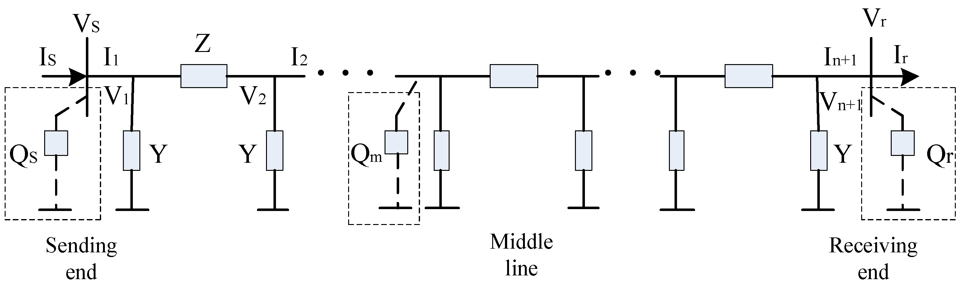
Due to the large capacitance of high-voltage submarine cables, plenty of reactive power will be generated. The reactive compensation is usually adopted to solve this problem. Because of the limitation of engineering conditions, the reactive compensation for the submarine cables cannot be conducted along the line, but can only be conducted centrally at both ends of the line or on the land halfway [27]. The influence of different reactive power compensation schemes on the current distribution of submarine cables is analyzed in detail below.
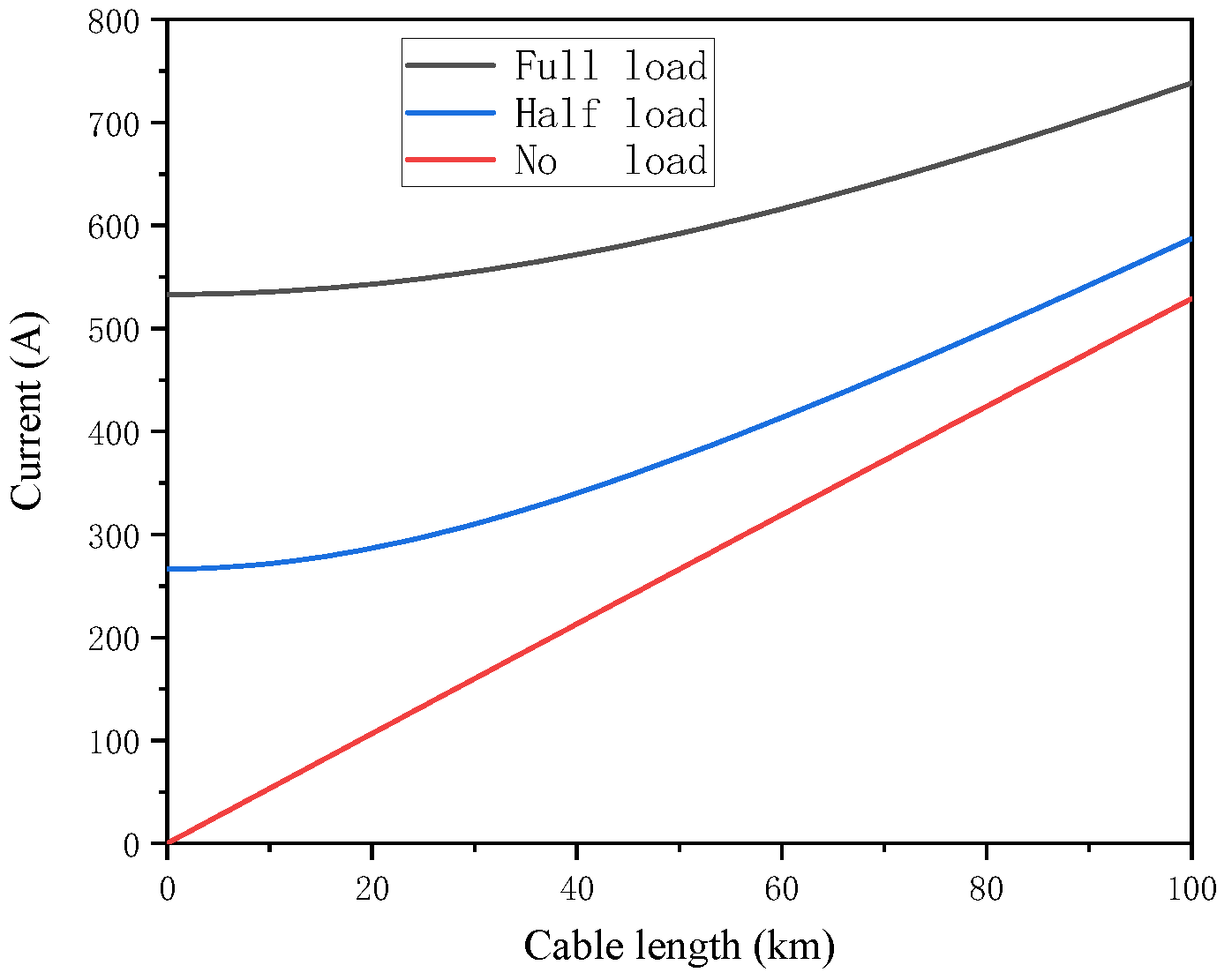
Assuming that the rated voltage of long-distance submarine cable lines is 220 kV, the voltage at the sending end of the submarine cable transmission is 1.05 times of the rated voltage, as 232 kV, and the full load state will be the moment when the transmission power reaches 203.5 MW. As shown in Figure 6, under no-load condition, the charging current distribution on the line has a linear relationship with the transmission distance. The farther the transmission distance is, the larger the current on the line will be. When the submarine cable line is half-loaded or fully loaded, the current at the receiving end of the line is much larger than that at the sending end of the line due to the large charging current of the cable without reactive compensation. For a 100 km submarine cable transmission line, the current at the line terminal reaches 220% and 138% of the current at sending end respectively under half-load and full load conditions. For some laying sections with poor heat dissipation conditions, the current on the submarine cable line may exceed its ampacity when the load is high, causing the cable overheated operation, which will accelerate the aging of the cable insulation and reduce the service life of the cable.
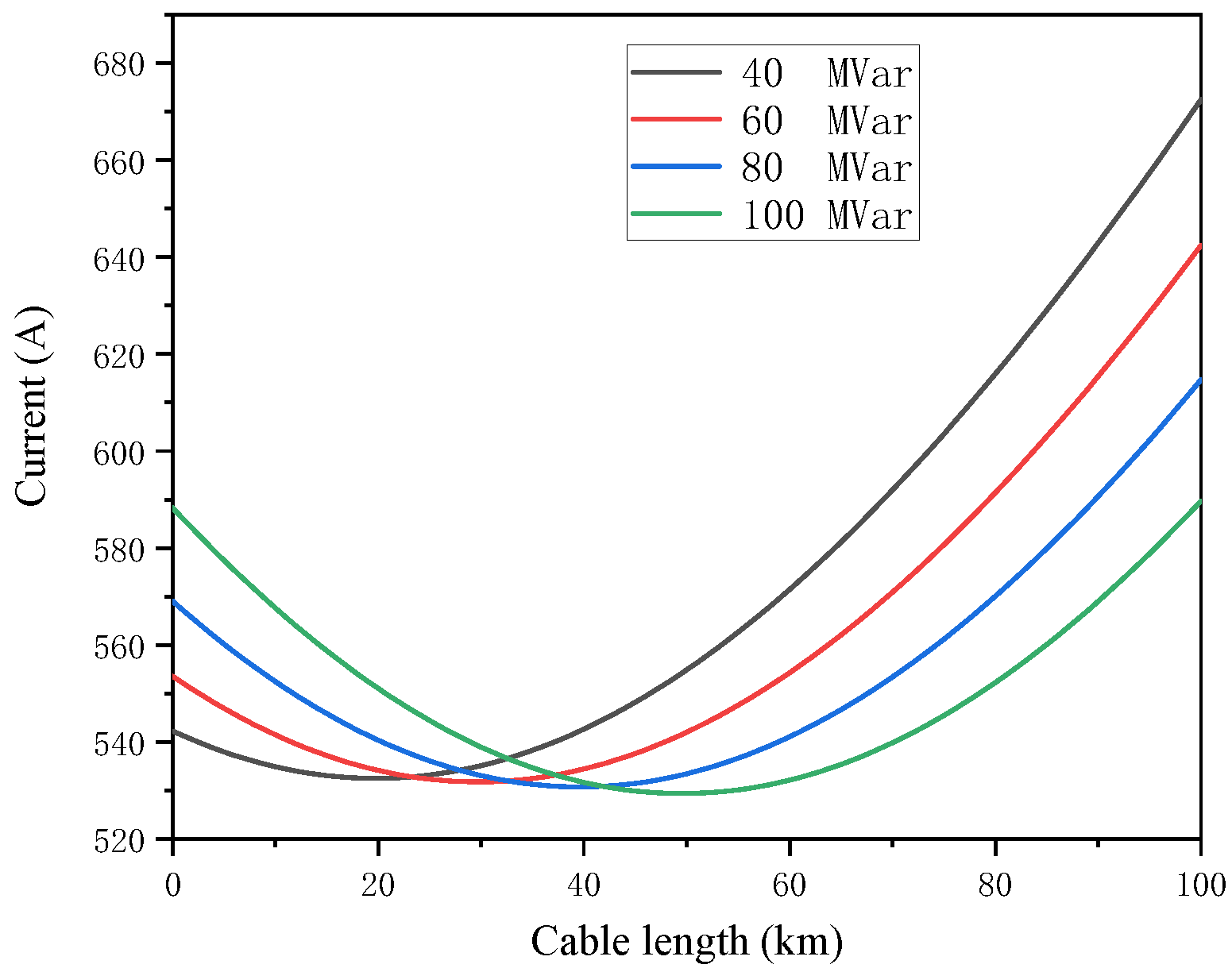
In order to analyze the influence of the different shunt compensation locations on the line current, the reactive compensations are conducted respectively to the sending end and receiving end of a certain length submarine cable line. As shown in
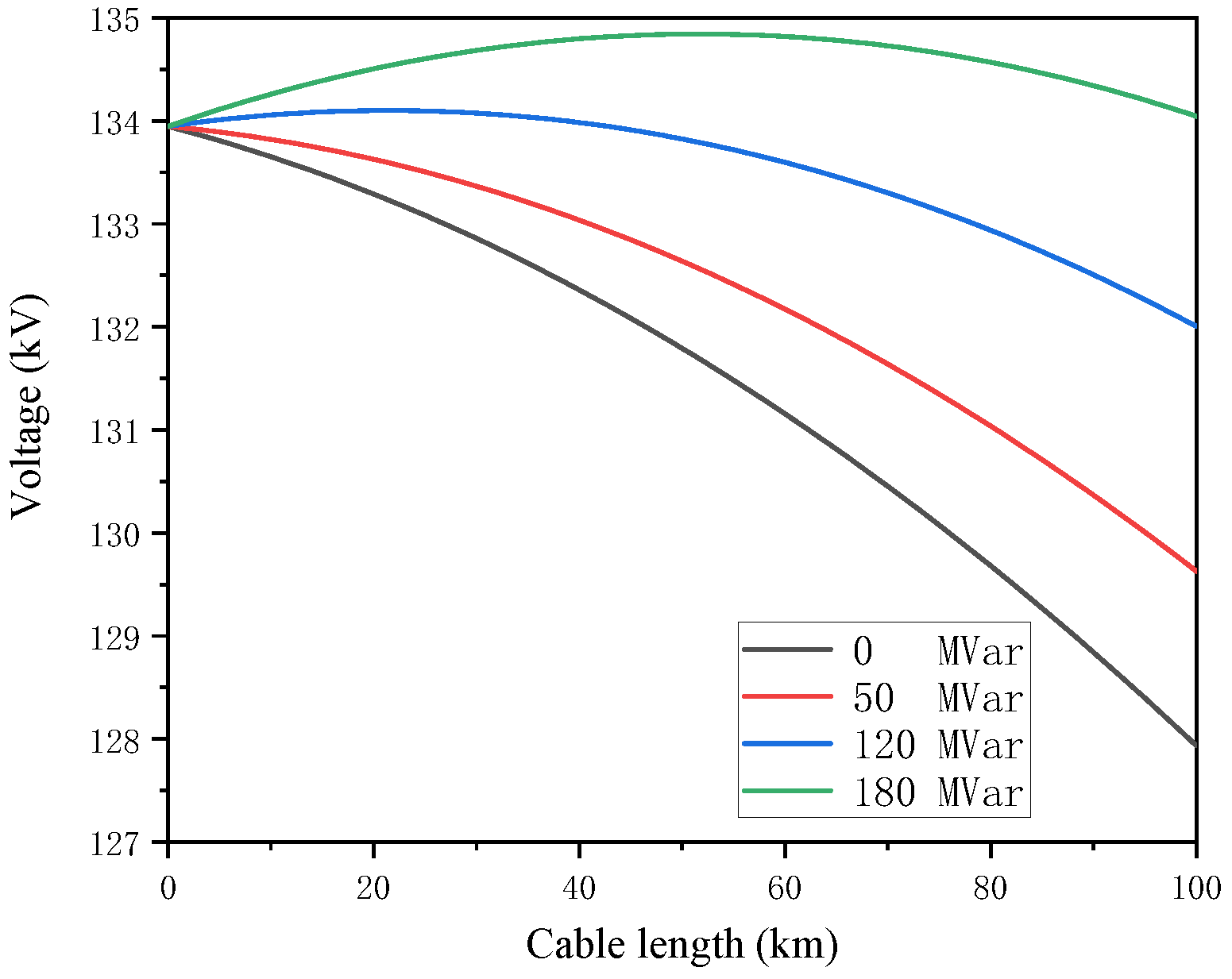
 Figure 7 and Figure 8, the current and voltage distribution curves of the submarine cable with different reactive power compensations at the sending end are obtained. According to Figure 7, the current at the sending end of the submarine cable line is related to the amount of reactive compensation. The larger the reactive power compensation at the sending end, the larger the current at the sending end. This is because the square of the current at the sending end is equal to the sum of the squares of the active current and reactive current. The relation between the current at the sending end of submarine cable line and the reactive compensation is as follows:
I 1 = P 3 V s cos θ 2 + Q s 3 V s 2
where P is the active power transmitted by the submarine cable line, W; QS is the reactive power compensated at the sending end of the line, Var.
On the other hand, the more reactive power compensated at sending end, the smaller the current at the receiving end is. This is because the inductive current of reactive power compensation at the sending end compensates part of the capacitive current of the line, making the reactive current of the line decrease. According to the U-shape current curve in Figure 7, in the case of sending end compensation, the maximum current of the whole line appears at the sending end or receiving end. In Figure 8, in the case of no compensation, the voltage on the line presents a downward trend, but applying reactive compensation at the sending end of the line will increase the voltage value on the line. When the reactive compensation reaches a certain degree, the voltage at the receiving end will exceed the voltage value at the sending end of the line. Applying a certain amount of reactive compensation to raise the voltage at the receiving end of the line can prevent the low voltage of the junction point and improve the stability of the system. The reactive power compensation for the receiving end does not change the current distribution of the line. According to the literature [30], the compensation for the receiving end can improve the power factor of the junction point.
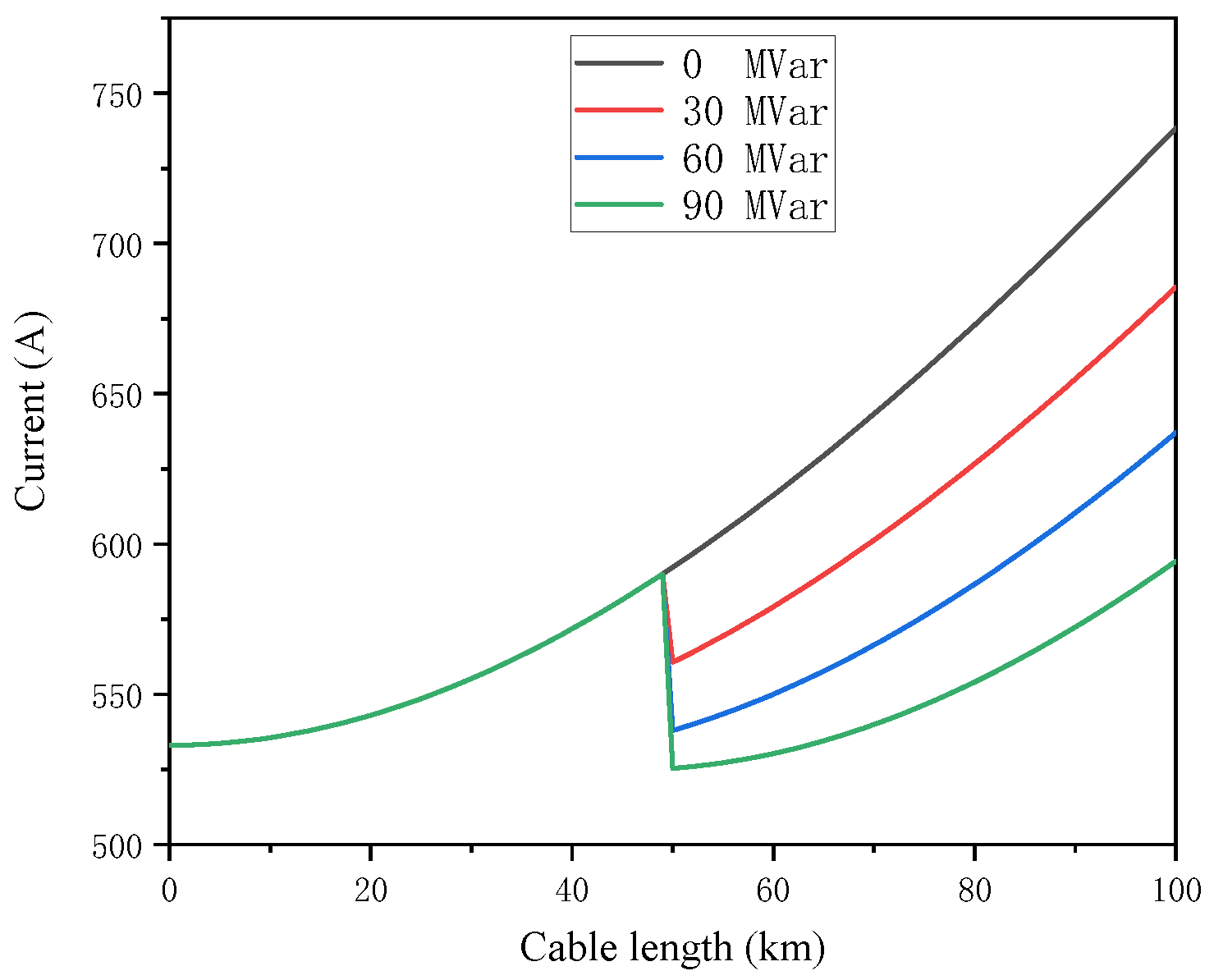
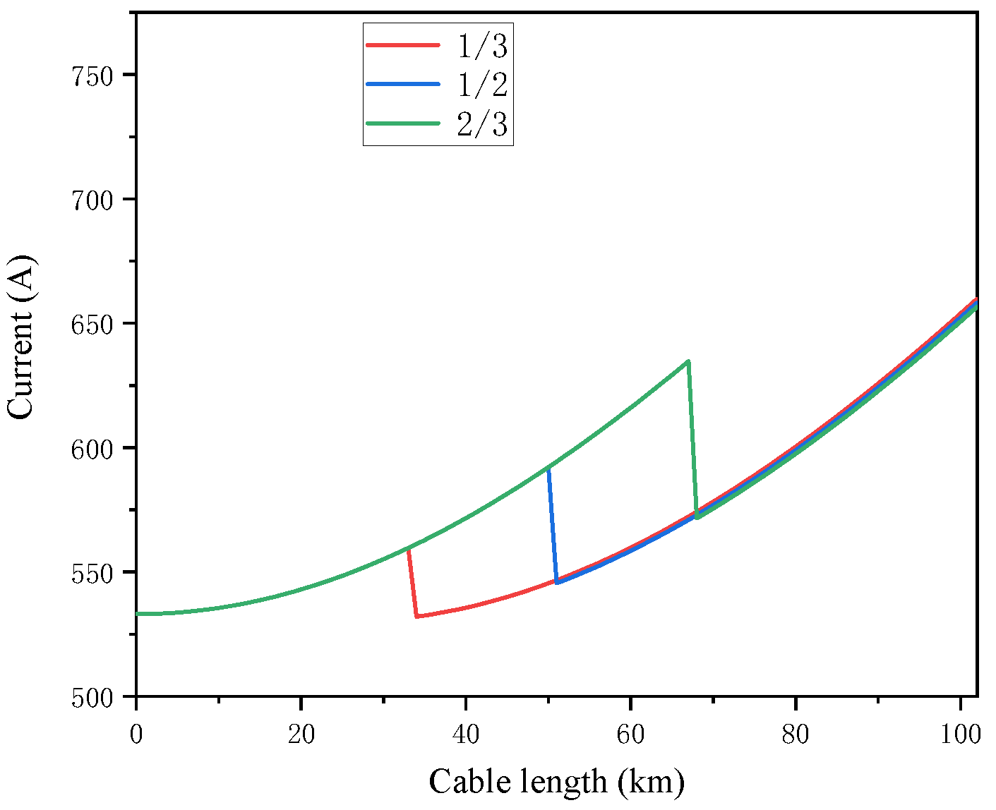
Middle line compensation refers to reactive power compensation on the submarine cable transmission line between the sending and receiving end. Compared with the compensation at the sending and receiving end, the reactive power compensation equipment are installed in the offshore booster station and the onshore centralized control center, respectively. Because submarine cables usually cross the sea, there are higher technical and economic requirements for the compensation at the middle line. For some submarine cable transmission lines crossing the island, the reactive power compensation can be considered in the island section. As shown in Figure 9, only the middle line of the submarine cable transmission line is compensated, and the current distribution from the sending end to the middle line does not change, while the reactive power compensation in the middle line will greatly reduce the current distribution from the middle section to receiving end. The current distribution results along the line after reactive power compensation at 1/3,1/2 and 2/3 of the long-distance submarine cable are calculated respectively, as shown in Figure 10. According to the Figure 10, the results show that the middle line compensation with the same capacity in different positions can reduce the current of the compensation point. But it will not change the current distribution trend from the compensation point to the receiving end.
To sum up, the receiving end compensation for submarine cable transmission lines will not change the current distribution on the lines, but it can be used as one of the measures to improve the power factor of junction points. The compensation for the mid-line can reduce the current distribution from the compensation point to the receiving end. However, the middle section of the submarine cable line is usually sea area, the cost for construction and maintenance of reactive compensation equipment for the mid-line is high. Therefore, to reduce the reactive current on the line and increase the transmission capacity of the line, the compensation for the sending end of the line is usually considered. The reactive compensation equipment is installed in offshore booster stations to reduce investment costs. For the long-distance transmission lines where sending end compensation cannot be satisfied, the mid-line compensation can be considered simultaneously.
The laying environment of submarine cable transmission line is complex, and the ampacity of different laying sections is different. If the current in a section of the line is greater than its ampacity, the cable core will overheat, accelerating the thermal aging of the insulation, and reducing the service life of the cable. Therefore, it is necessary to comprehensively consider the current distribution in the submarine cable lines and the ampacity of each section, and select the appropriate submarine cable laying mode and reactive power compensation scheme at the initial stage of the project design, it is better to realize the economy of investment.

4. Thermal Calculation Model of Submarine Cables

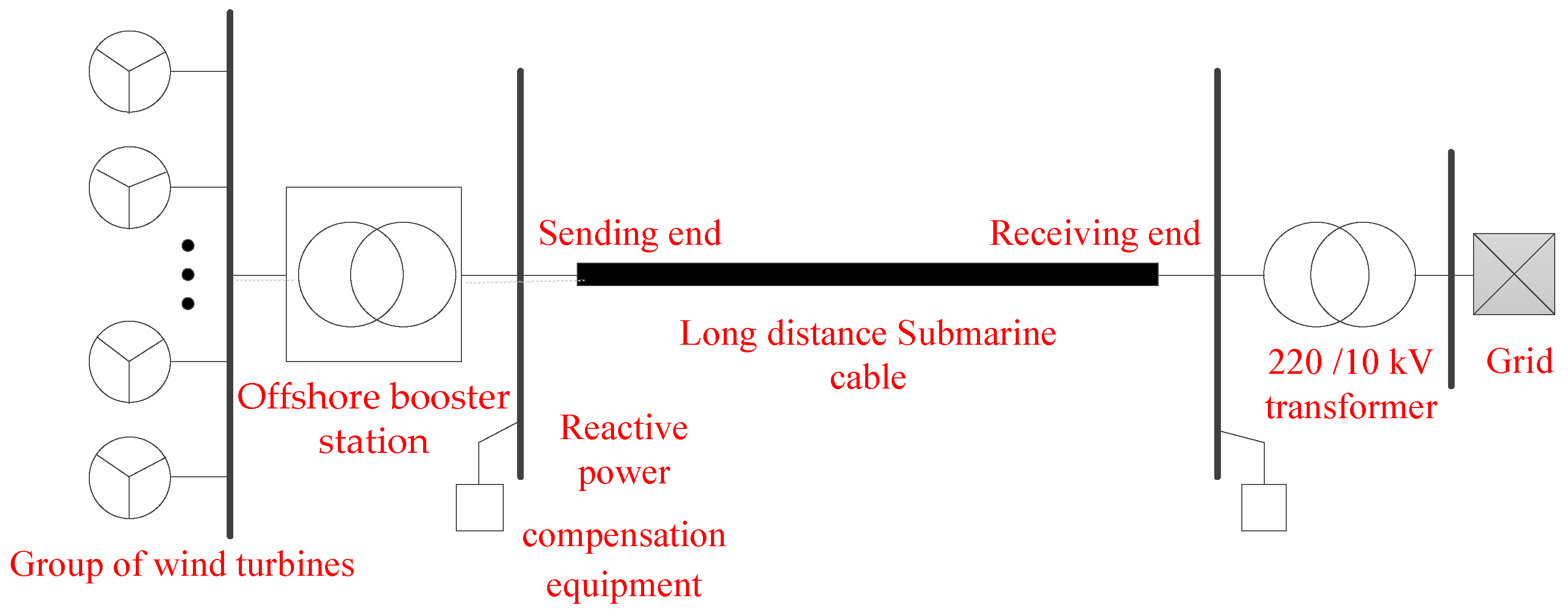
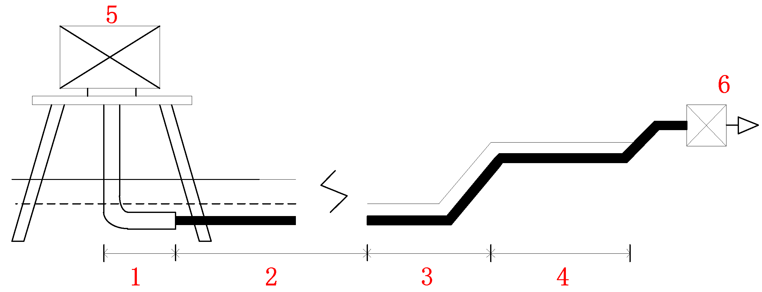
For the long-distance transmission lines of high-voltage output submarine cables in offshore wind farms, the starting point is usually the offshore booster station. The offshore booster station collects the electric energy generated by the wind turbine and boosts it, and then connects to the power grid on land through the submarine cables. It is generally composed of two parts: The power transformation system and the offshore platform structure. Then, the laying environment of the submarine cables is constantly changing, which can be mainly divided into four sections: J-shape pipe section, seabed section, mud flat section, and landing section. Finally, the line reaches the terminal station on land, and output cable laying path for offshore wind farm is shown in Figure 11. Generally, the J-shape pipe section gets the submarine cable to enter the sea from the offshore booster platform and lead to the seabed through the protection pipe [14]. In the seabed section, the cable is usually buried in the ground, and the buried depth is usually between 2 and 3 m. The length of the mud flat section is generally short, and it is the transition section between the seabed section and the landing section, directly buried laying is usually adopted. The landing section is generally buried in soil or laid in cable trench, and the length of this section is between several hundred meters and one or two kilometers. In this paper, it is assumed that the length of the J-shape pipe section is 30 m, the length of the mud flat section is 500 m, the length of the landing section is 2 km, and the rest of the length is the seabed section.
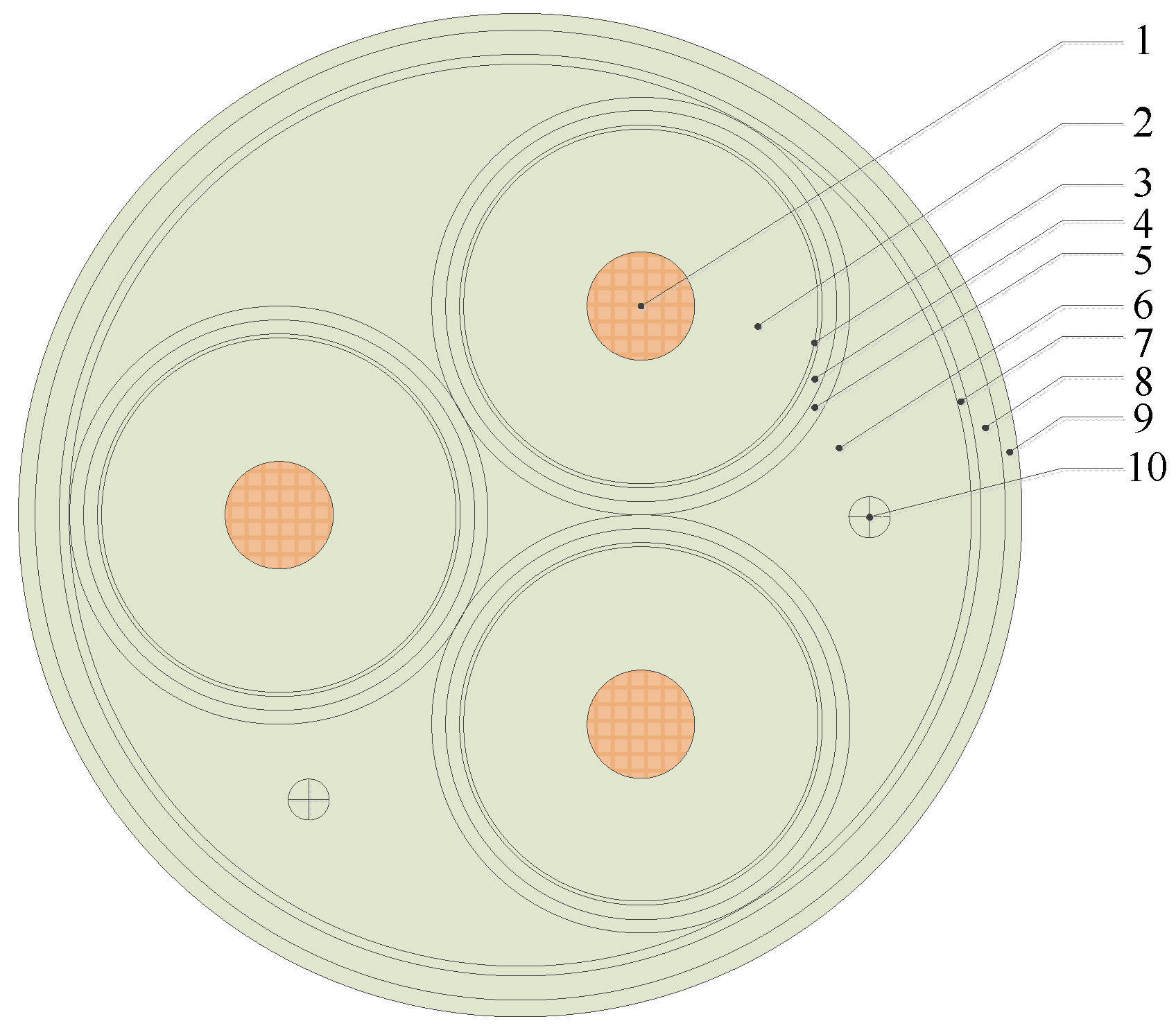
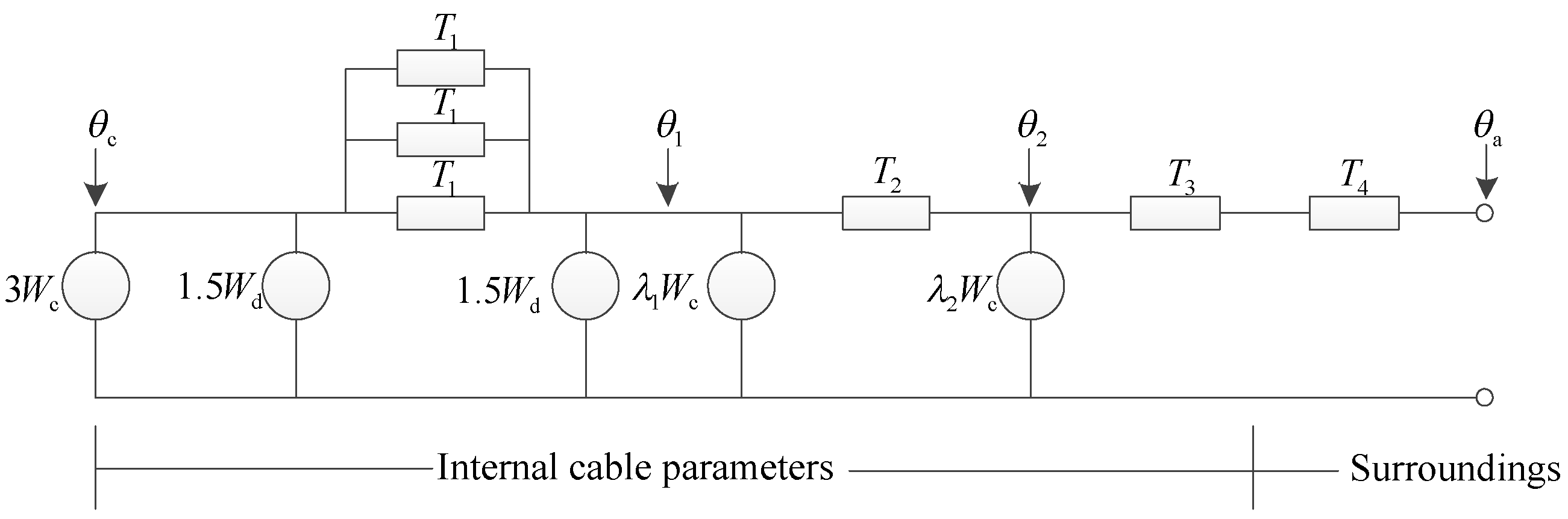
Based on the structural parameters of the three-core submarine cable, a thermal parameter model is established to calculate the ampacity of the submarine cable. The thermal parameters represent the heat flow through the materials of the cable. A steady-state thermal circuit model of a three-core submarine cable is as follows [32]:
In Figure 12, θc is the conductor temperature, θa is the environmental temperature of cable, θ1 is the metal sheath temperature, θ2 is the armor layer temperature, Wc is the joule loss of conductor per unit length, Wd is the dielectric loss of conductor insulation per unit length, T1 is the thermal resistance between conductor and sheath, T2 is the thermal resistance of the lining between sheath and armor, T3 is the thermal resistance of the outer sheath of the cable, and T4 refers to the thermal resistance between the cable surface and the surrounding medium. λ1 is the ratio of the metal sheath loss to the conductor loss, and λ2 is the ratio of the armor layer loss to the conductor loss.
The heat flow generated by the core loss of the submarine cable changes with the load. From the above thermal circuit model and the relation of thermoelectric analogy [32], according to the circuit node voltage method, the relation between temperature, heat flux, and thermal resistance of each part of the cable in steady state can be obtained:
3 W c + 1.5 W d T 1 3 = θ c θ 1
3 W c + W d + λ 1 W c T 2 = θ 1 θ 2
3 W c + W d + λ 1 W c + λ 2 W c T 3 + T 4 = θ 2 θ a
The allowable continuous ampacity of AC cable can be calculated according to the above equations and the empirical formula of ampacity calculation in IEC60287-1-1 [22], namely:
I = θ c θ a W d T 1 2 + n T 2 + T 3 + T 4 R T 1 + n R 1 + λ 1 T 2 + n R 1 + λ 1 + λ 2 T 3 + T 4 1 2
where, I is the allowable continuous current of the cable, A; n is the core number of submarine cable conductor, and R is the AC resistance of conductor under operating temperature. The calculation of relevant parameters can be found in Ref. [22].
R = R 1 + Y s + Y p
where, R′ is the DC resistance of conductor per unit length, Ω/m; Ys is the skin effect factor; and Yp is the adjacent effect factor.
λ 1 = λ 1 + λ 1
The metal sheath loss includes circulation loss λ1′ and eddy-current loss λ1″. The eddy-current loss is negligible for the three-core submarine cable. The calculation formula for the circulation loss λ1 is as follows.
λ 1 = R s R 1.5 1 + ( R s X ) 2
X = 2 ω 10 7 ln 2 s d
R s = ρ s A s 1 + α s θ η 20
where, S is the distance between conductor axes, m; d is the average diameter of the metal sheath, m; ρs is the conductivity of the metal sheath material, Ω·m; As is the cross-sectional area of the metal sheath, mm2; αs is the resistance temperature coefficient, 1/K; θ is the working temperature of conductor, °C; η is the ratio of the temperature of metal sheath to the temperature of conductor, were set as 0.7.
λ 2 = 1.23 R A R 2 c d A 2 1 2.77 R A 10 6 ω 2 + 1
where, RA is the AC resistance of armor layer at the highest temperature, Ω/m; c is the distance between the conductor axis and the center of submarine cable, m; dA is the average diameter of the armor layer, m.
W d = ω C U 0 tan δ
where, C is the submarine cable capacitance per unit length, F/m; U0 is the voltage to the ground, V; tanδ is the insulation loss factor under power frequency and working temperatures, here taken as t a n δ =   0.0005, w = 2 π f .
T 1 = K ρ T 2 π G
where, ρT is the thermal resistance coefficient of insulation, K·m/W; G is the geometric factor; and K is the shielding factor.
T 2 = ρ T 6 π G
where, G′ is the geometric factor; and ρT is the thermal resistance coefficient between sheath and armor, K·m/W.
T 3 = 1 2 π ρ T ln 1 + 2 t 3 D a
where, ρT is the thermal resistance coefficient of submarine cable outer sheath, K·m/W; t3 is the thickness of outer sheath, m; Da is the outer diameter of the armor, m; and the calculation formula for the environmental thermal resistance T4 depends on the laying environment, as shown below:
T 4 = ρ T 2 π I n 4 L D e 1 π D e h Δ θ tr 0.25 T 4 a + T 4 b + T 4 c = U 1 + 0.1 V + Y θ m D e + ρ d 2 π I n D o D d + 1 π D o h Δ θ 0.25
Equation (24) correspond to the calculation formulas of environmental thermal resistance under the laying methods of directly buried, cable trench, and J-shape pipe laying, respectively. Where, ρT is the thermal resistance coefficient of soil, K·m/W; L is the buried depth of submarine cables, m, which is the distance between the cable axis and the ground surface; De is the outside diameter of the cable, m; h is the coefficient of heat transfer on the cable surface, W/m2·K; Δθtr is the temperature rise when the air temperature in the cable trench is higher than the surrounding air temperature, K; T4a, T4b, and T4c are, respectively, the air thermal resistance, the J-shape pipe thermal resistance, and the pipe external thermal resistance, which are between the cable surface and the inner surface of the pipe; U, V, and Y are constants related to laying conditions; θm is the average temperature of medium between cables and pipelines, K; Do is the outer diameter of the pipe, m; Dd is the pipe inner diameter, m; ρd is the thermal resistance of J-shape pipe material, K·m/W; hj is the coefficient of heat transfer on the surface of the J-shape pipe, W/m2 ·K; Δθ is the temperature rise when the temperature of J-shape pipe is higher than the surrounding air temperature, K.
For the four laying methods of output cables in offshore wind farms (J-shape pipe section, seabed section, mud flat section, and landing section), the parameter assumptions of different laying environments are given for the ampacity calculation, and the ampacity of different sections are calculated. The relevant parameters and calculation results are shown in Table 3 and Table 4, respectively.

5. Reactive Power Compensation Analysis of Submarine Cables Based on Electrothermal Coordination

Due to the limitation of thermal stability, the submarine cable should meet the requirement that the current of the whole line should not be greater than its ampacity. Meanwhile, the operation principle of the high-voltage AC transmission system should also be considered. To maintain the stability of the system, the voltage excursion of sending and receiving end sections of the transmission line should be contained within a suitable range, and the power factors of offshore booster stations and onshore junction points also need to meet a certain range. The current distribution of long-distance submarine cable transmission line needs to meet the requirement of ampacity of each section under different laying modes. The relevant constraint conditions are shown as follows [10,30].
cos φ 1 0.95
cos φ 2 = 1
0.97 V n V s 1.07 V n
0.97 V n V r 1.07 V n
I line I rated
where, cosφ1 and cosφ2 are the transmission power factors of the sending and receiving end of the submarine cable line, respectively; Vn is the rated voltage of the line at 220 kV; Iline is the current value in the submarine cable transmission line, A; Irated is the ampacity of each section of the line under different laying methods, A.
For the long-distance submarine cable transmission lines, by considering the above constraints, the current distribution of different reactive power compensation schemes is analyzed. The more economical compensation schemes and landing section laying methods are selected, to realize the economic and safe operation of the submarine cable. The offshore wind farms transmit the maximum current at its full load. Being affected by charging current, the current of the line at full load may exceed its ampacity, so the full load condition is considered in the analysis below.

5.1. Directly Buried Laying Method of Landing Section

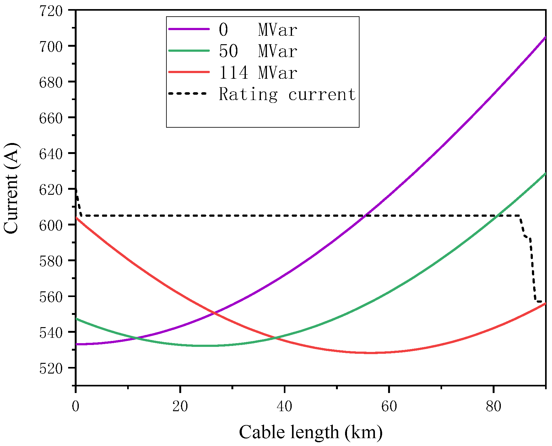
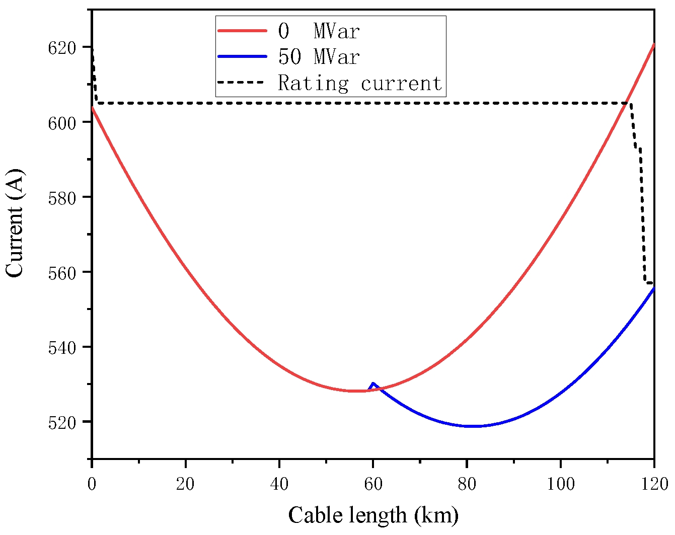
First, the directly buried laying method is considered in the landing section. The ampacity of the directly buried laying method in the landing section, which is calculated from Table 4, is 557 A. After calculation, for the submarine cable transmission lines with a length of 90 km or less, the ampacity will meet the requirement through conducting the reactive power compensation at sending end. The results calculated by MATLAB are shown in Figure 13.
As shown in the figure above, the dotted line represents the ampacity of different laying sections of long-distance submarine cables. The bottleneck point of submarine cables ampacity occurs in the landing section. When there is no reactive compensation, the current at the end of the transmission line is far greater than its ampacity due to the large charging current, and it causes the core conductor temperature to exceed 90 °C, accelerating insulation aging. After reactive compensation, the current distribution on the transmission line changes obviously. When the reactive power compensation amount at the sending end is 50 MVar, the current at the receiving end of the line is still greater than the ampacity of this section. When the compensation at sending end reaches 114 MVar, the current at receiving end of the line decreases, while the current at sending end of the line increases. The current distribution in the line does not exceed the ampacity of each section.
For the submarine cable transmission lines with a transmission distance greater than 90 km, the directly buried laying method is adopted in the landing section. Only conducting reactive compensation at the sending end of the line cannot meet the requirement of ampacity. As a result, conducting the reactive compensation at mid-line of the transmission line is considered. The reactive power compensations are conducted at the sending and receiving ends and the mid-line at the same time, and the calculation results are shown in Figure 14.
According to Figure 14, when the submarine cable transmission line is 120 km in length, and the reactive power compensation is only carried out at the sending end of line, the current at the receiving end of the line is still far greater than its ampacity. Choose to conduct compensation of 114 MVar and 50 MVar at the sending end and mid-line respectively, and the reactive compensation for receiving end is applied to meet the requirement of power factor. As shown in the figure above, conducting reactive power compensation at mid-line can significantly reduce the current at receiving end, but it does not change the current distribution from sending end to mid-line. It can be considered as a reactive compensation solution for the long-distance submarine cable transmission lines if there are sea islands in the middle section path of lines.

5.2. Cable Trench Laying Method in Landing Section
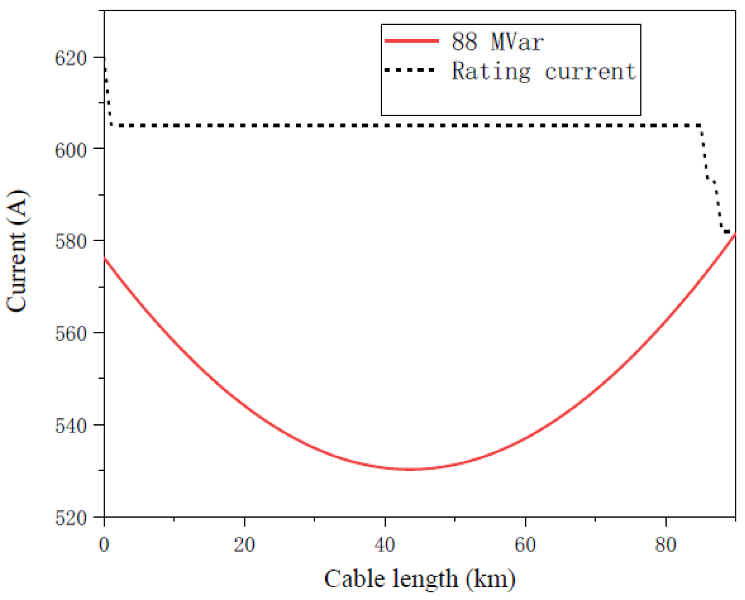
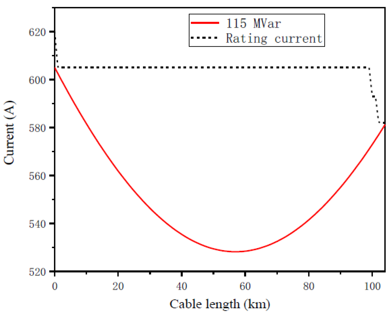
As shown in Figure 15, the cable trench laying method is adopted in the landing section of the submarine cable transmission lines with a transmission distance of 90 km. Compared with the directly buried laying method, due to the better heat dissipation conditions in the cable trench and smaller environmental thermal resistance, the calculated ampacity is larger. The ampacity of landing section with cable trench laying method is 582 A. When the sending end reactive compensation capacity reaches 88 MVar, the current in the line can meet the requirement of ampacity. In Figure 16, the maximum transmission distance of the submarine cable transmission line is 104 km when adopting the cable trench laying mode in the landing section, and the reactive power compensation at sending end is 115 MVar, which can meet the requirement of ampacity.

6. Conclusions

This study considers a long-distance high voltage AC three-core submarine cable from a real offshore wind farm project. An accurate cable model is used to analyze the influence of reactive power compensation in different positions on the current distribution on the line, and optimizing the existing reactive power compensation schemes based on ETC. From the analysis, the following conclusions are obtained:
(1)
When the long-distance submarine cable is compensated for reactive power, not only the stability of the system should be maintained, but also the thermal limits of the submarine cable should be considered. The bottleneck of offshore wind farm output submarine cable ampacity appears in the landing section.
(2)
Conducting reactive compensation at sending end of the line can reduce the current at the receiving end. On the contrary, it can raise the current at the sending end of the line. The maximum current occurs at the sending or receiving end of the line depending on the capacity of reactive power compensation.
(3)
According to ETC, the current of long-distance submarine cable should be less than the ampacity under the condition of reactive power compensation. The cable trench laying method can improve the cable ampacity of landing section and thus reduce the capacity of reactive power compensation at sending end.

Author Contributions

Conceptualization, G.L., M.F., and P.W.; methodology, G.L.; software, M.F. and P.W.; validation, G.L., M.F., and P.W.; formal analysis, M.F. and P.W.; investigation, all authors.; resources, M.Z.; data curation, M.Z.; writing—original draft preparation, G.L. and M.F.; writing—review and editing, M.F. and P.W.; visualization, M.F. and M.Z.; supervision, G.L. and P.W.; project administration, M.Z.; funding acquisition, G.L. All authors have read and agreed to the published version of the manuscript.

Funding

This work is the output of the research project “Life cycle cost analysis and evaluation of submarine power cables”[EX02061W], supported by Guangdong Electric Power Design Institute of Chinese Energy Engineering Group in Guangzhou.

Institutional Review Board Statement

Not applicable.

Informed Consent Statement

Not applicable.

Data Availability Statement

Not applicable.

Conflicts of Interest

The authors declare no conflict of interest.

References

  1. Soares-Ramos, E.P.; De Oliveira-Assis, L.; Sarrias-Mena, R.; Fernández-Ramírez, L.M. Current status and future trends of offshore wind power in Europe. Energy 2020, 202, 117787. [Google Scholar] [CrossRef]
  2. GWEC. Global Wind Report; GWEC: Belgium, Brussels, 2019. [Google Scholar]
  3. Schifreen, C.S.; Marble, W.C. Charging Current Limitations in Operation or High-Voltage Cable Lines [includes discussion]. Trans. Am. Inst. Electr. Eng. Part III Power Appar. Syst. 1956, 75, 803–817. [Google Scholar] [CrossRef]
  4. Todorovic, J. Losses Evaluation of HVAC Connection of Large Offshore Wind Farms. Master’s Thesis, Royal Institute of Technology, Stockholm, Sweden, December 2004. [Google Scholar]
  5. Alassi, A.; Santiago, B.; Omar, E.; Grain, A.; Callum, M. HVDC transmission: Technology review, market trends and future outlook. Renew Sustain. Energy Rev. 2019, 112, 530–535. [Google Scholar] [CrossRef]
  6. Gustavsen, B.; Mo, O. Variable Transmission Voltage for Loss Minimization in Long Offshore Wind Farm AC Export Cables. IEEE Trans. Power Deliv. 2016, 32, 1422–1431. [Google Scholar] [CrossRef] [Green Version]
  7. Ruddy, J.; Meere, R.; O’Donnell, T.; Jonathan, R. Low Frequency AC transmission as an alternative to VSC-HVDC for grid interconnection of offshore wind. In 2015 IEEE Eindhoven PowerTech; IEEE: New York, NY, USA, 2015; pp. 1–6. [Google Scholar]
  8. Gatta, F.; Geri, A.; Lauria, S.; Maccioni, M. Steady-state operating conditions of very long EHVAC cable lines. Electr. Power Syst. Res. 2011, 81, 1525–1533. [Google Scholar] [CrossRef]
  9. Perdana, A.; Carlson, O. Factors Influencing Design of Dynamic Reactive Power Compensation for an Offshore Wind Farm. Wind Eng. 2009, 33, 273–285. [Google Scholar] [CrossRef]
  10. Dicorato, M.; Forte, G.; Trovato, M.; De Tuglie, E. Control strategy for regulating reactive power exchange in offshore wind farm. In Proceedings of the 2010 IEEE International Symposium on Industrial Electronics, Bari, Italy, 4–7 July 2010; pp. 2363–2370. [Google Scholar] [CrossRef]
  11. Wind Turbines Connected to Grids with Voltages above 100 kV—Technical Regulation for the Properties and the Regulation of Wind Turbines. In Energinet Technical Regulation 3.2.5; Elkraft Systems and Eltra: Fredericia, Denmark, 3 December 2004.
  12. The Grid Code Connection Conditions; National Grid: London, UK, 2009.
  13. Pilgrim, J.A.; Catmull, S.; Chippendale, R.D.; Lewin, P.L.; Stratford, P.; Tyreman, R. Current rating optimisation for offshore wind farm export cables. In Proceedings of the Cigre Session 2014, Paris, France, 24–29 August 2014. [Google Scholar]
  14. Chippendale, R.D.; Pilgrim, J.A.; Goddard, K.F.; Cangy, P. Analytical Thermal Rating Method for Cables Installed in J-Tubes. IEEE Trans. Power Deliv. 2017, 32, 1721–1729. [Google Scholar] [CrossRef] [Green Version]
  15. You, L.; Wang, J.; Liu, G.; Ma, H.; Zheng, M. Thermal Rating of Offshore Wind Farm Cables Installed in Ventilated J-Tubes. Energies 2018, 11, 545. [Google Scholar] [CrossRef] [Green Version]
  16. Wang, P.-Y.; Ma, H.; Liu, G.; Han, Z.-Z.; Guo, D.-M.; Xu, T.; Kang, L.-Y. Dynamic Thermal Analysis of High-Voltage Power Cable Insulation for Cable Dynamic Thermal Rating. IEEE Access 2019, 7, 56095–56106. [Google Scholar] [CrossRef]
  17. Hughes, T.J.; Henstock, T.J.; Pilgrim, J.A.; Dix, J.K.; Gernon, T.M.; Thompson, C.E.L. Effect of Sediment Properties on the Thermal Performance of Submarine HV Cables. IEEE Trans. Power Deliv. 2015, 30, 2443–2450. [Google Scholar] [CrossRef]
  18. Bonnard, C.-H.; Blavette, A.; Bourguet, S.; Charmetant, A. Modeling of a wave farm export cable for electro-thermal sizing studies. Renew. Energy 2020, 147, 2387–2398. [Google Scholar] [CrossRef]
  19. Kolluri, S.; Thummala, P.; Sapkota, R.; Panda, S.K.; Rendusara, D. Subsea power transmission cable modelling: Reactive power compensation and transient response studies. In Proceedings of the 2016 IEEE 17th Workshop on Control and Modeling for Power Electronics (COMPEL), Trondheim, Norway, 27–30 June 2016; pp. 1–6. [Google Scholar] [CrossRef]
  20. Benato, R.; Paolucci, A. Operating capability of long AC EHV transmission cables. Electr. Power Syst. Res. 2005, 75, 17–27. [Google Scholar] [CrossRef]
  21. Xie, Y.; Zhao, Y.; Bao, S.; Wang, P.; Huang, J.; Liu, G.; Hao, Y.-P.; Li, L. Investigation on Cable Rejuvenation by Simulating Cable Operation. IEEE Access 2020, 8, 6295–6303. [Google Scholar] [CrossRef]
  22. IEC 60287-1-1:2006. Electric Cables—Calculation of the Current Rating—Part 1-1: Current Rating Equations (100 % Load Factor) and Calculation of Losses—General; International Electrotechnical Commission: Geneva, Switzerland, 2006; Available online: https://webstore.iec.ch/publication/1265 (accessed on 15 January 2021).
  23. Olsen, R.S.; Holboell, J.; Gudmundsdottir, U.S. Electrothermal Coordination in Cable Based Transmission Grids. IEEE Trans. Power Syst. 2013, 28, 4867–4874. [Google Scholar] [CrossRef]
  24. Banakar, H.; Alguacil, N.; Galiana, F. Electrothermal Coordination Part I: Theory and Implementation Schemes. IEEE Trans. Power Syst. 2005, 20, 798–805. [Google Scholar] [CrossRef]
  25. Huang, Q.; Wang, X.; Fan, J.; Zhang, X.; Wang, Y. Reliability and economy assessment of offshore wind farms. J. Eng. 2019, 2019, 1554–1559. [Google Scholar] [CrossRef]
  26. GB/T 19963-2011. Technical Rule for Connecting Wind Farm to Power System, National Electric Power Regulatory Standardization Technical Committee; China Standards Press: Beijing, China, 2011; Available online: http://www.gb688.cn/bzgk/gb/newGbInfo?hcno=C0B59C55FD4B287CDF02842D074D1476 (accessed on 15 January 2021).
  27. Gatta, F.; Geri, A.; Lauria, S.; Maccioni, M. Steady-state operating conditions of very long EHVAC cable lines: Two case studies. Electr. Power Syst. Res. 2012, 83, 160–169. [Google Scholar] [CrossRef]
  28. Benato, R.; Sessa, S.D.; Forzan, M.; Marelli, M.; Pietribiasi, D. Core laying pitch-long 3D finite element model of an AC three-core armoured submarine cable with a length of 3 metres. Electr. Power Syst. Res. 2017, 150, 137–143. [Google Scholar] [CrossRef]
  29. Carson, J.R. Wave Propagation in Overhead Wires with Ground Return. Bell Syst. Tech. J. 1926, 5, 539–554. [Google Scholar] [CrossRef]
  30. Guiping, Z.; Xiaowei, D.; Chen, Z. Optimisation of reactive power compensation of HVAC cable in off-shore wind power plant. IET Renew. Power Gener. 2015, 9, 857–863. [Google Scholar] [CrossRef]
  31. Song-Manguelle, J.; Todorovic, M.H.; Chi, S.; Gunturi, S.K.; Datta, R. Power Transfer Capability of HVAC Cables for Subsea Transmission and Distribution Systems. IEEE Trans. Ind. Appl. 2014, 50, 2382–2391. [Google Scholar] [CrossRef]
  32. Nielsen, T.V.M.; Jakobsen, S.; Savaghebi, M. Dynamic Rating of Three-Core XLPE Submarine Cables for Offshore Wind Farms. Appl. Sci. 2019, 9, 800. [Google Scholar] [CrossRef] [Green Version]
Figure 1. Model diagram of an offshore wind farm connected to a power grid.
Jmse 09 00090 g001
Figure 2. Simplified cross section of three-core submarine cable. 1–core conductor; 2–cross-linked polyethene (XLPE) insulation layer; 3–swelling tape; 4–metal sheath; 5–PE sheath; 6–filling layer and wrapping tape; 7–inner sheath; 8–armor layer; 9–outer serving; 10–fiber layer [28].
Jmse 09 00090 g002
Figure 3. PI equivalent model of transmission lines.
Jmse 09 00090 g003
Figure 4. Segmentation of submarine cable into n sections for assessment of internal currents and voltages.
Jmse 09 00090 g004
Figure 5. Submarine cable lines with n sections of PI equivalent circuits.
Jmse 09 00090 g005
Figure 6. Current distribution of submarine cables under different load conditions without reactive power compensation.
Jmse 09 00090 g006
Figure 7. Current distribution of submarine cables under full load with different reactive power compensation at the sending end.
Jmse 09 00090 g007
Figure 8. Voltage distribution of submarine cables under full load with different reactive power compensation at the sending end.
Jmse 09 00090 g008
Figure 9. Current distribution of submarine cables under full load with different reactive power compensation at the middle line.
Jmse 09 00090 g009
Figure 10. Current distribution of long-distance submarine cables under reactive power compensation at different positions.
Jmse 09 00090 g010
Figure 11. Output cable laying path for offshore wind farm. 1—J-shape pipe section; 2–seabed section; 3–mud flat section; 4–landing section; 5–offshore booster station platform; 6–onshore centralized control center.
Jmse 09 00090 g011
Figure 12. Steady-state thermal circuit model of three-core submarine cable.
Jmse 09 00090 g012
Figure 13. Comparison of current distribution of submarine cables under reactive power compensation at the sending end with the full-line ampacity under directly buried laying in landing section.
Jmse 09 00090 g013
Figure 14. Comparison of current distribution of submarine cables under reactive power compensation at mid-line with the full-line ampacity under directly buried laying in landing section.
Jmse 09 00090 g014
Figure 15. Comparison of current distribution of 90 km submarine cables under reactive power compensation at the sending end with the full-line ampacity under trench laying in the landing section.
Jmse 09 00090 g015
Figure 16. Comparison of current distribution of 104 km submarine cables under reactive power compensation at the sending end with the full-line ampacity under trench laying in the landing section.
Jmse 09 00090 g016
Table 1. Structural parameters of submarine cables.
Layer
Number
StructureThickness/mmOuter Radius of Structure/mm
1Core conductor13.3
2XLPE insulation27.043.7
3Swelling tape0.544.7
4Metal sheath3.548.2
5PE sheath3.351.5
6Filling layer0.6112.15
7Inner sheath1113.65
8Armored layer6.0119.65
9Outer serving4.0123.65
Table 2. Distribution parameters of three-core AC submarine cable.
ParametersResistance
Ω/km
Inductance
mH/km
Conductance
S/km
Capacitance
µF/km
Value0.04880.432.11 × 10−80.1283
Table 3. Parameters of submarine cable laying conditions.
Material ParametersValue
Thermal conductivity coefficient of soil at landing section (K·m/W)1.2
Thermal conductivity coefficient of soil at mud flat section (K·m/W)1
Thermal conductivity coefficient of soil at seabed section (K·m/W)0.83
J-shape pipe inner diameter (mm)468
J-shape pipe outer diameter (mm)508
Table 4. Submarine cable laying conditions and ampacity.
Laying EnvironmentEnvironment Temperature °CLaying Depth mThermal Resistance T4Ampacity A
J-shape pipe section55-0.16620
Seabed section28.52.50.49605
Mud flat section3510.443593
Landing section (directly buried)3510.532557
Landing section (cable trench)5010.2766582
Publisher’s Note: MDPI stays neutral with regard to jurisdictional claims in published maps and institutional affiliations.

