
A Model-Derived Empirical Formulation for Wave Run-Up on Naturally Sloping Beaches


1
Deltares, Marine and Coastal Systems, Boussinesqweg 1, 2629 HV Delft, The Netherlands
2
IHE Delft Institute for Water Education, Coastal and Urban Risk and Resilience, 2601 DA Delft, The Netherlands
*
Author to whom correspondence should be addressed.
J. Mar. Sci. Eng. 2021, 9(11), 1185; https://0-doi-org.brum.beds.ac.uk/10.3390/jmse9111185
Submission received: 1 September 2021
/
Revised: 13 October 2021
/
Accepted: 18 October 2021
/
Published: 27 October 2021
(This article belongs to the Topic From Coastal Engineering to Integrated Coastal Zone Management)
Abstract
:A new set of empirical formulations has been derived to predict wave run-up at naturally sloping sandy beaches. They are obtained by fitting the results of hundreds of XBeach-NH+ model simulations. The simulations are carried out over a wide range of offshore wave conditions (wave heights ranging from 1 to 12 m and periods from 6 to 16 s), and surf zone (Dean parameters aD ranging from 0.05 to 0.30) and beach geometries (slopes ranging from 1:100 to 1:5). The empirical formulations provide estimates of wave set-up, incident and infragravity wave run-up, and total run-up R2%. Reduction coefficients are included to account for the effects of incident wave angle and directional spreading. The formulations have been validated against the Stockdon dataset and show better skill at predicting R2% run-up than the widely used Stockdon relationships. Unlike most existing run-up predictors, the relations presented here include the effect of the surf zone slope, which is shown to be an important parameter for predicting wave run-up. Additionally, this study shows a clear relationship between infragravity run-up and beach slope, unlike most existing predictors.
1. Introduction
Coastal zones are subject to wave and wind-induced hazards such as wave attack, flooding, and erosion. Worldwide, these coastal hazards affect millions of people living in low-lying coastal zones. With sea level rise and potentially an increase in storm and cyclone activity, this will increase substantially over the coming century.
It is therefore important to be able to reliably assess (in planning studies) and to forecast (in operational systems) the Total Water Levels (TWL) caused by wind- and wave-processes. Wind fields associated with storms exert a shear stress on the water surface which causes a water level gradient towards the coast called storm surge. This is exacerbated by the inverse barometer effect which causes an uplift of the water surface by the low-pressure fields near the eye of the storm. These wind-induced processes have been incorporated into hydrodynamic forecast and planning models such as Delft3D [1], ADCIRC [2], and SLOSH [3], which are routinely used.
The wave-driven component of the TWL consists of a mean set-up and swash run-up. The mean set-up is caused by wave breaking which exerts a wave-stress (the radiation stress [4]), which is balanced by a gradient in the water level towards the shore. The swash is the oscillatory motion of waves in the infragravity (0.004–0.04 Hz) and incident or sea-swell band (0.04–0.5 Hz) that run up and down the beach. The sum of tides, surge, mean set-up, and the crests of the oscillatory run-up motion are called the TWL. The wave contribution to the TWL may be in the order of 20% [5] on mildly sloping coasts and may be dominant on steeper coasts [6]. While the processes are largely understood and incorporated in numerical models which show considerable skill (e.g., [6,7]), process-based models to compute run-up are not routinely incorporated in forecast systems because of their computational expense. Rather, run-up formulas which are based on field observations (e.g., the Stockdon formula [8]) are typically applied [9]. The Stockdon formula [8] is the most widely used, but it is a class of empirical formulas which includes those in [10,11,12,13], among many others. A very thorough overview of existing run-up predictors and their performance is provided by Gomes da Silva [13].
While these formulas have been derived based on most of the available field observations, the overall set of observations is still small, which limits the applicability beyond the observed conditions (which have been mild mostly) and geomorphological setting (which have mostly been sandy shorelines). However, in absence of better widely applicable formulations, the empirical formulas are routinely used, which may result in an under- or overestimation of run-up levels in more extreme conditions. Both these deviations are undesired: they may result in false positives or negatives in forecasts, and in over- or under-dimensioning of coastal protection structures.
One way to extend the validity of the formulations is to actively observe run-up on a wider variety of coasts (e.g., on coral-reef lined coasts [14]) and to rapidly respond with quickly deployable field equipment to observe more extreme events, but this is costly and will increase the validity of new models only slowly in time. Physical laboratory tests of run-up can also be used to train empirical relations, although these may suffer from scaling effects. Another approach is to use numerical models in prototype scale to provide data on the basis of which more generalized formulas, or meta-models, can be derived. Stockdon [15] attempted to extend the validity of the empirical formula under more extreme conditions using the surfbeat version of XBeach [16,17], which is not capable of resolving incident swash motions. Furthermore, they found a relatively strong underestimation of modelled infragravity motions in 2D simulations.
In the present approach study, we apply the XBeach-NH+ model [18] which is a quasi-two-layer dispersive model which resolves both the incident and infragravity waves up to a relative depth kh of 4. This model has shown good skill in predicting the wave hydrodynamics in field conditions [6] and wave run-up in laboratory conditions [7]. This model, using calibrated settings, is applied to a wide range of geomorphological parameters/coastal types and for a wide range of wave forcing conditions, including obliquely incident waves and wave directional spreading. The computed run-up levels are treated as observed data and are used to fit a new empirical “VO21” formulation for the individual set-up zmean, infragravity run-up SIG, incident run-up Sinc, and total run-up R2% components. Furthermore, reduction coefficients are derived to account for the effects of incident wave angle and directional spreading, using the results of a limited set of 2D XBeach-NH+ simulations.
The new formulations are validated against the Stockdon dataset [8]. The main aim of this study is not to explain the physics behind the derived relationships, but rather to define a set of empirical relations that can be used in engineering and forecasting applications. The implications for future use, the limitations of applicability, and next steps are discussed.
2. Methods
The empirical relations presented in this paper were derived from many 1D XBeach-NH+ model runs [18], in which a wide range of offshore boundary conditions and cross-shore geometries were simulated. Time series of vertical run-up were extracted from the results, and from these the mean set-up (zmean), and the incident (Sinc) and infragravity (SIG) components were computed. Next, empirical relations were defined that describe zmean, Sinc, and SIG as a function of the offshore wave height, and dimensionless surf zone and beach Irribarren numbers [19]. A relationship was then found that describes the R2% run-up as a function of zmean, Sinc, and SIG. Finally, a set of reduction factors was derived to account for the effects of incident wave direction and directional spreading from a limited set of 2D simulations. The synthetic model data have not been divided here into training and testing data. The entire synthetic dataset was used for training. The Stockdon field dataset [8] was used for testing.
2.1. Model Set-Up
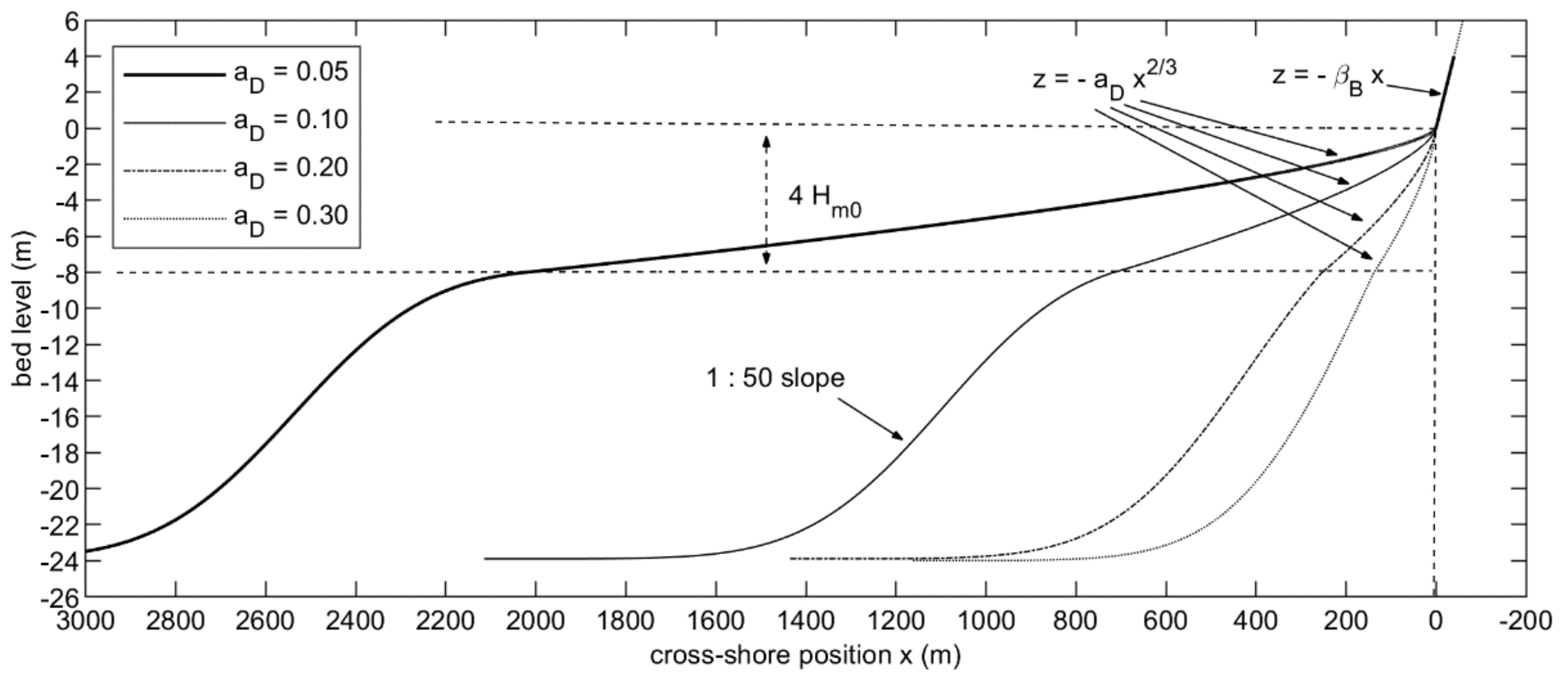
For the new empirical relations to be valid over a wide range of conditions, we chose a large set of offshore wave conditions (ranging from long-distance swell to locally generated storm waves) and morphologic parameters (from very mild to very steep sloping beaches). Each of the runs was carried out with varying offshore wave height (Hm0) and period (Tp), surf zone steepness (Dean parameter aD [20]) and beach slope (tan βb) (see Table 1), resulting in an initial set of 5 × 4 × 4 × 5 = 400 model runs. Unlikely (but not impossible) combinations with either very mild foreshores and very steep beaches or very steep foreshores and very mild-sloping beaches were also included in the set of simulations. Conditions, however, with physically unrealistic values for deep-water wave steepness (>0.04) were removed (e.g., Hm0 = 16 m and Tp = 6 s). This results in a final set of 280 simulations.
An example of a cross-shore profile is given in Figure 1. At the dry beach, the profile has a slope of tan βb. The profile in the surf zone is schematized with a Dean profile [20] up to a depth of 4 times the offshore wave height. Beyond the surf zone, the bathymetry gradually drops to a depth where n (C/Cg) equals 0.8 [18]. The cross-shore grid resolution varies along the profile, such that individual waves are covered by approximately 80 grid cells. The minimum and maximum cross-shore grid spacing were set to 0.2 m and 5.0 m, respectively.
All model simulations were carried out for a 3 h period during which the offshore boundary conditions were kept constant. Deep-water waves (from Table 1) were first shoaled to the depth of the model boundary. At the boundary, the incoming waves were generated by XBeach-NH+ assuming a JONSWAP spectrum with a peak enhancement factor of 3.3.
A constant Chezy roughness (C = 70) was applied. Vertical run-up time series zt were obtained from a run-up gauge in the model which tracks the most landward wet point. The threshold water depth for determining whether a grid cell is wet was set to 0.01 m. Tests with this parameter did not show strong sensitivity to the results in the range between 0.01 and 0.05 m. The maximum breaker steepness was set to 0.6, as recommended by [18].
In addition to the 1D profile simulations, a limited number of 2D runs were carried out to investigate the effects of the incident wave angle and directional spreading, as, by definition, the 1D profile models cannot properly take these into account. The 2D models apply the same cross-shore bathymetry profile and grid spacing. They each cover a 1 km stretch of coast with an alongshore grid spacing of 1 m, using cyclical lateral boundary conditions.
2.2. Extraction of Run-Up Results from Simulation Output
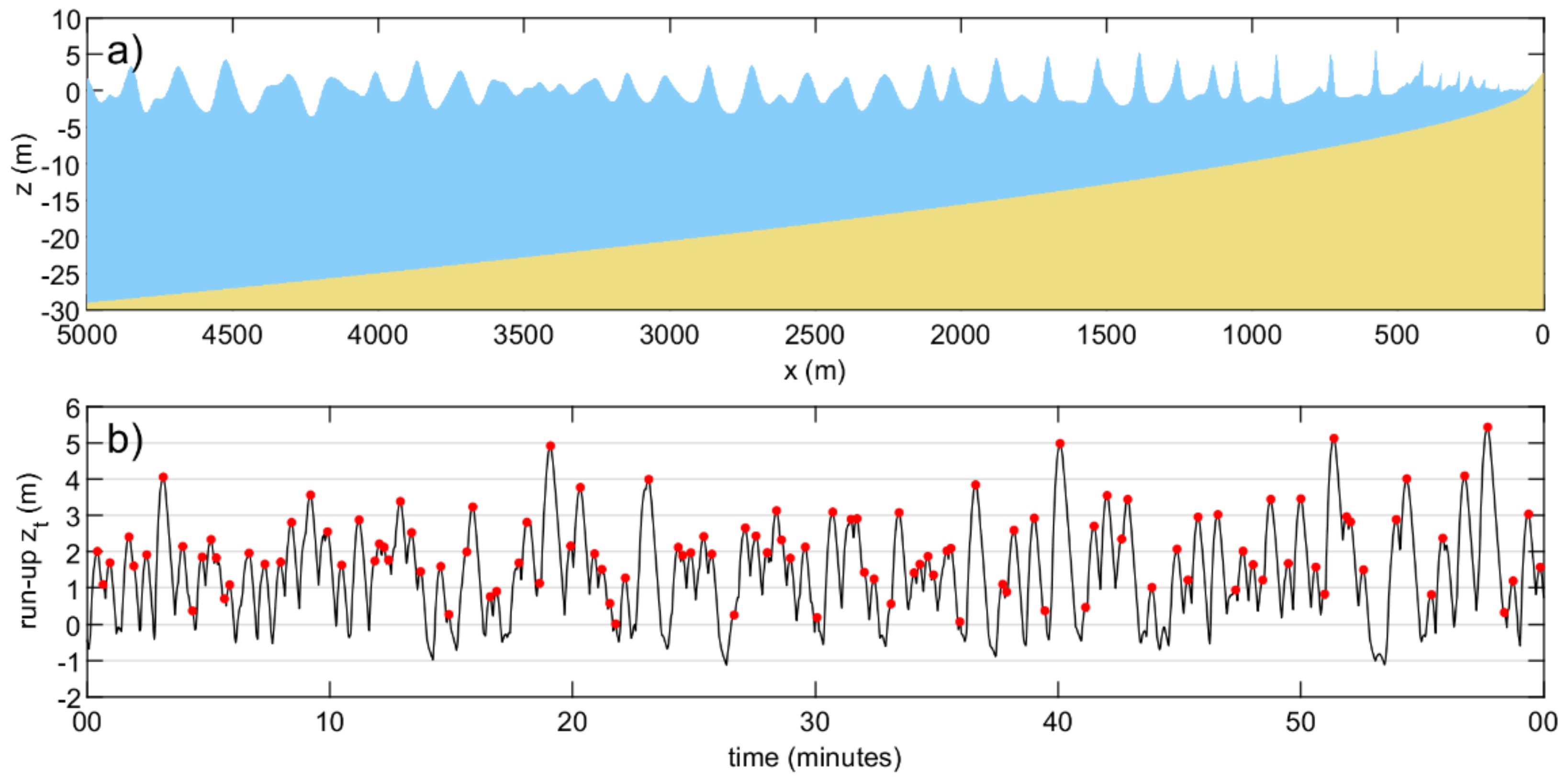
An example of XBeach-NH+ results is given in Figure 2, which shows a snapshot of cross-shore wave evolution for one of the simulations and the vertical run-up time series zt. Note that, whereas the offshore peak wave period Tp here is 12 s, the interval between the run-up peaks in Figure 2b is typically in the order of one minute, indicating that in this simulation, the run-up signal is dominated by lower-frequency infragravity wave motions.
For each simulation, the set-up zmean (Equation (1)) was calculated as the 3 h mean of the run-up elevation zt.
Like Stockdon [8], we calculated the significant swash height S (Equation (2)) from the run-up elevation zt similar to the calculation of significant wave height [21].
where PSD is the power spectral density and f is frequency.
The significant swash height in the incident band Sinc was calculated by summing only over frequencies greater than a cut-off frequency fc. Similarly, the swash height in the infragravity band SIG was determined by summing over frequencies below fc. Here, we used a cut-off frequency of half the peak frequency (Equation (3)):
Note that, in this regard, our method differs from [8] who use a constant cut-off frequency fc of 0.05 Hz.
The R2% run-up height (defined as the value exceeded by two percent of the run-up events) was determined by taking the 98th percentile of the peaks in the vertical run-up time series.
The derivation of the empirical relation for SIG was carried out in two steps (as shown in Section 3.3) and first requires an estimate of the incoming infragravity wave height Hin,IG and the infragravity period Tm-10,IG close to the shoreline. These were determined with the method presented in [21].
The aim of this study was to define zmean, Sinc, and SIG as the product of the deep-water wave height and some function of the dimensionless surf zone and beach Irribarren numbers, i.e., . The procedure for determining the Irribarren numbers is as follows.
For each simulation, we first estimated the breaking wave depth with Equation (4):
In this study, we assumed a constant wave breaking parameter γbr = 1.0. From there, the width Ws and mean slope of the surf zone tan βsz are determined with Equations (5) and (6):
The slope of the beach tan βb is one of the input variables and does not require calculation. The dimensionless surf similarity numbers for the surf zone ξsz and beach ξb are given by Equations (7) and (8).
Here, L0 is the deep-water wave length (Equation (9)):
3. Results
3.1. Set-Up zmean
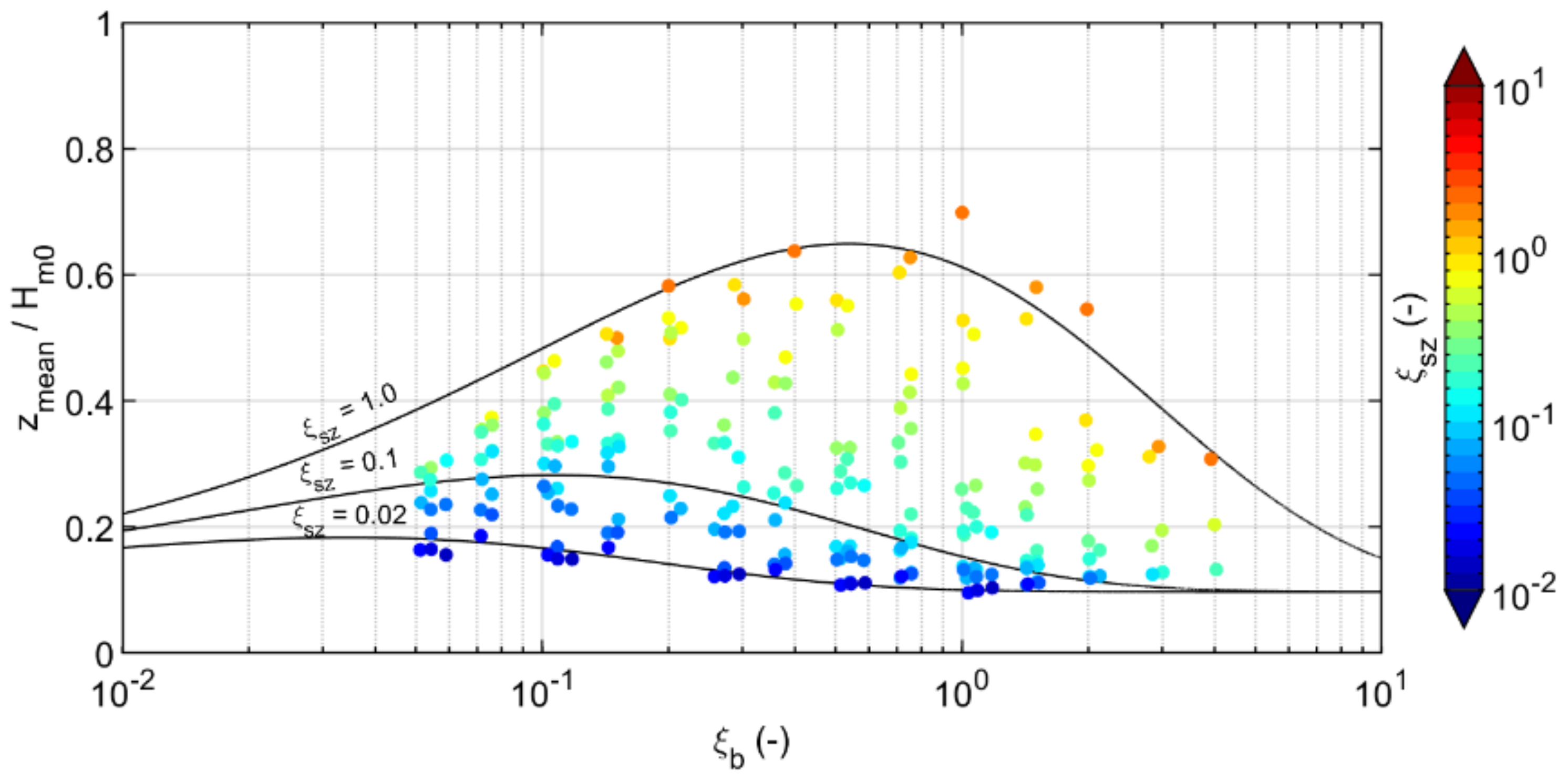
Qualitative analysis of the computed set-up zmean reveals a clear pattern (Figure 3) where the relative dimensionless set-up zmean/Hm0 always increases with increasing ξsz. The relation between zmean/Hm0 and ξb is more complicated. It shows that under dissipative beach conditions (i.e., low values of ξb), the relative set-up first increases with increasing ξb, and then, beyond a certain tipping point where beach conditions become reflective, starts to decrease. The model results indicate that the location of this tipping point is not fixed but depends on the surf zone conditions. Under dissipative conditions in the surf zone (ξsz < 0.1) the tipping point is located around ξb ≈ 0.05. For more reflective surf zone conditions (ξsz > 1.0), it is located around ξb ≈ 0.6.
It was experimentally found that this behavior can be described in the following form:
where A, B, C, D, and E are constants yet to be determined. After applying a non-linear least-square fitting procedure to determine their optimal values, the formulation for zmean is given by Equation (11):
The comparison between simulated set-up and Equation (11) (Figure 4) reveals very good agreement between the empirical fit and the XBeach-NH+ results.
3.2. Incident Run-Up Sinc
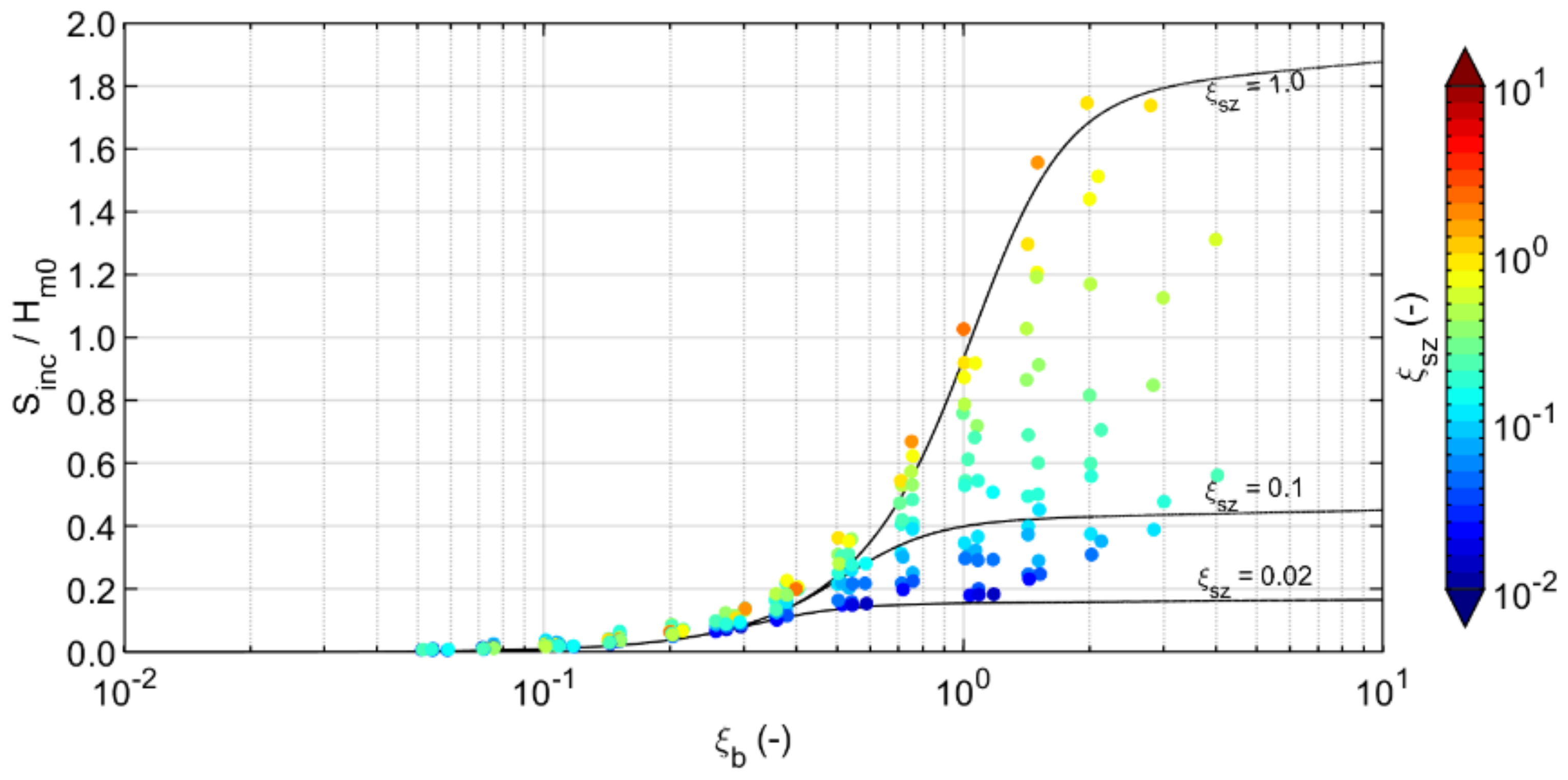
The relation between ξsz, ξb, and the relative dimensionless incident run-up Sinc/Hm0 is somewhat similar to that of the wave set-up (see Figure 5) described in the previous section. Sinc/Hm0 also increases with increasing ξsz values, and under dissipative beach conditions (i.e., low values of ξb), Sinc/Hm0 increases with increasing ξb, albeit much more rapidly than the relative wave set-up. Beyond the tipping point, Sinc/Hm0 remains fairly constant. Under very reflective conditions (ξb > ~3 and ξsz > ~1), the incident run-up approaches the standing wave limit (Sinc/Hm0 = 2).
It was again experimentally found that a good prediction of Sinc can be obtained when written in the following form:
The non-linear fitting procedure is now used to determine optimal values for the constants A, B, and C, resulting in the following empirical relation for Sinc:
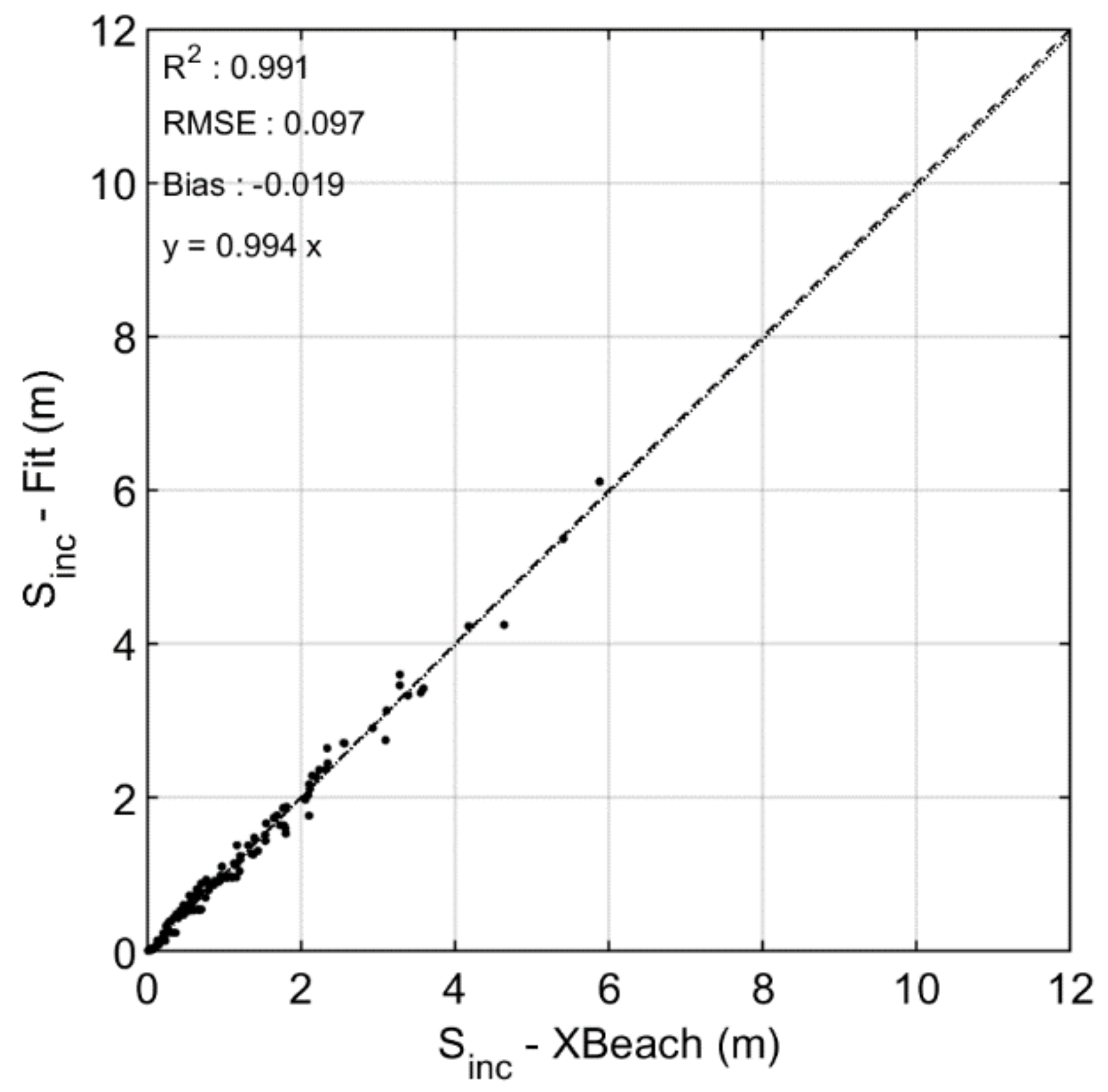
The comparison between simulated set-up and Equation (13) (Figure 6) reveals generally very good agreement between the empirical fit for Sinc and XBeach-NH+ results.
3.3. Infragravity Run-Up SIG
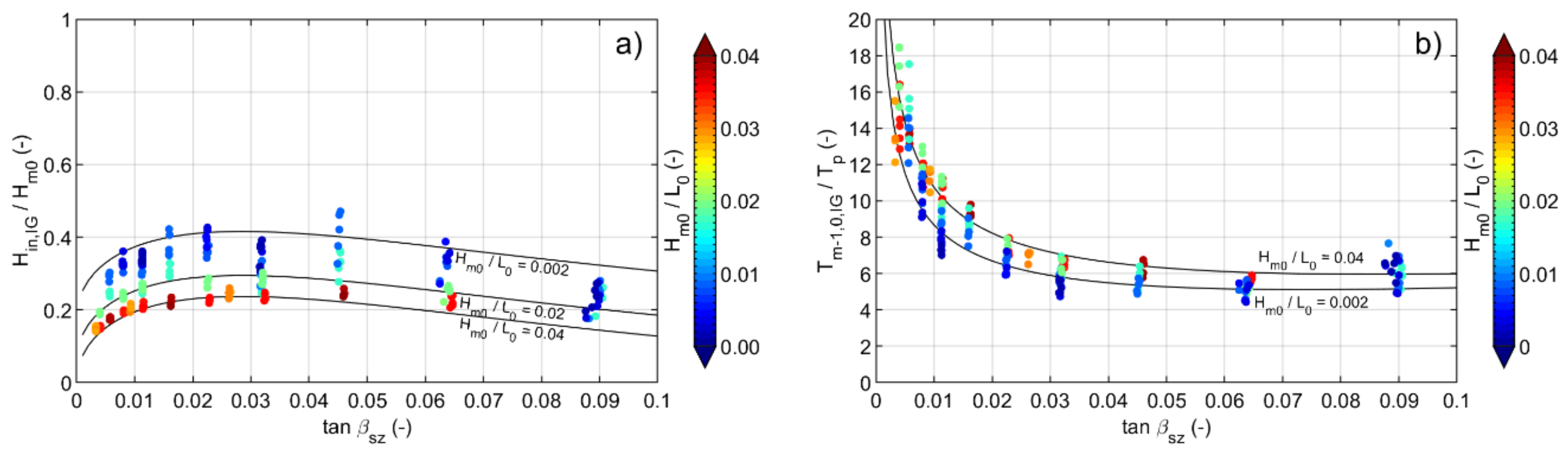
Inspection of the model results reveals that the frequency of infragravity waves at the shoreline strongly depends on the surf zone slope and, to a much lesser extent, the offshore wave steepness. For relatively steep surf zones (tan βs > 0.04), the Tm-10,in,IG wave period of the infragravity part of the power density spectrum is typically in the order of 5–7 times the deep-water peak wave period Tp. At milder sloping surf zones however, the model shows a shift of infragravity wave energy towards lower frequencies (Figure 7b). We believe that this shift is related to infragravity wave–wave interactions, but the exact physical process behind it remains to be investigated.
It is expected that the infragravity wave period at the shoreline is an important parameter for predicting the SIG run-up at the beach. A different strategy is therefore chosen to derive the formula for SIG in which this assumption is reflected. In the first step, we derive a relation for the incoming infragravity wave height Hin,IG at a location close to the shoreline, as well as the corresponding infragravity wave period Tm-10,in,IG. In the second step, we attempt to derive a relation for SIG, based on Hin,IG, Tm-10,in,IG, and the beach slope.
The nearshore location in the first step was chosen such that the bulk of the incident wave energy has dissipated, yet it is deep enough that it does not become dry at any time (and therefore yields a continuous time series of water levels and velocities). The latter is a requirement for accurately determining Hin,IG and Tm-10,in,IG. Here, we chose a point at which the still water depth equals one third of the offshore wave height Hm0. For a Dean profile and γbr = 1.0, the distance from the shore to this point equals 19.2 percent of the surf zone width.
After some experimentation, the following fits are found to estimate the incoming infragravity wave height (Equation (14)) and period (Equation (15)).
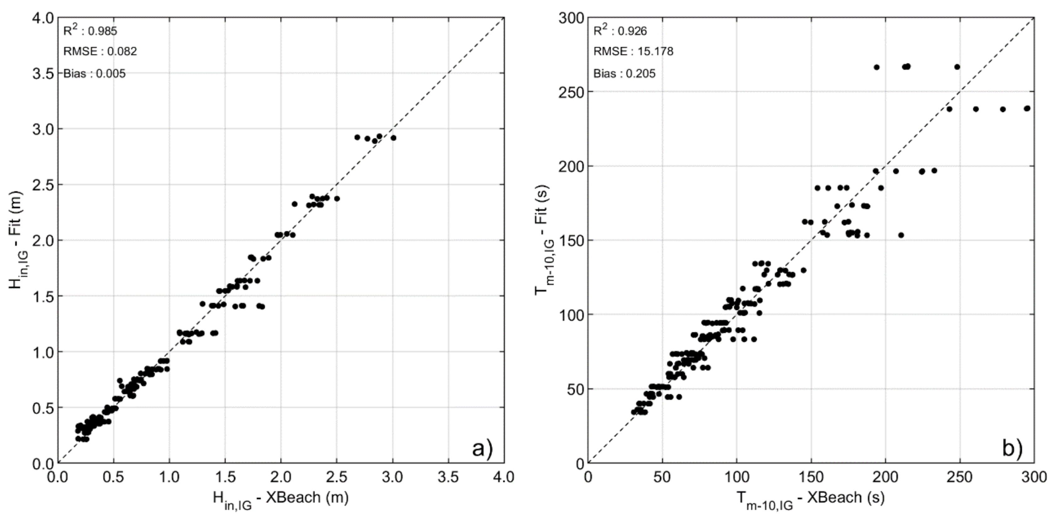
The comparison between simulation results and Equations (14) and (15) (Figure 8) reveals generally good agreement.
Rather than estimating the infragravity run-up with the original beach Irribarren number ξb which includes the deep-water steepness, we use an Irribarren number ξb,IG that is computed with the infragravity wave steepness near the shore (Equation (16)):
where the infragravity wave length Lin,IG is computed with Equation (17).
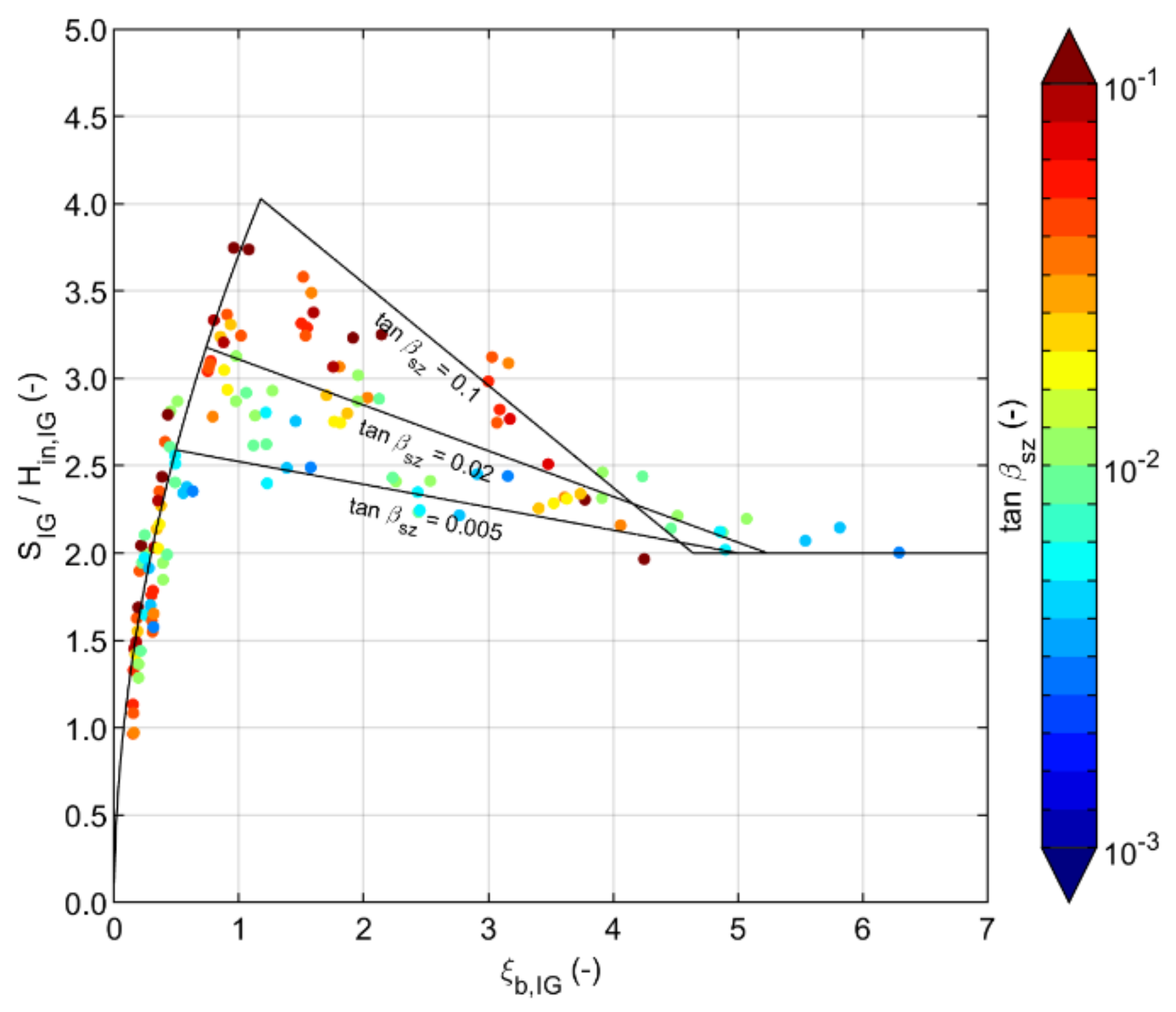
The response of the relative dimensionless infragravity run-up SIG/Hin,IG shows a clear distinction between dissipative and reflective beach conditions (Figure 9). Under dissipative beach conditions (i.e., low values of ξb,IG), the relative run-up first increases with increasing ξb,IG, and then, beyond a tipping point , starts to linearly decrease with increasing ξb,IG. We also see that SIG cannot be properly described as a function of Hin,IG and ξb,IG alone. For more reflective conditions on the beach, a dependency on the surf zone slope βsz is found which affects the boundary between the dissipative and reflective regimes. This dependency can likely be attributed to the fact that in steeper surf zones, the incident wave energy is relatively higher at the location where the incoming infragravity wave height is determined (i.e., at a depth of one third the offshore wave height). Shoreward of this location, a portion of the remaining short-wave energy is still converted to infragravity energy, thereby increasing the infragravity run-up at the beach. Under very reflective conditions (ξb,IG > ~4), the infragravity run-up approaches the standing wave limit (SIG/Hin,IG = 2).
After determining the optimal values for the constants A, B, C, D, and E, with a non-linear fitting procedure, the full set of equations is given by Equations (21)–(23).
where:
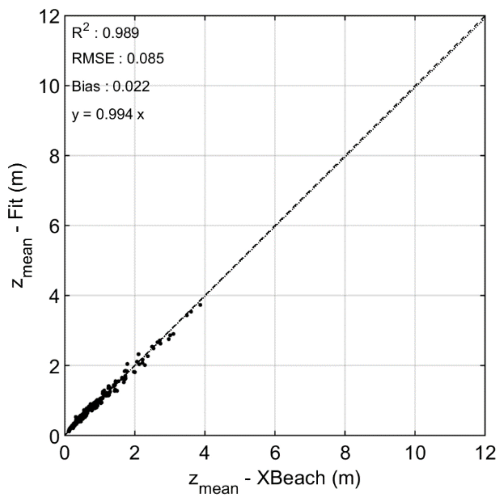
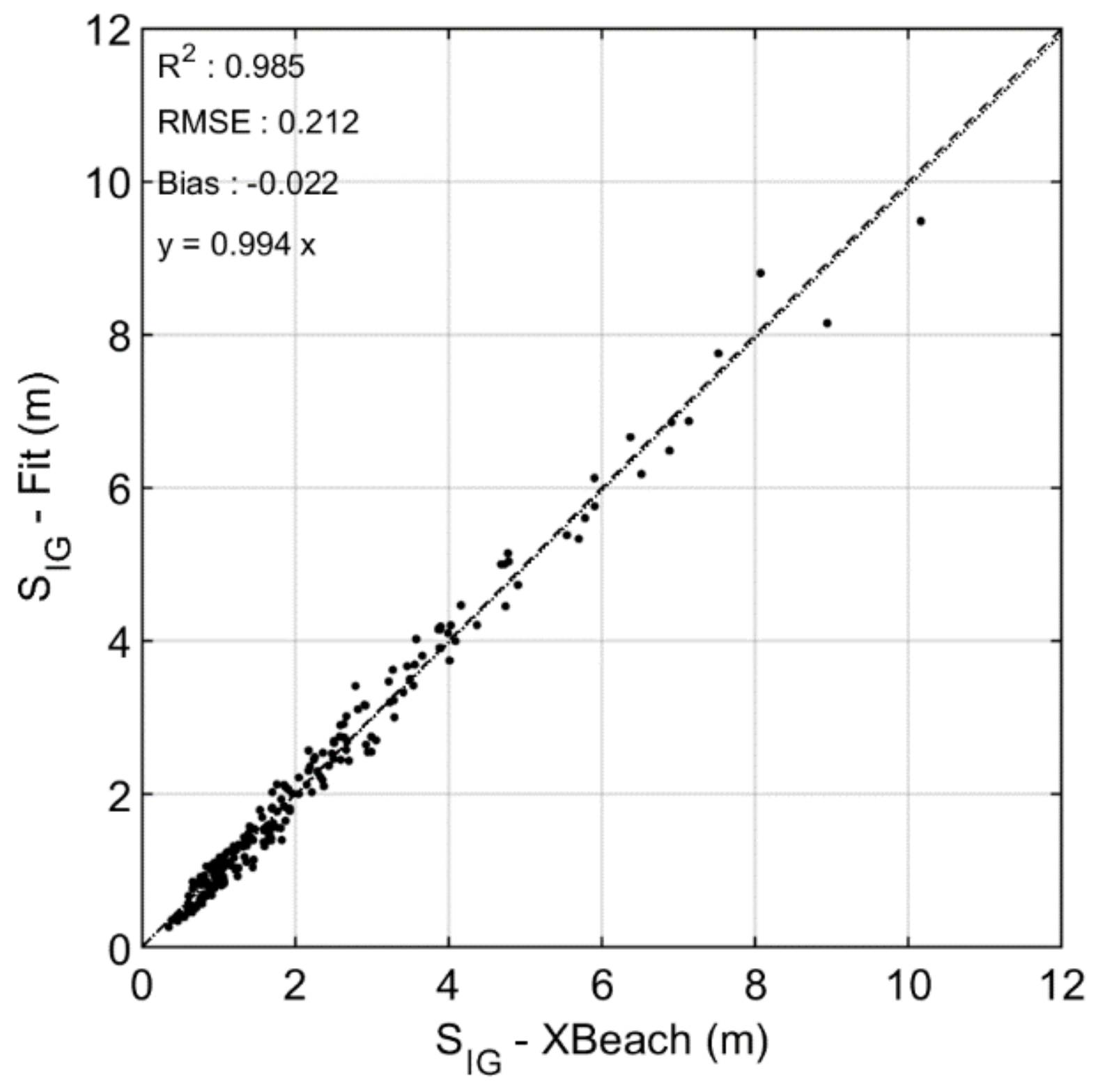
The comparison of SIG obtained from XBeach-NH+ versus the outcome of Equations (14)–(23) reveals good agreement between the numerical simulation and the empirical formulations (Figure 10).
3.4. Run-Up R2%
With satisfactory estimates for zmean, SIG, and Sinc, it is now possible to derive a formulation for the total run-up R2%. Initially, we attempted to use a formulation similar to the one used by Stockdon [8]:
Here, R2% is the run-up computed by the XBeach-NH+ model and zmean, SIG, and Sinc are computed with Equations (11), (13) and (14)–(23), respectively. The optimal values for the constants A, B, and C can be determined using a non-linear fitting procedure.
It was however found that the inclusion of ξsz and ξb in the estimation of R2% yielded a significant performance improvement. Eventually, the best fit that was found for R2% is given by Equation (25).
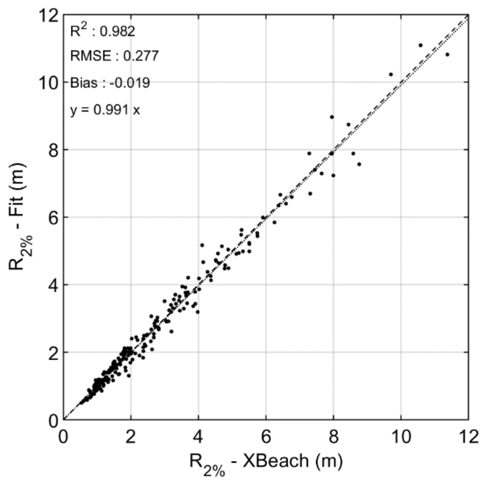
There is generally good agreement between run-up values from the XBeach-NH+ simulations and those computed with Equation (25) (Figure 11).
3.5. Angle of Incidence
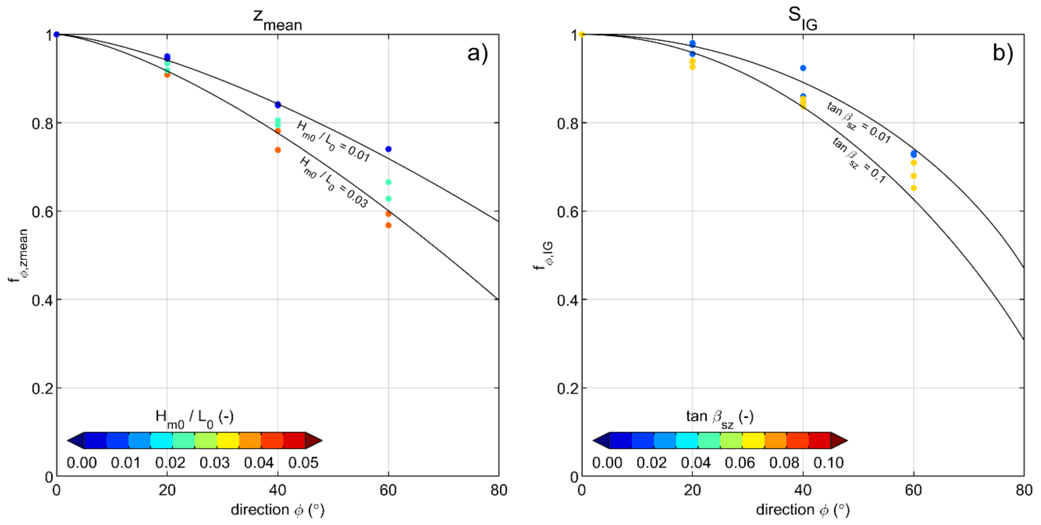
A limited set of 2D simulations were carried out to determine the reduction factors for the offshore wave angle φ with respect to the coast. Due to the strongly increased computational effort required to run the 2D simulations, the 2D runs were only performed with on offshore wave height Hm0 of 2.0 m. Furthermore, the beach slope tan βb was kept constant at 0.05. Model input parameters were kept identical to those in the 1D simulations. The 2D model was forced at the boundaries with waves coming in at angles φ of 0, 20, 40, and 60 degrees. The alongshore extent and resolution of the 2D model was 1 km and 1 m, respectively. The reduction factors were determined with:
where S2D and S2D,0 are zmean, Sinc, or SIG from the 2D simulations with oblique (φ > 0), and normal incident wave (φ = 0), respectively. The reduction factors are to be applied to Equations (11), (13), (21) and (22) before computing the total run-up with Equation (25).
The incident wave run-up height Sinc was found to be insensitive to the incident wave angle. We therefore used fφ,inc = 1.0. The set-up zmean and infragravity run-up height SIG, however, showed a clear decrease with increasing wave angle φ (Figure 12). The reduction effect of the wave angle on zmean was stronger for steeper offshore waves (Figure 12a), whereas the reduction of the infragravity run-up SIG was found to be greater for relatively steep surf zones (Figure 12b).
A good match for fφ,zmean and fφ,inc (see Figure 13) was found when the reduction factors for set-up and SIG are estimated with Equations (27) and (28):
3.6. Directional Spreading
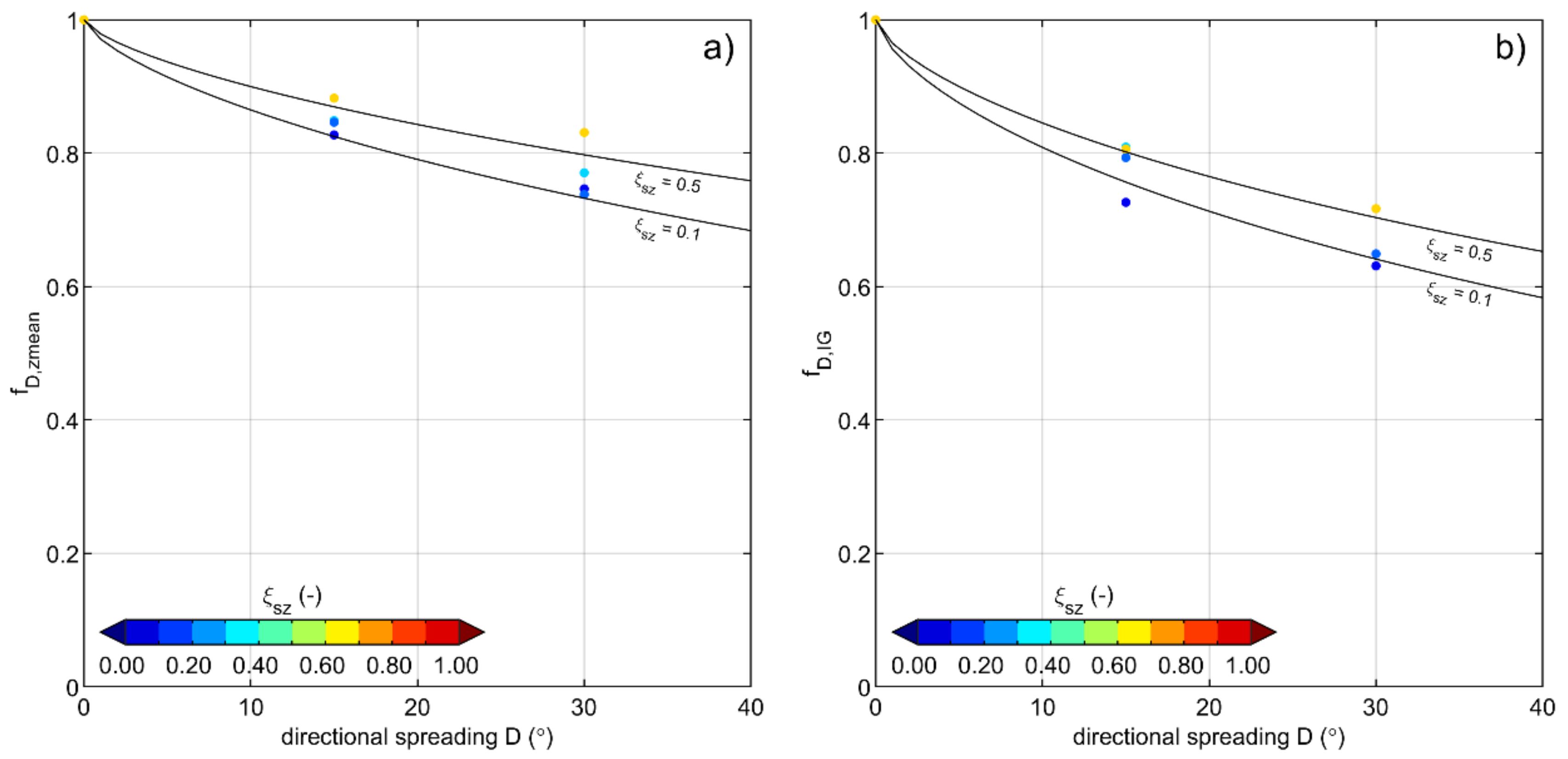
A similar approach was used to determine reduction factors for directional spreading D (here defined as the directional standard deviation in degrees), but rather than varying the angle of incidence, we varied the directional spreading D in the offshore wave spectra that make up the offshore boundary conditions, using values of 0, 15, and 30 degrees. Similar to the angle of incidence, the incident wave run-up height Sinc was found to be insensitive to the directional spreading. We therefore used fD,inc = 1.0. The set-up and infragravity run-up, however, both decrease with increasing directional spreading (Figure 14). The reduction effect for both zmean and SIG was enhanced under more dissipative conditions in the surf zone (lower values of ξsz). Qualitatively similar results were obtained by [22].
The largest effect of directional spreading was found on the infragravity run-up, where SIG can be reduced by over 40 percent. The best fit is found when the reduction factors are estimated with Equations (29) and (30) (see also Figure 15).
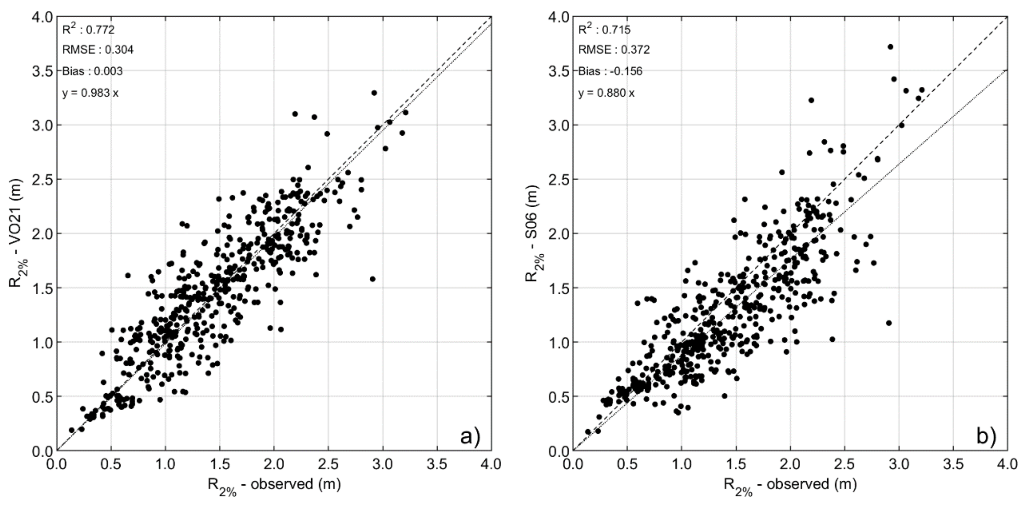
3.7. Validation
Until this point, the data to derive the empirical relations have all been obtained from hydrodynamic model results. Here, we now validate the results against field observations, using the video-derived run-up data collected by Stockdon [8], hereafter referred to as S06. As the original S06 data do not include information on offshore wave angle and directional spreading, these were obtained from WAVEWATCH III re-analysis data by NOAA [23]. Surf zone profiles were obtained by digitizing the bathymetry profiles provided by S06. Tide levels at each data point were computed from the TPXO 7.2 database [24].
To compute the run-up, the time-varying surf zone slope was computed separately for each data point in the S06 dataset. This was conducted with Equations (4)–(6), using the surf zone depth profile and including the tide level. The beach steepness βb was taken from the S06 dataset.
The scatter plot in Figure 16a shows the comparison between observed and computed R2% values (using Equation (25)). For reference, the results of the S06 formulations are shown in Figure 16b. The results with the empirical relations from the present study (VO21) generally compare well with the observations. The VO21 error statistics are significantly better than those from S06. In particular, the VO21 formulations do not suffer from the negative bias seen in S06. Furthermore, the R2 correlation coefficient of VO21 (0.772) is higher than that of SO6 (0.715), and the root-mean-square error is lower (0.304 vs. 0.372 m). It should be noted here that there is a considerable amount of scatter in the S06 run-up data. The scatter can to some extent be explained by the relatively short 17 min video observation intervals which introduce uncertainty in the run-up estimates. The uncertainty in infragravity run-up estimates may be as high as 65% [25].
The performance of the VO21 results and comparison to S06 is further discussed in the next section.
4. Discussion and Conclusions
The empirical relations described in Section 3.1, Section 3.2, Section 3.3 and Section 3.4 are able to accurately reproduce the run-up characteristics computed by the XBeach-NH+ 1D profile models. Furthermore, when combined with the reduction factors for incident wave angle (Section 3.5) and directional spreading (Section 3.6), the use of these new relations results in improved error statistics compared to the S06 relations, using the same dataset. In particular, the new relations do not suffer from the negative bias that is seen in the S06 relations. On the one hand, this result is not entirely surprising, as the method presented here takes in more forcing data (tides, surf zone slope, incident angle, and directional spreading) than was used in the S06 formulations. On the other hand, it must be noted that the new VO21 relations were derived from an entirely different dataset obtained from numerical hydrodynamic model results, whereas the S06 formulations are the result of a direct fit of the field observation data. Furthermore, the model results were obtained from a wider range of wave and topographic conditions (see Table 2), with the exception of somewhat lower minimum wave heights and periods in the field data. It is therefore to be expected that the VO21 formulations are valid over a wider range of conditions than S06, and in particular, under extreme wave events which are not included in the field data.
It should be noted here that many alternative run-up formulations have been derived in recent years. For a thorough overview, we refer to [13]. A number of these formulas have been parameterized with larger and/or different field datasets than S06, and some have shown better performance than S06. The main reason for quantitively comparing VO21 only to the S06 relations lies in the fact that S06 is the only formulation that has been trained solely with our validation dataset (i.e., the video-derived field data collected by [8]). Furthermore, S06 remains at the time of writing the most known and applied formula in the engineering community.
Whereas most existing predictors in [13] include only one slope (typically the swash zone slope), VO21 considers both the surf zone slope (which varies with the tide) and the swash slope. Another important feature of VO21 is that it distinguishes between dissipative and reflective conditions in both the surf zone and on the beach. The fact that these effects are not included in many other predictors may explain why previous studies did not see an improvement of their infragravity run-up predictions by including beach slope (e.g., [8,12,22]). In the present study, there is a clear response of the infragravity run-up height to changes in the beach slope. We see a positive relation between Irribarren numbers and both set-up and wave run-up under dissipative conditions at the beach. Beyond a certain tipping point, however, set-up and infragravity run-up start to decrease with increasing Irribarren numbers, and incident run-up remains constant. Other parameters that have been shown to be important in this study, and which are typically not included in existing relations, are the incident wave angle and directional spreading of the offshore wave conditions.
The effect of excluding the above-mentioned parameters in our validation against the field data have been investigated. The results of this sensitivity test are presented in Table 3. Exclusion of the vertical tide results in slightly poorer performance (with slightly decreased R2 and increased RMSE). Not including offshore wave angle (φ = 0) and particularly the directional spreading (D = 0) leads to slightly lower correlation R2 with the data and introduces a strong positive bias. The greatest effect is however seen when excluding the effect of the surf zone slope. This was investigated by maintaining a constant surf zone slope of 0.046 (the mean of all values computed for the S06 dataset). Not including the effect of the surf zone slope significantly reduces the R2, and increases the RMSE by 27 percent, again highlighting the relative importance of this parameter.
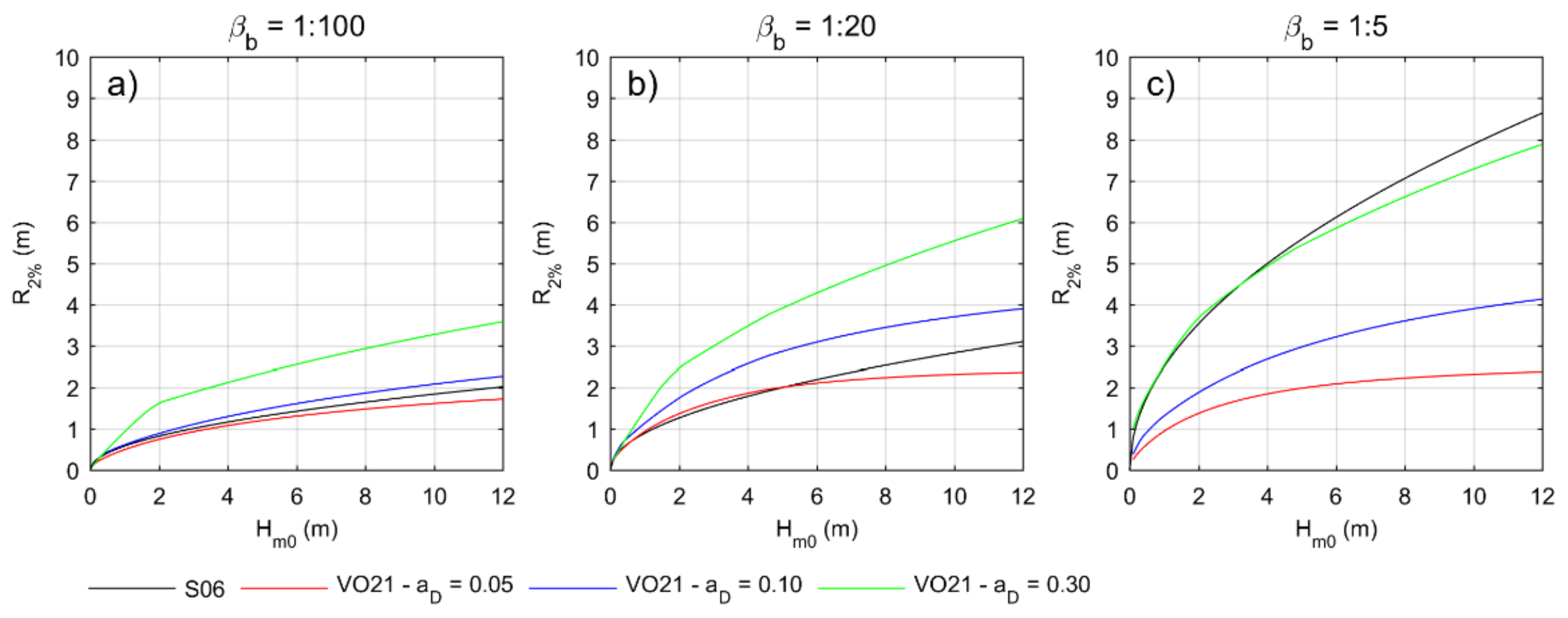
In Figure 17, R2% predictions from VO21 are shown for mild (18a), intermediate (18b), and steep (18c) beach and mild (red), intermediate (blue) and steep (green) underwater slopes. The S06 formula results, which do not include the surf zone slope, are shown in black. The figure highlights the importance of the effect of the underwater steepness on run-up (compare the red, blue, and green lines). Furthermore, it suggests that S06 yields significantly lower run-up during large wave events (compared to VO21) at intermediate and steep underwater slopes, except for the case of very steep beach slopes.
The fact that VO21 requires more input data can of course also be a disadvantage, in particular when such data are not available. Here, we list recommendations when some of the data are missing. Typically, tide data can always be obtained, either from nearby tide gauges, or from global tide models, such as [24]. The incident wave angle and directional spreading can be obtained from nearby directional wave buoys, or from global wave re-analyses or forecasts. Setting either parameter to 0.0 typically leads to an overestimation of the run-up and is therefore not recommended. Tests with the validation dataset reveal a zero bias between VO21 predictions and observations when incident wave direction and spreading are set to 29 degrees and 25 degrees, respectively. When the surf zone profile is not known, one can estimate a Dean slope parameter aD by, e.g., estimating the distance L10 between the shoreline and the 10 m depth contour from a global bathymetry dataset, such as [26]. The Dean parameter aD can then be computed with . From there, the surf zone slope can be computed with Equations (4)–(7).
The VO21 formulations are not valid along reef-fringed coastlines. Nor are they likely valid on gravel beaches where permeability may have a significant effect on run-up elevations [27].
Some, potentially important, parameters have not been taken into account in VO21. These include the effects on vertical run-up of bed roughness, the presence of breaker bars, and alongshore non-uniformities (e.g., rip channels). Furthermore, the effect of the offshore wave frequency spectrum has not been investigated. Guza and Feddersen [22] showed that R2% wave run-up tends to increase with increasing frequency spread. Here, however, we used a JONSWAP spectrum with a constant peak enhancement factor of 3.3. Further work is required to include the above-mentioned effects.
It is recommended that the VO21 relations are further validated against more extensive datasets, in particular datasets with more extreme conditions. Although its predictions now closely match the numerical model results under extreme conditions (Hm0 > 4 m), we have not performed a validation of VO21 against field data under such conditions, as these are not available in the validation dataset [8].
Finally, the present study shows a relation between the surf zone slope on the infragravity wave period at the shoreline. For relatively steep surf zones, the infragravity wave period Tm-10,IG is typically in the order of 5–7 times the deep-water peak wave period Tp. At milder sloping surf zones, however, this study shows a shift of infragravity wave energy towards lower frequencies. The cause of this phenomenon remains to be further investigated.
Author Contributions
Methodology and writing, M.v.O.; writing—review and editing, D.R. and A.v.D. All authors have read and agreed to the published version of the manuscript.
Funding
This work was funded in part by the Office of Naval Research through Grant N00014-21-1-2235, the Deltares Strategic Research Program “Natural Hazards” and IHE Delft internal funding.
Institutional Review Board Statement
Not applicable.
Informed Consent Statement
Not applicable.
Data Availability Statement
The Stockdon [8] dataset may be downloaded from https://pubs.usgs.gov/ds/602/. (access date: 25 February 2020).
Conflicts of Interest
The authors declare no conflict of interest. The funders had no role in the design of the study; in the collection, analyses, or interpretation of data; in the writing of the manuscript, or in the decision to publish the results.
References
- Vatvani, D.; Zweers, N.C.; van Ormondt, M.; Smal, A.J.; de Vries, H.; Makin, V.K. Storm surge and wave simulations in the Gulf of Mexico using a consistent drag relation for atmospheric and storm surge models. Nat. Hazards Earth Syst. Sci. 2012, 12, 2399–2410. [Google Scholar] [CrossRef]
- Westerink, J.J.; Feyen, J.C.; Atkinson, J.H.; Roberts, H.J.; Kubatko, E.J.; Luettich, R.A.; Dawson, C.; Powell, M.D.; Dunion, J.P.; Pourtuheri, H. A basin- to channel-scale unstructured grid hurricane storm surge model applied to southern Louisiana. Mon. Weather Rev. 2008, 136, 833–864. [Google Scholar] [CrossRef]
- Jelesnianski, C.P.; Chen, J.; Shaffer, W.A. SLOSH: Sea, Lake, and Overland Surges from Hurricanes; NOAA Technical Report NWS 48; National Oceanic and Atmospheric Administration, U.S. Department of Commerce: Silver Spring, MD, USA, 1992; pp. 1–71. [Google Scholar]
- Longuet-Higgins, M.S.; Stewart, R.W. Radiation stress and mass transport in surface gravity waves with application to “surf beats”. J. Fluid Mech. 1962, 13, 481–504. [Google Scholar] [CrossRef]
- Mayo, T.; Lin, N. The Effect of the Surface Wind Field Representation in the Operational Storm Surge Model of the National Hurricane Center. Atmosphere 2019, 10, 193. [Google Scholar] [CrossRef] [Green Version]
- Roelvink, F.E.; Storlazzi, C.D.; van Dongeren, A.R.; Pearson, S.G. Coral Reef Restorations Can Be Optimized to Reduce Coastal Flooding Hazards. Front. Mar. Sci. 2021, 8, 653945. [Google Scholar] [CrossRef]
- Lashley, C.H.; Roelvink, D.; van Dongeren, A.; Buckley, M.L.; Lowe, R.J. Nonhydrostatic and surfbeat model predictions of extreme wave run-up in fringing reef environments. Coast Eng. 2018, 137, 11–27. [Google Scholar] [CrossRef] [Green Version]
- Stockdon, H.F.; Holman, R.A.; Howd, P.A.; Sallenger, A.H., Jr. Empirical parameterization of setup, swash and runup. Coast. Eng. 2006, 53, 573–588. [Google Scholar] [CrossRef]
- Stockdon, H.F.; Doran, K.J.; Thompson, D.M.; Sopkin, K.L.; Plant, N.G.; Sallenger, A.H. National assessment of hurricane-induced coastal erosion hazards—Gulf of Mexico. U.S. Geological Survey 2012-1084, 51p. [CrossRef] [Green Version]
- Holman, R.A. Extreme value statistics for wave run-up on a natural beach. Coast. Eng. 1986, 9, 527–544. [Google Scholar] [CrossRef]
- Ruggiero, P.; Komar, P.D.; McDougal, W.G.; Marra, J.J.; Beach, R.A. Wave runup, extreme water levels and erosion properties backing beaches. J. Coast. Res. 2001, 17, 407–419. [Google Scholar]
- Senechal, N.; Coco, G.; Bryan, K.R.; Holman, R.A. Wave runup during extreme storm conditions. J. Geophys. Res. 2011, 116. [Google Scholar] [CrossRef] [Green Version]
- Gomes da Silva, P.; Coco, G.; Garnier, R.; Klein, A.H.F. On the prediction of runup, setup and swash on beaches. Earth-Sci. Rev. 2020, 204, 103148. [Google Scholar] [CrossRef]
- Cheriton, O.M.; Storlazzi, C.D.; Rosenberger, K.J. Observations of wave transformation over a fringing coral reef and the importance of low-frequency waves and offshore water levels to runup, overwash, and coastal flooding. J. Geophys. Res. Oceans 2016, 121, 3121–3140. [Google Scholar] [CrossRef] [Green Version]
- Stockdon, H.F.; Thompson, D.M.; Plant, N.G.; Long, W.J. Evaluation of wave runup predictions from numerical and parametric models. Coast. Eng. 2014, 92, 1–11. [Google Scholar] [CrossRef]
- Roelvink, J.A.; Reniers, A.J.H.M.; Van Dongeren, A.R.; Van Thiel de Vries, J.; McCall, R.T.; Lescinski, J. Modelling storm impacts on beaches, dunes and barrier islands. Coast. Eng. 2009, 56, 1133–1152. [Google Scholar] [CrossRef]
- Roelvink, D.; McCall, R.; Mehvar, S.; Nederhoff, K.; Dastgheib, A. Improving predictions of swash dynamics in XBeach: The role of groupiness and incident-band runup. Coast. Eng. 2018, 134, 103–123. [Google Scholar] [CrossRef]
- De Ridder, M.P.; Smit, P.B.; van Dongeren, A.R.; McCall, R.T.; Nederhoff, K.; Reniers, A.J. Efficient two-layer non-hydrostatic wave model with accurate dispersive behaviour. Coast. Eng. 2021, 164, 103808. [Google Scholar] [CrossRef]
- Iribarren, R.; Nogales, C. Protection of ports. In Proceedings of the PIANC World Congress, Lisbon, Portugal, 10–19 September 1949; p. 31. [Google Scholar]
- Dean, R.G. Equilibrium beach profiles: Characteristics and applications. J. Coast. Res. 1991, 7, 53–84. [Google Scholar]
- Guza, R.T.; Thornton, E.B.; Holman, R.A. Swash on steep and shallow beaches. Coast. Eng. Proc. 1984, 1, 708–722. [Google Scholar] [CrossRef] [Green Version]
- Guza, R.T.; Feddersen, F. Effect of wave frequency and directional spread on shoreline runup. Geophys. Res. Lett. 2012, 39. [Google Scholar] [CrossRef] [Green Version]
- Tolman, H.L. User manual and system documentation of WAVEWATCH-III version 1.18. In NOAA/NWS/NCEP/OMB Technical note 166; NOAA/NWS/NCEP: College Park, MD, USA, 1999; p. 110. [Google Scholar]
- Egbert, G.D.; Erofeeva, S.Y. Efficient inverse modeling of barotropic ocean tides. J. Atmos. Oceanic Technol. 2002, 19, 183–204. [Google Scholar] [CrossRef] [Green Version]
- Fiedler, J.W.; Smit, P.B.; Brodie, K.L.; McNinch, J.; Guza, R.T. Numerical modeling of wave runup on steep and mildly sloping natural beaches. Coast. Eng. 2018, 131, 106–113. [Google Scholar] [CrossRef]
- Olson, C.J.; Becker, J.J.; Sandwell, D.T. A New Global Bathymetry Map at 15 Arcsecond Resolution for Resolving Seafloor Fabric: SRTM15_PLUS; AGU Fall Meeting Abstracts: Washington, DC, USA, 2014. [Google Scholar]
- Poate, T.G.; McCall, R.T.; Masselink, G. A new parameterisation for runup on gravel beaches. Coast. Eng. 2016, 117, 176–190. [Google Scholar] [CrossRef] [Green Version]
Figure 1.
Cross−shore profiles for Hm0 = 2 m, Tp = 12 s, tan βb = 0.10, and four values of aD (0.05, 0.10, 0.20, and 0.30).
Figure 1.
Cross−shore profiles for Hm0 = 2 m, Tp = 12 s, tan βb = 0.10, and four values of aD (0.05, 0.10, 0.20, and 0.30).

Figure 2.
Snapshot of cross−shore wave evolution (a) and vertical run-up time series over 1 h (b) for Hm0 = 8 m, Tp = 12 s, aD = 0.1, and tan βs = 0.1 zoomed in to first 5 km from the shoreline. Peaks in the vertical run-up signal (b) indicated by red dots.
Figure 2.
Snapshot of cross−shore wave evolution (a) and vertical run-up time series over 1 h (b) for Hm0 = 8 m, Tp = 12 s, aD = 0.1, and tan βs = 0.1 zoomed in to first 5 km from the shoreline. Peaks in the vertical run-up signal (b) indicated by red dots.

Figure 3.
Relative set-up zmean/Hm0 as a function of ξsz and ξb. Solid lines are the empirical fit for ξsz = 0.02, ξsz = 0.10, and ξsz = 1.0.
Figure 3.
Relative set-up zmean/Hm0 as a function of ξsz and ξb. Solid lines are the empirical fit for ξsz = 0.02, ξsz = 0.10, and ξsz = 1.0.

Figure 4.
Comparison of XBeach-NH+ results and empirical fit for set-up zmean. Dashed line indicates unity (y = x).
Figure 4.
Comparison of XBeach-NH+ results and empirical fit for set-up zmean. Dashed line indicates unity (y = x).

Figure 5.
Relative incident run-up Sinc/Hm0 as a function of ξs and ξb. Solid lines are the empirical fit for ξsz = 0.02, ξsz = 0.10, and ξsz = 1.0.
Figure 5.
Relative incident run-up Sinc/Hm0 as a function of ξs and ξb. Solid lines are the empirical fit for ξsz = 0.02, ξsz = 0.10, and ξsz = 1.0.

Figure 6.
Comparison of XBeach-NH+ and empirical fit for incident run-up Sinc. Dashed line indicates unity (y = x).
Figure 6.
Comparison of XBeach-NH+ and empirical fit for incident run-up Sinc. Dashed line indicates unity (y = x).

Figure 7.
Effect of surf zone slope and offshore wave steepness on incoming infragravity wave height (a) and infragravity wave period Tm-10,in,IG (b) near the shoreline. Solid lines are the empirical fit for various offshore wave steepness.
Figure 7.
Effect of surf zone slope and offshore wave steepness on incoming infragravity wave height (a) and infragravity wave period Tm-10,in,IG (b) near the shoreline. Solid lines are the empirical fit for various offshore wave steepness.

Figure 8.
Comparison of XBeach-NH+ and empirical fit for incoming infragravity wave height (a) and period Tm-01,in,IG (b) near the shoreline. Dashed line indicates unity (y = x).
Figure 8.
Comparison of XBeach-NH+ and empirical fit for incoming infragravity wave height (a) and period Tm-01,in,IG (b) near the shoreline. Dashed line indicates unity (y = x).

Figure 9.
Relative infragravity run-up SIG/Hin,IG as a function of ξb,IG and tan βsz. Solid lines are the empirical fit for tan βsz = 0.005, tan βsz = 0.02, and tan βsz = 0.1.
Figure 9.
Relative infragravity run-up SIG/Hin,IG as a function of ξb,IG and tan βsz. Solid lines are the empirical fit for tan βsz = 0.005, tan βsz = 0.02, and tan βsz = 0.1.

Figure 10.
Comparison of XBeach-NH+ and empirical fit for infragravity run-up SIG. Dashed line indicates unity (y = x).
Figure 10.
Comparison of XBeach-NH+ and empirical fit for infragravity run-up SIG. Dashed line indicates unity (y = x).

Figure 11.
Comparison of XBeach-NH+ and the empirical relation (Equation (25)) for run-up R2%. Dashed line indicates unity (y = x).
Figure 11.
Comparison of XBeach-NH+ and the empirical relation (Equation (25)) for run-up R2%. Dashed line indicates unity (y = x).

Figure 12.
Computed wave angle reduction factors fφ for set-up (a) and infragravity run-up (b). Solid lines in (a) show the empirical fit with offshore wave steepness of 0.01 and 0.03. Solid lines in (b) show the empirical fit surf zone slope of 0.01 and 0.1.
Figure 12.
Computed wave angle reduction factors fφ for set-up (a) and infragravity run-up (b). Solid lines in (a) show the empirical fit with offshore wave steepness of 0.01 and 0.03. Solid lines in (b) show the empirical fit surf zone slope of 0.01 and 0.1.

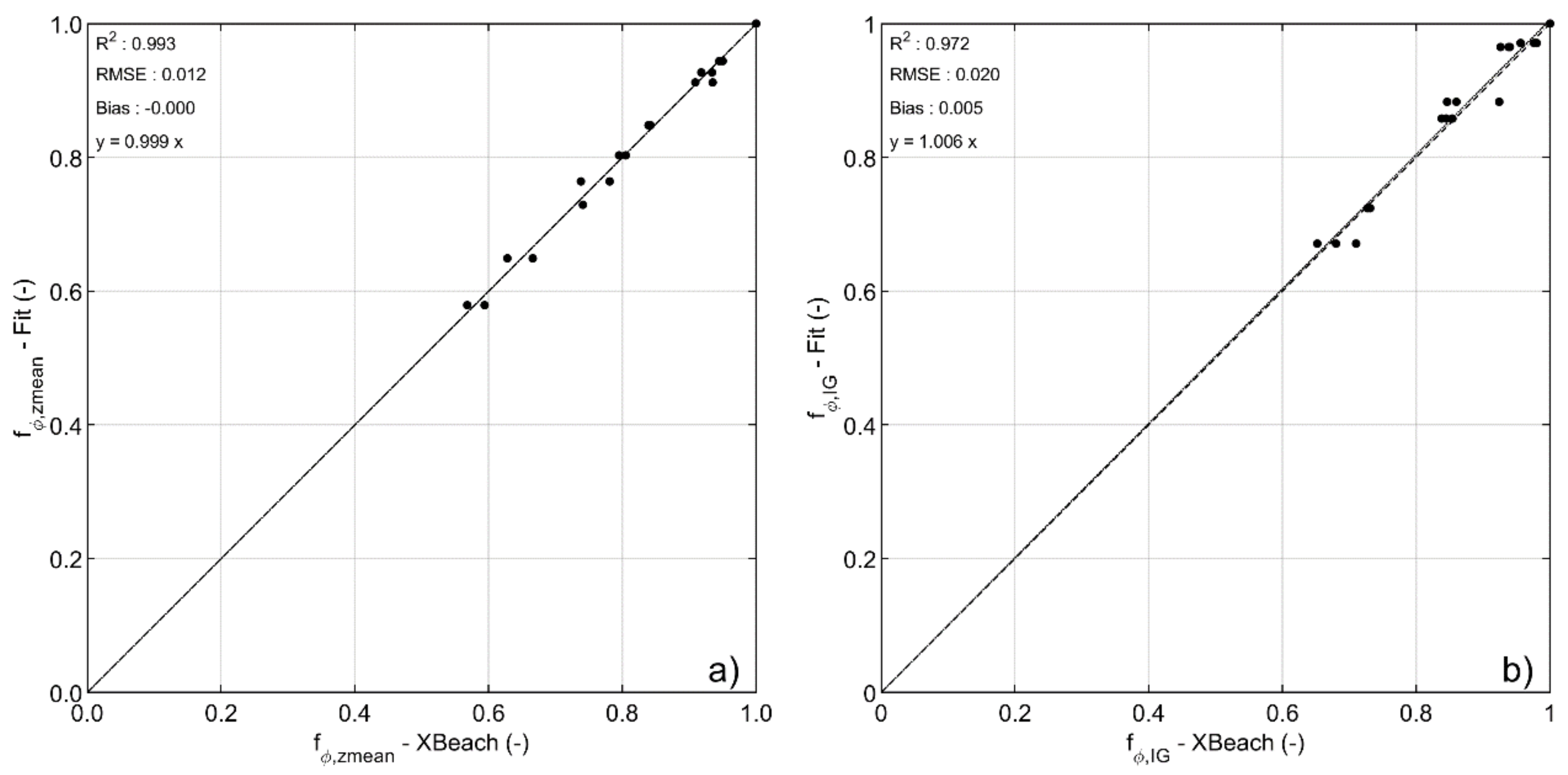
Figure 13.
Comparison of simulated and computed wave angle reduction factors fφ for set-up (a) and infragravity run-up (b). Dashed line indicates unity (y = x).
Figure 13.
Comparison of simulated and computed wave angle reduction factors fφ for set-up (a) and infragravity run-up (b). Dashed line indicates unity (y = x).

Figure 14.
Computed directional spreading reduction factors fD for set-up (a) and infragravity run-up (b). Solid lines show the empirical fit with ξsz of 0.1 and 0.5.
Figure 14.
Computed directional spreading reduction factors fD for set-up (a) and infragravity run-up (b). Solid lines show the empirical fit with ξsz of 0.1 and 0.5.

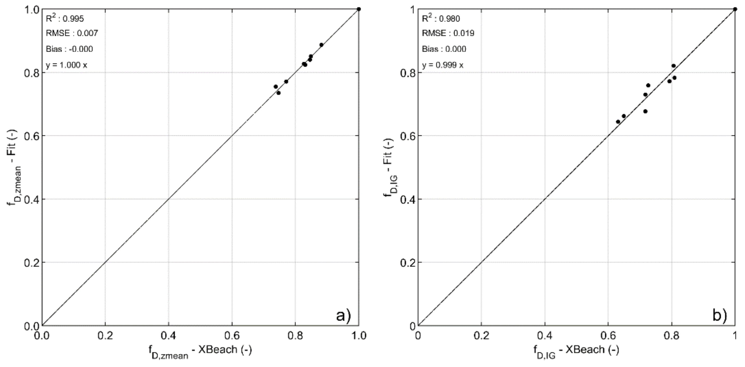
Figure 15.
Comparison of simulated and computed directional spreading reduction factors fD for set-up (a) and infragravity run-up (b). Dashed line indicates unity (y = x).
Figure 15.
Comparison of simulated and computed directional spreading reduction factors fD for set-up (a) and infragravity run-up (b). Dashed line indicates unity (y = x).

Figure 16.
Comparison of S06 R2% run-up observations of VO21 formulations (a) and S06 formulations (b). Dashed lines indicate unity (y = x) and solid lines are linear regression lines y = ax.
Figure 16.
Comparison of S06 R2% run-up observations of VO21 formulations (a) and S06 formulations (b). Dashed lines indicate unity (y = x) and solid lines are linear regression lines y = ax.

Figure 17.
Comparison of R2% run-up from this paper vs. Stockdon [8] for various cross−shore profiles and offshore wave conditions (Hm0 varying, Tp = 12 s). Panel (a): beach slope βb = 0.01. Panel (b): beach slope βb = 0.05. Panel (c): beach slope βb = 0.20. S06 [8] (black), this paper aD = 0.05 (red), aD = 0.10 (blue), aD = 0.30 (green).


Table 1.
Offshore wave and cross-shore geometry parameters.
| Variable | Unit | Range |
|---|---|---|
| Wave height Hm0 | m | 1, 2, 4, 8, 12 |
| Peak wave period Tp | s | 6, 8, 12, 16 |
| Dean slope aD | - | 0.05, 0.10, 0.20, 0.30 |
| Beach slope tan βb | - | 0.01, 0.02, 0.05, 0.10, 0.20 |
Table 2.
Range of hydrodynamic and topographic conditions in the VO21 dataset and the Stockdon field data [8].
Table 2.
Range of hydrodynamic and topographic conditions in the VO21 dataset and the Stockdon field data [8].
| VO21 (-) | Stockdon [8] | |
|---|---|---|
| Wave height Hm0 | 1.0–12.0 | 0.4–4.1 |
| Wave period Tp | 6.0–16.0 | 4.0–17.0 |
| Surf zone slope βs | 0.007–0.097 | 0.007–0.083 |
| Beach slope βb | 0.01–0.20 | 0.01–0.16 |
Table 3.
Effects of omitting input parameters on error statistics.
| R2 (-) | RMSE (m) | Bias (m) | |
|---|---|---|---|
| Full | 0.772 | 0.304 | 0.006 |
| No tide/surge | 0.756 | 0.315 | −0.071 |
| φ = 0 | 0.755 | 0.323 | 0.101 |
| D = 0 | 0.750 | 0.508 | 0.334 |
| tan βs = 0.046 | 0.706 | 0.387 | 0.047 |
Publisher’s Note: MDPI stays neutral with regard to jurisdictional claims in published maps and institutional affiliations. |
© 2021 by the authors. Licensee MDPI, Basel, Switzerland. This article is an open access article distributed under the terms and conditions of the Creative Commons Attribution (CC BY) license (https://creativecommons.org/licenses/by/4.0/).
Share and Cite
MDPI and ACS Style
van Ormondt, M.; Roelvink, D.; van Dongeren, A. A Model-Derived Empirical Formulation for Wave Run-Up on Naturally Sloping Beaches. J. Mar. Sci. Eng. 2021, 9, 1185. https://0-doi-org.brum.beds.ac.uk/10.3390/jmse9111185
AMA Style
van Ormondt M, Roelvink D, van Dongeren A. A Model-Derived Empirical Formulation for Wave Run-Up on Naturally Sloping Beaches. Journal of Marine Science and Engineering. 2021; 9(11):1185. https://0-doi-org.brum.beds.ac.uk/10.3390/jmse9111185
Chicago/Turabian Stylevan Ormondt, Maarten, Dano Roelvink, and Ap van Dongeren. 2021. "A Model-Derived Empirical Formulation for Wave Run-Up on Naturally Sloping Beaches" Journal of Marine Science and Engineering 9, no. 11: 1185. https://0-doi-org.brum.beds.ac.uk/10.3390/jmse9111185
Note that from the first issue of 2016, this journal uses article numbers instead of page numbers. See further details here.