Autonomous Underwater Vehicles and Field of View in Underwater Operations

Abstract

Submarine inspections and surveys require underwater vehicles to operate in deep waters efficiently, safely and reliably. Autonomous Underwater Vehicles employing advanced navigation and control systems present several advantages. Robust control algorithms and novel improvements in positioning and navigation are needed to optimize underwater operations. This paper proposes a new general formulation of this problem together with a basic approach for the management of deep underwater operations. This approach considers the field of view and the operational requirements as a fundamental input in the development of the trajectory in the autonomous guidance system. The constraints and involved variables are also defined, providing more accurate modelling compared with traditional formulations of the positioning system. Different case studies are presented based on commercial underwater cameras/sonars, analysing the influence of the main variables in the measurement process to obtain optimal resolution results. The application of this approach in autonomous underwater operations ensures suitable data acquisition processes according to the payload installed onboard.

1. Introduction

Knowledge of the ocean seafloor is limited despite efforts to date to expand it. Thus far, only a small part of the ocean floor has been mapped with limited resolution. The main reasons for the limited seabed information available are related to the complexity of deep ocean surveys and technical limitations impacting operational autonomy and hence endurance when operating underwater [1]. There is an increasing requirement for technological advances to enable the detailed exploration of the oceans and evaluate available resources. Ocean resources will play an increasingly important role to the long-term sustainability and growth of the global economy. Several projects, e.g., Seabed 2030, aim to obtain a reliable bathymetric map of the world ocean deep to increase the knowledge about oceanography, geology and novel materials [2].

Unmanned vehicles have been used in a variety of deep underwater operations, allowing the detailed study of marine resources with high efficiency. Autonomous Underwater Vehicles (AUVs) are controlled by radio when they operate at the surface, and by acoustic signals in underwater operations. They can be operated with or without the support of motherships. AUVs can perform reliable navigation in deep water without the need for a human pilot. The associated operating costs are significant due to the advanced control systems and the equipment employed. AUVs are developed to operate under extreme conditions, managing trajectories by themselves through the use of sensors and advanced algorithms [3,4]. Underwater operations are designed to survey large areas of the seafloor [5,6] and, therefore, accurate management of the operational parameters is essential to ensure a reliable measurement process and increase the efficiency of data analysis [7,8].

The embedded systems in AUVs include the propulsion system or machinery, power source, mission control, mapping systems and navigation [9]. Figure 1 shows a basic schematic diagram showing the relationship between the different systems associated with a typical AUV.

The propulsion system configuration depends on the propeller model and its aerodynamics. AUVs need efficient energy sources to maximise their autonomy [10]. Long-duration underwater operations requires improvements associated with energy storage and power consumption efficiency. The power consumption depends on the type of sensors and the operating mode of the AUV. There are several commercial energy storage systems, with Li-ion batteries being the most common. However, maintenance and recharging of the batteries involve volatile chemicals and high costs [11]. Various studies have focused on the increase of the autonomy with novel power systems, e.g., Polymer Electrolyte Membrane (PEM) hydrogen fuel cell systems, and advanced power management systems [12,13]. H2020 ENDURUNS project investigates the development and demonstration of a novel approach for intelligent seabed surveys [14]. The objective is to achieve a high level of autonomy, endurance and mission control by developing clean energy vehicles equipped with modern systems.

The navigation system is responsible for the definition and control of the trajectory. The performance of control calculations minimizes errors and sends the information to the propulsion unit and relevant actuators to ensure reliable navigation [15]. The navigation system consists of different sensors that analyse data related to pressure, position, inertial movements, velocity of the vehicle and depth, among other information [16]. The AUV guidance system takes into account the AUV status [17] and defines a the route employing several types of control techniques, e.g., artificial neural networks (ANNs), fuzzy logic or adaptative control [18,19]. Different measurement approaches are presented according to the consideration of the depth in the definition of the trajectory. Constant depth modelling allows AUV operation to accurately determine the operational depth and ensure that it is matched with the defined trajectory. The curved depth tracking modelling characterizes the AUV path with a curved trajectory previously specified by the operator of the AUV. Seafloor tracking enables the curved trajectory to follow the seafloor shape with a determined relative altitude from the seafloor. This altitude is initially defined by the operators of the mission or it is determined with the onboard computer.

The mapping system is focused on the data acquisition employing optical, magnetic or acoustic systems, e.g., multi-beam novel echo sounders and sonars [20], together with individual sensors and cameras with data/image processing [21,22]. The combination of visual and sonar data leads to new improvements in comparison with traditional monitoring processes. The technical specifications of the sensors and the parameters selected in the mission planning determine the Field of View (FOV) of the mission [23].

Several authors have focused on the development of novel AUVs and trajectory optimization. Hsin-Hung Chen et al. [17] carried out a preliminary study on underwater vehicle positioning based on seafloor imaging and compared with doppler velocity log technology. Bobkov et al. [24] improved the positioning of the AUVs with the trajectory optimized using diverse algorithms. Iscar et al. [25] developed an AUV with advanced control performance, although the data acquired was not considered as input in the trajectory system. Shea et al. [26] employed a novel ultra-high sonar for seafloor survey with advanced signal processing equipment. A further analysis of the FOV is required, analysing different scenarios with respect to navigation data used for correcting the trajectory.

Analysing the current state of the art, it becomes evident that the FOV requirements for the data acquisition system are not included in the guidance system of the AUV, reducing the reliability of the measurement process. The mission data are usually stored onboard for further analysis due to the volume and variety of data as well as difficulties associated with their transmission to the surface [27]. The data acquisition system embedded to the AUV collects the data according to the requirements and the initial commands of the mission. The information stored does not influence the real time navigation. Hence, the flexibility and suitability of the vehicle performance is reduced since dynamic updating of the mission is not used [28]. The results of the mission may have limited usefulness if the accuracy and reliability of the data has been compromised due to unpredicted factors that arose during the defined underwater operation [13]. This paper considers the data acquisition system specifications as essential input in the guidance system for dynamic path planning. The imaging and sonar systems are based on different acquisition processes, but the definition of the FOV in each system follows the same basis. Both systems require FOV to be specified as specified by the respective system manufacturers. Moreover, the maximum range must be defined in order to ensure optimization of the measurement process [29,30]. For this reason, the approach presented in the present study is applicable to both cameras and sonars. This approach is based on the research work developed by Segovia et al. [31] with respect to Unmanned Aerial Vehicles (UAVs) measurement process. However, the main difference between UAVs and AUVs in optical inspection is the treatment of the distortion correction in optical cameras due to the differences in the operating conditions [32].

Several issues in underwater environment affect directly the optical sensor accuracy, e.g., the water density, turbidity or subsea forecast [33]. Various studies and algorithms consider the reduction of the noise or diffraction phenomena on the acquired data with optical, acoustic or combined sensors [34]. The light dispersion in water stablishes the fundaments of these research, giving the physical influence of the fluid particles, materials and sensor features to calibrate the optical devices after several simulation tests. The application of filters, descattering and denoising methods achieves optimal results for the imaging process related to the textures, colour and quality of the image [35,36]. The influence of the certain conditions, such as turbidity, lighting and wave disturbances are not considered in this work, thus assuming a simplified operational scenario.

Different types of depth control models have been developed in the literature to achieve the desired operational depths [37,38]. The constant depth model presents lower operational complexity compared to advanced modelling and it has been traditionally applied in the industry until the application of novel control modes [39]. The present study proposes adaptive seafloor tracking employing the FOV conditions. Figure 2 shows traditional seafloor tracking following the seafloor shape and adaptive seafloor tracking taking into account the FOV conditions to modify the altitude of the operation to obtain reliable data.

The main novelty presented in this paper includes the definition of a new general formulation for management of deep underwater operations, considering FOV and operational requirements as fundamental inputs in the development of the trajectory in the autonomous guidance system. The constraints and involved variables are also defined in the problem, providing a more realistic situation in comparison with traditional positioning system formulations. A basic approach related to the guidance system of underwater vehicles navigation, based on sensor configuration to improve submarine operations and optimize the trajectory of the AUV. The FOV formulation considers all the fundamental variables and constraints in the model. The analysis of the definition of underwater FOV is presented.

The present manuscript is structured as follows: Section 2 describes the approach and the FOV definition; A real case study with different scenarios is proposed; Results are analysed in Section 3; Finally, Section 4 summarises the main conclusions and future work of this research.

2. Approach and FOV Definition

The FOV definition is fundamental for ensuring the data reliability during AUV surveying. The present paper proposes a novel contribution to the state of the art since the FOV analysis is used for the realization of a dynamically updating AUV guidance system. The approach block diagram of the operation system is shown in Figure 3: the superscript d is the desired position; r is the real parameter defined by the trajectory control; c is the corrected position once undesirable FOV is detected; x, y are AUV positions; v is the velocity, and $\psi$ is the orientation of the vehicle. The variables γ, ${\theta }_{ZD}$, Zd, φ and dcg related to the initial FOV conditions are detailed in Section 2.2.

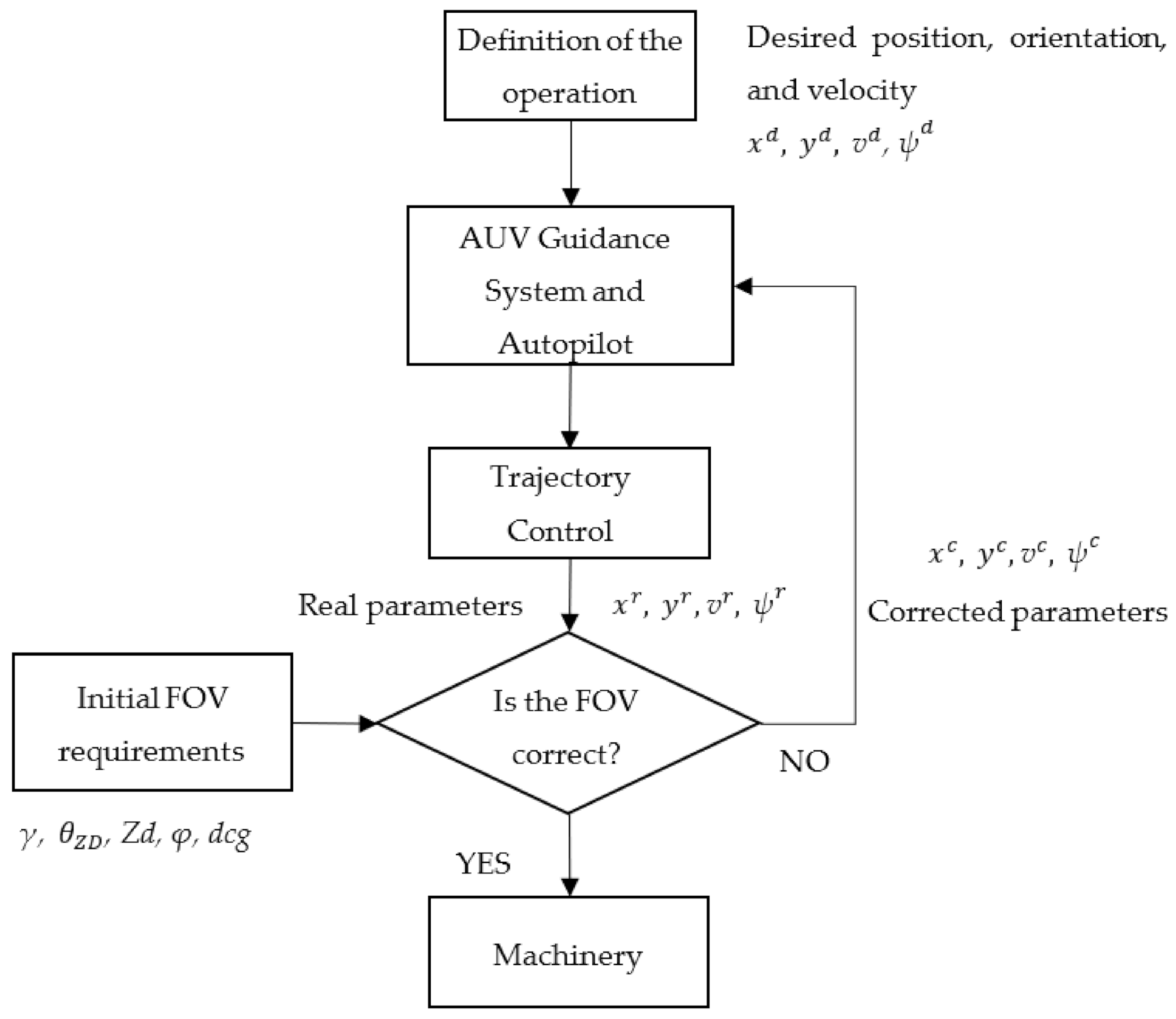
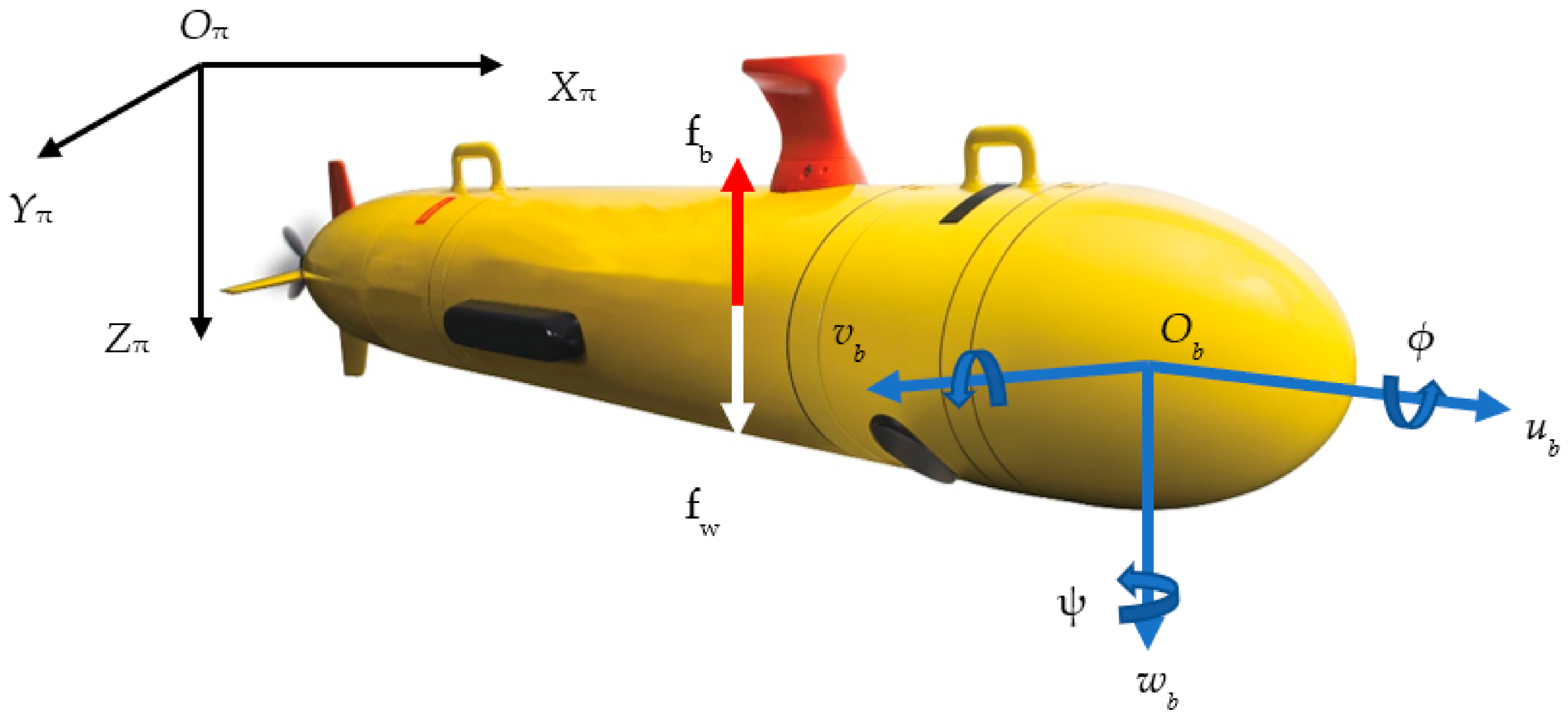
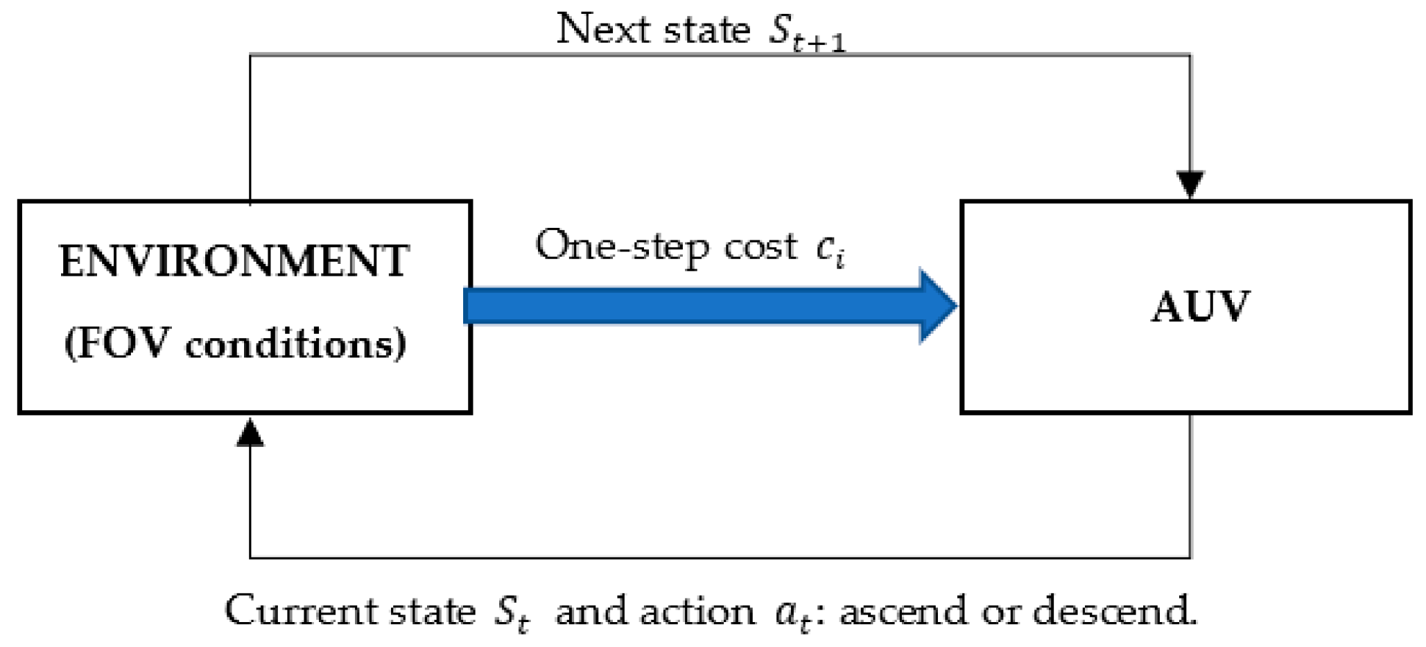
2.1. AUV Guidance System

The AUV receives information about the initial operational conditions which are combined in real time with the FOV requirements established by the operators. This model is applicable for any AUV type, control technique or navigation and mapping system. Several types of AUV are employed in underwater operations. Figure 4 shows the AUV body with the main variables for the navigation trajectory, being this type analysed in this paper.

AUV trajectory modelling considers hydromechanical aspects and the force system inherent in this type of vehicle. The dynamic motion equations of AUVs consider a body reference frame O_b and an inertial frame O_π, showed in Figure 4. This model also considers the hydrodynamic effects, generalized inertial forces, gravity, buoyancy, and force given by the thrusters. The dynamics of the vehicle can be studied according to the matrix equations proposed by Fossen [40], based on the general notation for submarine vehicles [18], and given by Equations (1) and (2):

$${M}\dot{\mathsf{\nu }}+C\left(\mathsf{\nu }\right)\mathsf{\nu }+D\left(\mathsf{\nu }\right)\mathsf{\nu } +g\left(\mathsf{\eta }\right)=\mathsf{\tau }$$

(1)

$$\dot{\mathsf{\eta }}=J\left(\mathsf{\eta }\right)\mathsf{\nu }$$

(2)

where M represents the inertial matrix; C(ν) are the terms of Coriolis; D(ν) is the hydrodynamic matrix; g(η) is the vector of hydrostatic forces; τ defines the vector of forces and moments in the body frame; J(η) is the kinematic transformation between the body and the inertial frame; η = [x, y, z, ϕ, θ, ψ] is the position of the vehicle and orientation in the inertial frame; and ν = [u, v, w] denotes the linear velocities in the body frame.

The model is simplified due to the complexity of the Equations (1) and (2). The AUV is determined with 6 degrees of freedom (DOFs), identifying the displacements, rotations and orientation [41]. The kinematic equations are given by Equations (3)–(5),

$$\dot{x_i} = u_i\cdot \cos \psi -{\upsilon }_i\cdot \sin \psi$$

(3)

$$\dot{y_i}= u_i\cdot \sin \psi +{\upsilon }_i\cdot \cos \psi$$

(4)

$$\dot{\psi } = w_i$$

(5)

where $x$ and $y$ are the coordinates of the centre of mass; $u$ and $\upsilon$ are the linear velocities of the AUV; $\psi$ the orientation, and $w$ describes the yaw velocity. The linear velocities are ($u,\upsilon ,w$), being the position and orientation ($x,y,\psi$).

The motion Equations (6)–(8) are defined avoiding the roll and the pitch motions,

$$\dot{u_i} = M_1\cdot \left(X_u\cdot u+a_{23}\cdot {\upsilon }_i\cdot w_i+{\tau }_u\right)$$

(6)

$$\dot{{\upsilon }_i} = M_2\cdot \left(Y_{\upsilon }\cdot {\upsilon }_i+a_{13}\cdot u_i\cdot w_i\right)$$

(7)

$$\dot{w} = M_3\cdot \left(N_i\cdot w_i+a_{12}\cdot u_i\cdot v_i + {\tau }_i\right)$$

(8)

where $X_u$, $Y_{\upsilon }$ and $N_i$ are the linear damping terms, and $M_1,$ $M_2,$ y, $M_3$ are terms related to the hydrodynamic mass and mass and inertia moment of the AUV. Coefficients $a_{23}$, $a_{13}$ and $a_{12}$ belong to the state variable associated with the dynamic equations.

Equation (8) shows the velocity in the yaw axis, which influences the characterization of the FOV. This will be defined in Section 2.2.

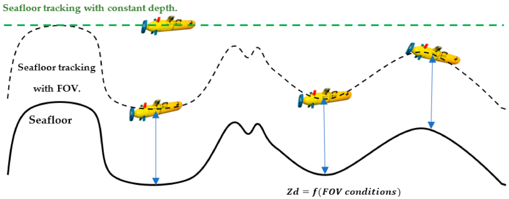
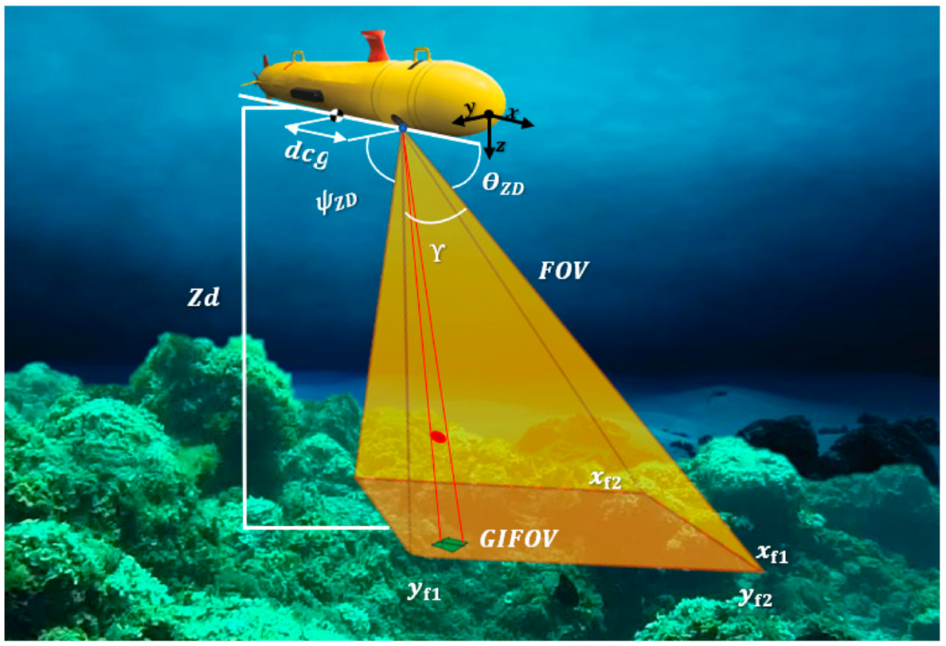
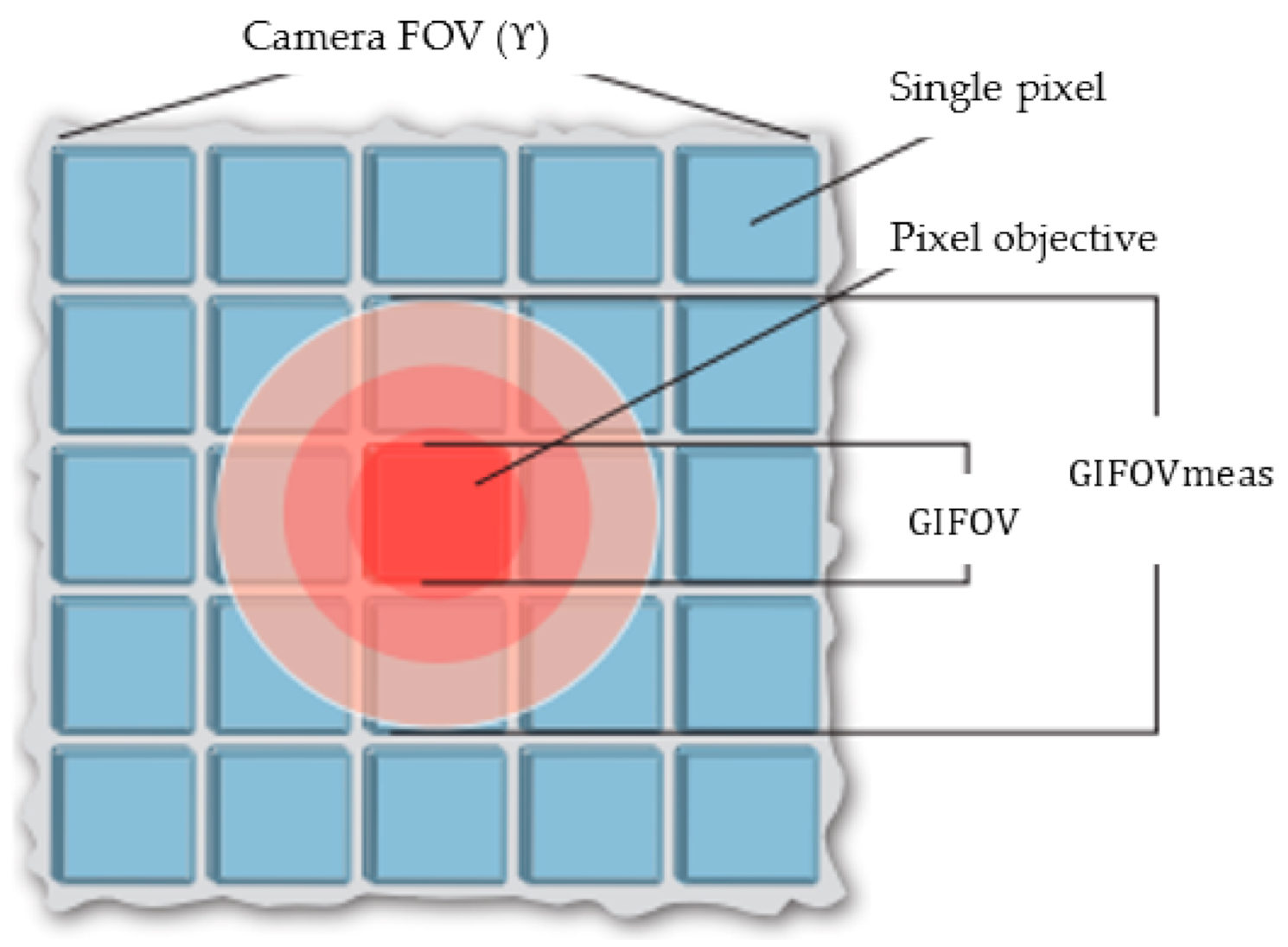
2.2. Determination of Underwater FOV

The operational trajectory is characterized automatically by selecting an area of interest, with the operator defining the conditions. The FOV determines the area covered by the camera or optical sensor according to trigonometric positioning. The initial FOV conditions are determined by the operator and limited by the environment, with the possibility of determining different ranges. The FOV of the operation is affected by the FOV defined in the specifications of the sensor or camera, environmental conditions and the AUV positioning and its trajectory. The main variables related to the operational FOV are: altitude (Zd) of the AUV from the seafloor; camera or sensor FOV (γ); camera or sensor payload inclination (${\theta }_{ZD}$); orientation of the sensor (${\psi }_{ZD}$); distance between sensor payload and centre of gravity (dcg), scattering, turbidity and absence of light [42]. The orientation of the sensor can be adapted to the requirements of the mission, being possible to set various orientations in the XZ and XY planes. The cameras or sonars are installed in fixed position or with self-stabilized mounting systems. The operator can control these values in real time or predefine certain actions. In the present study, the irregularity of the seafloor has not been considered, comprising part of the future work [43,44,45]. Figure 5 shows the main variables considered in the definition of the FOV.

The coordinates determined by the FOV of the operation are given by Equations (9)–(12) defined in reference [46].

$$x_{f1}=dcg+Z_d\cdot \tan \left(90-{\theta }_{ZD}-\frac{\gamma }{2}\right)$$

(9)

$$x_{f2}=dcg+ Z_d\cdot \tan \left({\theta }_{ZD}-\frac{\gamma }{2}\right)$$

(10)

$$y_{f1}=x_{f1}\cdot \tan \left({\psi }_{ZD}-\frac{\gamma }{2}\right)$$

(11)

$$y_{f2}=x_{f2}\cdot \tan \left({\psi }_{ZD}-90-\frac{\gamma }{2}\right)$$

(12)

where $x_{f1}$, $x_{f2}$ are the FOV positioning in the depth in the axis X, and $y_{f1}$, $y_{f2}$ are the FOV positioning in the depth in the axis Y.

The objective of any underwater operations is the maximization of the FOV, but an equilibrium between the increasing FOV is necessary together with ensuring a minimum reliable resolution to analyse the data. For this reason, the FOV is not enough for determining whether the measurement conditions provide suitable information or not. The Instantaneous FOV (IFOV) determines the capacity of the sensor/camera to detect details and is dependent on the technical requirement of the system [47]. The geometric resolution is represented in milliradians (mrad) and defines the smallest object in one pixel that can be represented in the image, depending on the measuring distance. This information is provided by the manufacturer of the monitoring system. The Ground IFOV (GIFOV) considers the single pixel size at ground level [48,49]. The type of the lens, measurement resolution of the camera and altitude modify the GIFOV. This value is measured in area unit per pixel in the case of cameras. It will be used as threshold for defining the reliability of the process according to the Equation (13).

$$\mathrm{GIFOV}=Zd\left|\tan ({\theta }_{ZD}-\frac{\mathrm{IFOV}}{2})-\tan (90-{\theta }_{ZD}-\frac{\mathrm{IFOV}}{2})\right|$$

(13)

The GIFOV value is theorical and it is not suitable for determining the reliability of the measurement process in real operations due to object reflect, distortions of optical systems or several issues in the acquisition systems. The measured GIFOV (GIFOVmeas) establishes the smallest detectable object in real conditions. The safety coefficient C is applied according to the requirements of the operation, being possible to choose different C values. C is a correction value that increments the GIFOV values ensuring proper measurements—see Equation (14).

$$\mathrm{GIFOVmeas}=\mathrm{GIFOV}\cdot C$$

(14)

References [46,50] propose C = 2 or C = 3 as suitable values. Higher C values increments the GIFOVmeas and the resolution of the images, ensuring a more suitable measurement process than reduced C values. For this reason, C = 3 is selected for this work. Figure 6 shows the comparison between the GIFOV and GIFOVmeas.

The GIFOVmeas is defined by the conditions of the operation. It will be used as decision factor in the analysis in real time of the operation, taking into account the minimum required resolution (R) and the AUV conditions according to Equation (15).

$$\mathrm{GIFOVmeas}<\mathrm{R}$$

(15)

As it was mentioned in previous sections, the adaptive trajectory modelling modifies the altitude conditions considering the FOV. In this case, Equations (13) and (14) is adapted in Equation (16) for this purpose, being $Z{d}_{FOV}$ the altitude depending on the FOV conditions and the GIFOVmeas defined by the operation requirements.

$$Z{d}_{FOV}=\frac{\mathrm{GIFOVmeas}}{\left|\tan ({\theta }_{ZD}-\frac{\mathrm{IFOV}}{2})-\tan (90-{\theta }_{ZD}-\frac{\mathrm{IFOV}}{2})\right|}$$

(16)

The relationship between the AUV motion and the FOV conditions is obtained by Equation (17) and by modifying Equation (8) to employ the FOV definition. The yaw velocity shows the variation of altitude per variation of time and, for this case study, the altitude is defined by the FOV conditions of the operation. Equation (17) combines motion equations and the relationship of the variations in the altitude in the FOV.

$$\dot{w}= M_3\cdot \left(N_i\cdot \frac{\Delta Z{d}_{FOV}}{\Delta t}+a_{12}\cdot u_i\cdot v_i + {\tau }_i\right)$$

(17)

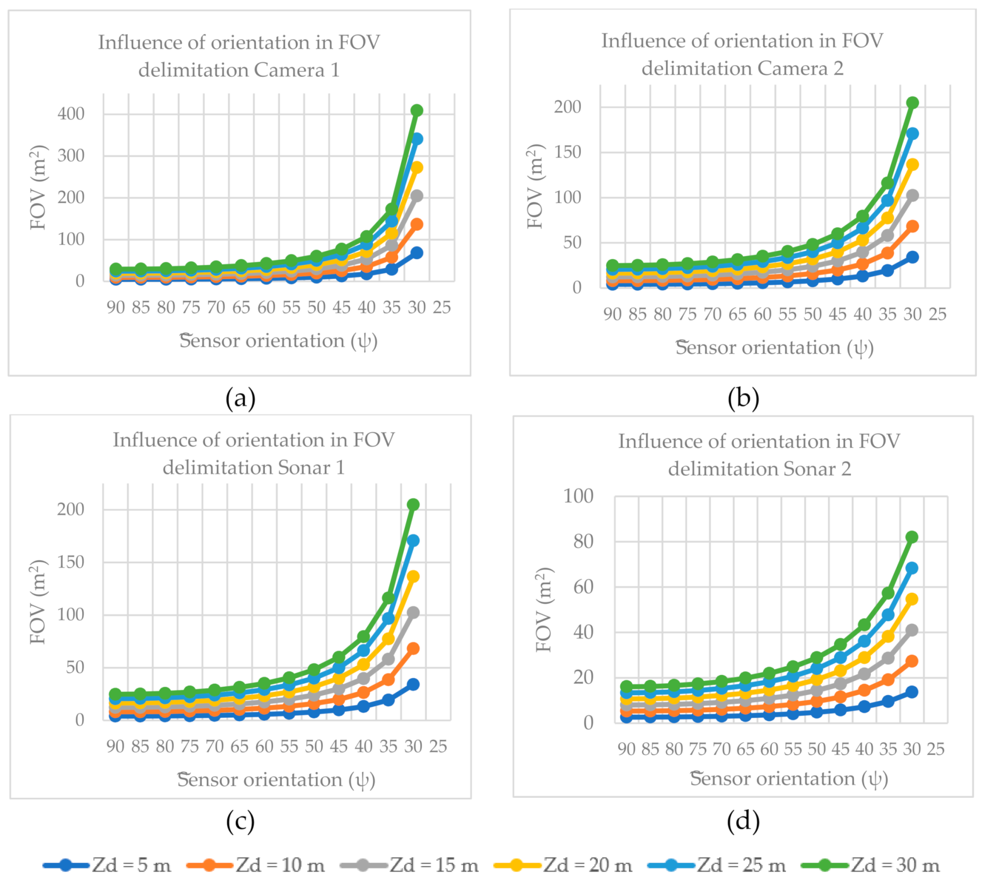
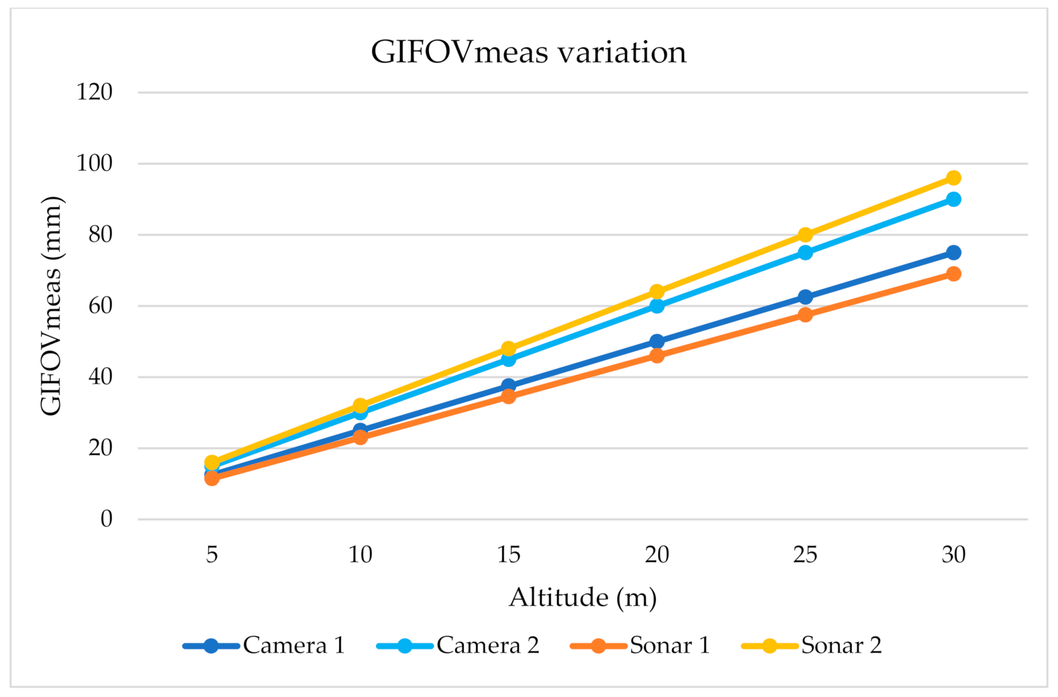
3. Case Studies and Results

In this section various commercial sonars and optical sensors are considered.

Table 1. Data acquisition characteristics summary. Data from [48,51].

Year	Data Acquisition System	Model	Ground Resolution (mm)	Sensor FOV (γ)
2014	Sonar 1	BlueViewP900-45 (Sonar)	2, 3	45°
2010	Camera 1	AVT Prosilica (Camera)	2, 5	52°
2014	Sonar 2	ARIS Explorer 3000 (Sonar)	3, 2	30°
2015	Camera 2	AVT Prosilica GC 1380 (Camera)	3	45°

summarises the information about different industrial sonars and cameras commonly used in underwater operations.

Figure 7 shows the FOV variations stablished with the Equations (9)–(12) for maintaining constant altitude from the seafloor for different inclinations of the camera or sonar. Different altitudes are proposed for analysing the increasing measured area.

The analysis of the results demonstrates the influence of the technical specifications of each system and the operational requirements in the data acquisition process. These results are used to identify certain combinations of altitude and inclination values for optimizing the measured area. An exponential trend with values greater than 50° in all data acquisition systems is observed, highlighting the increase in both sonars. The sensor orientations lower than 25° are discarded due to angles close to 0° can determine vertical measurement and inconsistent FOV values. The influence of the FOV of the sensors (γ) is critical since a difference of 7° between models causes an increase in the FOV of the operation by 200%—see Figure 7a,b. These results highlight the importance of the selection of the camera or sonar type. Despite the increase in the FOV with high values of inclination, a reliable measurement process is not ensured. Therefore, GIFOVmeas analysis is employed in each scenario. GIFOVmeas varies similarly with respect to sonar and camera, and it is used to validate the results—see Figure 8. These values are obtained by Equation (16) and are employed to set the operational thresholds as well as to determine the maximum depth according to the operation restrictions, the technical specifications of the AUV and the data acquisition system. The operators require a minimum resolution to ensure the further analysis of the data, and this information is compared with the GIFOVmeas determining the altitude of the operation. This information may be used to improve the path planning in the guidance system.

Once the GIFOVmeas is defined, it is possible to analyse the influence of the camera or sensor model in the $Zd$ definition. Using Equation (16) and for the case of camera 1, a $Zd$ value of 20 m is obtained when the operation requires a GIFOVmeas of 45 mm.

A scenario based on FOV analysis with traditional seafloor tracking at constant altitude and adaptive seafloor tracking considering the FOV conditions is proposed. A 2D model of the seafloor is introduced and adapted from reference [52]—see Figure 9.

The tracking modelling considering the FOV conditions is determined with the Markov decision process (MDP) for depth control. MDP is a stochastic process based on four phases: the state space, the action space, cost-function and transition probability [53]. MDP describes the state of the AUV and the actions to transit to the next state. For simplicity, it is only considered the depth control in the X-Z plane. For this case study, it is measured the relative depth and the actions determine if the AUV must ascend or descend regarding on the FOV conditions. Figure 10 shows the evolution of the MDP process: the initial state $S_t$ of the AUV develops an action $a_t$ used to change the next state $S_{t+1}$ according to the one-step cost $c_i$.

The state of the AUV, $S_t$, with adaptive trajectory considers the FOV conditions into the modelling process. Equation (18) shows the state of the AUV and it is designed to control the AUV tracking including the FOV requirements in the decision process. This process can be solved by several techniques, e.g., neural network or reinforced training, to obtain the next state of the AUV according to Wu et al. [53]. The altitude from the seafloor (Zd) is variable, being N the length of the curve, t denotes the time of the operation and FOV acquires all the conditions determined by the FOV of the operation.

$$\mathrm{AUV}state={\left[\Delta Z_D{ }_{\left(FOV, t-N+1\right)},\dots \Delta Z_D{ }_{\left(FOV, t-1\right)},\Delta Z_D{ }_{\left(FOV, t\right)}, \sin \theta , \cos \theta ,w_b,\theta , \dot{w}\right]}^T$$

(18)

For this scenario, devices shown in Table 1 with a sensor orientation of 45° are considered. The altitude has been determined in Figure 8 following the approach developed in the case of FOV consideration. This altitude is also applied for the constant depth modelling to compare both situations. The performance of each track mode is compared in Figure 11.

Figure 11a shows the altitude determined by each tracking model. The model with constant depth cannot modify the AUV trajectory regarding on the operational conditions and the performance of this model with changes in the altitude is limited. The AUV altitude takes into account the FOV conditions, and it implies a strong and stable response to changes in the seafloor shape. Equation 18 shows the current state of the AUV considering the parameters above described. If there is any variation, MDP processes the new conditions, where a time to identify the changing conditions of the seafloor is required to develop a suitable tracking behaviour to adapt it. The MDP issue has been solved following the methods defined in reference [53]. According to Wu et al. [53], the control process of the tracking considering the FOV produces a delay in the behaviour of the AUV causing a decrease in altitude and FOV when the seafloor shape presents the increasing slope, and an increase in both parameters when the seafloor shape is stabilized. The areas marked in red in Figure 11a,b show that the system needs time to adapt to the new conditions at 1000 and 2000 m. The C value defined for this scenario ensures variations in the FOV are within the limits, confirming a reliable measurement process despite the reduced FOV variations. Figure 11b shows the FOV results in both models for the devices shown in Table 1. The FOV with constant depth model increases because of the increase in the altitude. Sixty-two per cent of the measurement with this model is inaccurate, demonstrating the reliability of the model considering the FOV conditions.

4. Conclusions

Ocean floor surveys require new capabilities and techniques to overcome the endurance and operational limitations. Various technical issues and constraints may make very difficult the trajectory accuracy optimization in order to increase the quality of data obtained during the mission. The present paper presents a new methodology for optimizing the data acquisition process using AUVs. In current deep underwater operations, the FOV requirements of the data acquisition system are not included in the guidance system of the vehicles, limiting the reliability of the measurement process. The novelty proposed herewith considers the FOV in the trajectory development to increase the flexibility of these operations. The area of interest is determined considering the main parameters involved in the field of view. The vehicle trajectory is also defined considering the measurement process datasheets. A real case study, comparing different scenarios, is analysed to validate the results, highlighting the importance of the ground instantaneous field of view as decision factor in the submarine positioning. The present work also defines the basis of future work in the optimization of the underwater measurement process and sensor configuration.

References

1. Mayer, L.; Jakobsson, M.; Allen, G.; Dorschel, B.; Falconer, R.; Ferrini, V.; Lamarche, G.; Snaith, H.; Weatherall, P. The Nippon Foundation—GEBCO seabed 2030 project: The quest to see the world’s oceans completely mapped by 2030. Geosciences 2018, 8, 63. [Google Scholar] [CrossRef] [Green Version]
2. Wölfl, A.-C.; Snaith, H.; Amirebrahimi, S.; Devey, C.W.; Dorschel, B.; Ferrini, V.; Huvenne, V.A.; Jakobsson, M.; Jencks, J.; Johnston, G. Seafloor Mapping–the challenge of a truly global ocean bathymetry. Front. Mar. Sci. 2019, 6, 283. [Google Scholar] [CrossRef]
3. Jones, D.O.B.; Gates, A.R.; Huvenne, V.A.I.; Phillips, A.B.; Bett, B.J. Autonomous marine environmental monitoring: Application in decommissioned oil fields. Sci. Total Environ. 2019, 668, 835–853. [Google Scholar] [CrossRef]
4. Li, J.-H.; Park, D.; Ki, G. Autonomous swimming technology for an AUV operating in the underwater jacket structure environment. Int. J. Nav. Archit. Ocean Eng. 2019, 11, 679–687. [Google Scholar] [CrossRef]
5. Jung, M.-J.; Park, B.-C.; Bae, J.-H.; Shin, S.-H. PAUT-based defect detection method for submarine pressure hulls. Int. J. Nav. Archit. Ocean Eng. 2018, 10, 153–169. [Google Scholar] [CrossRef]
6. Jiang, Y.; Li, Y.; Su, Y.; Cao, J.; Li, Y.; Wang, Y.; Sun, Y. Statics variation analysis due to spatially moving of a full ocean depth autonomous underwater vehicle. Int. J. Nav. Archit. Ocean Eng. 2019, 11, 448–461. [Google Scholar] [CrossRef]
7. Gonen, B.; Akkaya, K.; Senel, F. Efficient camera selection for maximized target coverage in underwater acoustic sensor networks. In Proceedings of the 2015 IEEE 40th Conference onLocal Computer Networks (LCN), Clearwater Beach, FL, USA, 26–29 October 2015; pp. 470–473. [Google Scholar]
8. Huang, H.; Zhou, Z.; Li, H.; Zhou, H.; Xu, Y. The effects of the circulating water tunnel wall and support struts on hydrodynamic coefficients estimation for autonomous underwater vehicles. Int. J. Nav. Archit. Ocean Eng. 2020, 12, 1–10. [Google Scholar] [CrossRef]
9. Campos, E.; Monroy, J.; Abundis, H.; Chemori, A.; Creuze, V.; Torres, J. A nonlinear controller based on saturation functions with variable parameters to stabilize an AUV. Int. J. Nav. Archit. Ocean Eng. 2019, 11, 211–224. [Google Scholar] [CrossRef]
10. Gao, T.; Wang, Y.; Pang, Y.; Cao, J. Hull shape optimization for autonomous underwater vehicles using CFD. Eng. Appl. Comput. Fluid Mech. 2016, 10, 599–607. [Google Scholar] [CrossRef] [Green Version]
11. Sun, Y.-S.; Ran, X.-R.; Li, Y.-M.; Zhang, G.-C.; Zhang, Y.-H. Thruster fault diagnosis method based on Gaussian particle filter for autonomous underwater vehicles. Int. J. Nav. Archit. Ocean Eng. 2016, 8, 243–251. [Google Scholar] [CrossRef] [Green Version]
12. Belkin, I.; Sousa, J.B.d.; Pinto, J.; Mendes, R.; López-Castejón, F. Marine robotics exploration of a large-scale open-ocean front. In Proceedings of the 2018 IEEE/OES Autonomous Underwater Vehicle Workshop (AUV), Porto, Portugal, 6–9 November 2018; pp. 1–4. [Google Scholar]
13. Pliego Marugán, A.; Garcia Marquez, F.P.; Lev, B. Optimal decision-making via binary decision diagrams for investments under a risky environment. Int. J. Prod. Res. 2017, 55, 5271–5286. [Google Scholar] [CrossRef]
14. Marini, S.; Gjeci, N.; Govindaraj, S.; But, A.; Sportich, B.; Ottaviani, E.; Márquez, F.P.G.; Bernalte Sanchez, P.J.; Pedersen, J.; Clausen, C.V. ENDURUNS: An Integrated and Flexible Approach for Seabed Survey Through Autonomous Mobile Vehicles. J. Mar. Sci. Eng. 2020, 8, 633. [Google Scholar] [CrossRef]
15. Li, C.; Wang, P.; Li, T.; Dong, H. Performance study of a simplified shape optimization strategy for blended-wing-body underwater gliders. Int. J. Nav. Archit. Ocean Eng. 2020, 12, 455–467. [Google Scholar] [CrossRef]
16. Sánchez, P.J.B.; Papaelias, M.; Márquez, F.P.G. Autonomous underwater vehicles: Instrumentation and measurements. IEEE Instrum. Meas. Mag. 2020, 23, 105–114. [Google Scholar] [CrossRef]
17. Chen, H.-H.; Wang, C.-C.; Shiu, D.-C.; Lin, Y.-H. A preliminary study on positioning of an underwater vehicle based on feature matching of Seafloor Images. In Proceedings of the 2018 OCEANS-MTS/IEEE Kobe Techno-Oceans (OTO), Kobe, Japan, 28–31 May 2018; pp. 1–6. [Google Scholar]
18. Qiao, L.; Zhang, W. Adaptive non-singular integral terminal sliding mode tracking control for autonomous underwater vehicles. IET Control Theory Appl. 2017, 11, 1293–1306. [Google Scholar] [CrossRef]
19. Márquez, F.P.G. A new method for maintenance management employing principal component analysis. Struct. Durab. Health Monit. 2010, 6, 89. [Google Scholar]
20. Clarke, J.E.H. Multibeam echosounders. In Submarine Geomorphology; Springer: Berlin, Germany, 2018; pp. 25–41. [Google Scholar]
21. Herraiz, Á.H.; Marugán, A.P.; Márquez, F.P.G. Photovoltaic plant condition monitoring using thermal images analysis by convolutional neural network-based structure. Renew. Energy 2020, 153, 334–348. [Google Scholar] [CrossRef] [Green Version]
22. Noel, C.; Viala, C.; Marchetti, S.; Bauer, E.; Temmos, J. New tools for seabed monitoring using multi-sensors data fusion. In Quantitative Monitoring of the Underwater Environment; Springer: Berlin, Germany, 2016; pp. 25–30. [Google Scholar]
23. Segovia Ramírez, I.; Bernalte Sánchez, P.J.; Papaelias, M.; García Márquez, F.P. Autonomous underwater vehicles inspection management: Optimization of field of view and measurement process. In Proceedings of the 13th International Conference on Industrial Engineering and Industrial Management, Gijón, Spain, 11–12 July 2019. [Google Scholar]
24. Bobkov, V.A.; Mashentsev, V.Y.; Tolstonogov, A.Y.; Scherbatyuk, A.P. Adaptive method for AUV navigation using stereo vision. In Proceedings of the 26th International Ocean and Polar Engineering Conference, Rhodes, Greece, 26 June–2 July 2016. [Google Scholar]
25. Iscar, E.; Barbalata, C.; Goumas, N.; Johnson-Roberson, M. Towards low cost, deep water AUV optical mapping. In Proceedings of the OCEANS 2018 MTS/IEEE Charleston, Charleston, SC, USA, 22–25 October 2018; pp. 1–6. [Google Scholar]
26. Shea, D.; Dawe, D.; Dillon, J.; Chapman, S. Real-time SAS processing for high-arctic AUV surveys. In Proceedings of the 2014 IEEE/OES Autonomous Underwater Vehicles (AUV), Oxford, MS, USA, 6–9 October 2014; pp. 1–5. [Google Scholar]
27. Lucieer, V.L.; Forrest, A.L. Emerging Mapping Techniques for Autonomous Underwater Vehicles (AUVs). In Seafloor Mapping along Continental Shelves: Research and Techniques for Visualizing Benthic Environments; Finkl, C.W., Makowski, C., Eds.; Springer International Publishing: Cham, Switzerland, 2016; pp. 53–67. [Google Scholar] [CrossRef]
28. Hernández, J.; Istenič, K.; Gracias, N.; Palomeras, N.; Campos, R.; Vidal, E.; Garcia, R.; Carreras, M. Autonomous underwater navigation and optical mapping in unknown natural environments. Sensors 2016, 16, 1174. [Google Scholar] [CrossRef] [PubMed] [Green Version]
29. Braginsky, B.; Guterman, H. Obstacle avoidance approaches for autonomous underwater vehicle: Simulation and experimental results. IEEE J. Ocean. Eng. 2016, 41, 882–892. [Google Scholar] [CrossRef]
30. Hernández, J.D.; Vidal, E.; Moll, M.; Palomeras, N.; Carreras, M.; Kavraki, L.E. Online motion planning for unexplored underwater environments using autonomous underwater vehicles. J. Field Robot. 2019, 36, 370–396. [Google Scholar] [CrossRef]
31. Ramírez, I.S.; Marugán, A.P.; Márquez, F.P.G. Remotely Piloted Aircraft System and Engineering Management: A Real Case Study. In International Conference on Management Science and Engineering Management; Springer: Berlin, Germany, 2018; pp. 1173–1185. [Google Scholar]
32. Hou, W.; Gray, D.J.; Weidemann, A.D.; Fournier, G.R.; Forand, J. Automated underwater image restoration and retrieval of related optical properties. In Proceedings of the 2007 IEEE International Geoscience and Remote Sensing Symposium, Barcelona, Spain, 23–28 July 2007; pp. 1889–1892. [Google Scholar]
33. Jaffe, J.S. Underwater optical imaging: The past, the present, and the prospects. IEEE J. Ocean. Eng. 2014, 40, 683–700. [Google Scholar] [CrossRef]
34. Song, S.; Kim, B.; Yu, S.-C. Optical and acoustic image evaluation method for backtracking of AUV. In Proceedings of the OCEANS 2017-Anchorage, Anchorage, AK, 18–21 September 2017; pp. 1–6. [Google Scholar]
35. Lu, H.; Li, Y.; Nakashima, S.; Kim, H.; Serikawa, S. Underwater image super-resolution by descattering and fusion. IEEE Access 2017, 5, 670–679. [Google Scholar] [CrossRef]
36. Yau, T.; Gong, M.; Yang, Y.-H. Underwater camera calibration using wavelength triangulation. In Proceedings of the IEEE Conference on Computer Vision and Pattern Recognition, Portland, OR, USA, 23–28 June 2013; pp. 2499–2506. [Google Scholar]
37. Bhopale, P.; Bajaria, P.; Kazi, F.; Singh, N. LMI based depth control for autonomous underwater vehicle. In Proceedings of the 2016 International Conference on Control, Instrumentation, Communication and Computational Technologies (ICCICCT), Kumaracoil, India, 16–17 December 2016; pp. 477–481. [Google Scholar]
38. Li, J.-H.; Lee, P.-M. Design of an adaptive nonlinear controller for depth control of an autonomous underwater vehicle. Ocean Eng. 2005, 32, 2165–2181. [Google Scholar] [CrossRef]
39. Loc, M.B.; Choi, H.-S.; Seo, J.-M.; Baek, S.-H.; Kim, J.-Y. Development and control of a new AUV platform. Int. J. Control Autom. Syst. 2014, 12, 886–894. [Google Scholar] [CrossRef]
40. Fossen, T.I. Handbook of Marine Craft Hydrodynamics and Motion Control; John Wiley & Sons: Hoboken, NJ, USA, 2011. [Google Scholar]
41. Fossen, T.I. Marine Control Systems–Guidance. Navigation, and Control of Ships, Rigs and Underwater Vehicles. Marine Cybernetics, Trondheim, Norway, Org. Number NO 985 195 005 MVA, ISBN: 8292356002. Available online: www.marinecybernetics.com (accessed on 1 July 2020).
42. Gao, J.; Xu, D.; Zhao, N.; Yan, W. A potential field method for bottom navigation of autonomous underwater vehicles. In Proceedings of the 7th World Congress on Intelligent Control and Automation 2008 (WCICA 2008), Chongqing, China, 25–27 June 2008; pp. 7466–7470. [Google Scholar]
43. Smith Menandro, P.; Cardoso Bastos, A. Seabed Mapping: A Brief History from Meaningful Words. Geosciences 2020, 10, 273. [Google Scholar] [CrossRef]
44. Diesing, M.; Green, S.L.; Stephens, D.; Lark, R.M.; Stewart, H.A.; Dove, D. Mapping seabed sediments: Comparison of manual, geostatistical, object-based image analysis and machine learning approaches. Cont. Shelf Res. 2014, 84, 107–119. [Google Scholar] [CrossRef] [Green Version]
45. Elibol, A.; Gracias, N.; Garcia, R. Efficient Topology Estimation for Large Scale Optical Mapping; Springer: Berlin, Germany, 2012; Volume 82. [Google Scholar]
46. Segovia, I.; Pliego, A.; Papaelias, M.; Márquez, F.P.G. Optimal Management of Marine Inspection with Autonomous Underwater Vehicles; Springer: Berlin, Germany, 2019; pp. 760–771. [Google Scholar]
47. Márquez, F.P.G.; Ramírez, I.S. Condition monitoring system for solar power plants with radiometric and thermographic sensors embedded in unmanned aerial vehicles. Measurement 2019, 139, 152–162. [Google Scholar] [CrossRef] [Green Version]
48. Kwasnitschka, T.; Köser, K.; Sticklus, J.; Rothenbeck, M.; Weiß, T.; Wenzlaff, E.; Schoening, T.; Triebe, L.; Steinführer, A.; Devey, C.; et al. DeepSurveyCam—A Deep Ocean Optical Mapping System. Sensors 2016, 16, 164. [Google Scholar] [CrossRef] [Green Version]
49. Gonzalo, A.P.; Marugán, A.P.; Márquez, F.P.G. Survey of maintenance management for photovoltaic power systems. Renew. Sustain. Energy Rev. 2020, 134, 110347. [Google Scholar] [CrossRef]
50. McCamley, G.; Grant, I.; Jones, S.; Bellman, C. The impact of size variations in the ground instantaneous field of view of pixels on MODIS BRDF modelling. Int. J. Appl. Earth Obs. Geoinf. 2015, 38, 302–308. [Google Scholar] [CrossRef]
51. Hurtós Vilarnau, N. Forward-Looking Sonar Mosaicing for Underwater Environments. Doctoral Thesis, University of Girona Computer Architecture and Technology Department, Girona, Spain, 2014. [Google Scholar]
52. Li, Y.; Constable, S. 2D marine controlled-source electromagnetic modeling: Part 2—The effect of bathymetry. Geophysics 2007, 72, WA63–WA71. [Google Scholar] [CrossRef]
53. Wu, H.; Song, S.; You, K.; Wu, C. Depth control of model-free AUVs via reinforcement learning. IEEE Trans. Syst. ManCybern. Syst. 2018, 49, 2499–2510. [Google Scholar] [CrossRef] [Green Version]
Figure 1. Scheme of an Autonomous Underwater Vehicle (AUV).
Jmse 09 00277 g001
Figure 2. Seafloor tracking with Field of View (FOV) in comparison with traditional seafloor tracking.
Jmse 09 00277 g002
Figure 3. Diagram of the approach: AUV guidance system model including the FOV specifications.
Jmse 09 00277 g003
Figure 4. Coordinate frames in AUVs.
Jmse 09 00277 g004
Figure 5. AUV measurement conditions with FOV delimitation.
Jmse 09 00277 g005
Figure 6. GIFOVmeas definition.
Jmse 09 00277 g006
Figure 7. FOV variations for different depths and inclinations. Influence of orientation in FOV delimitation (a) Camera 1, (b) Camera 2, (c) Sonar 1 and (d) Sonar 2.
Jmse 09 00277 g007
Figure 8. Ground instantaneous FOV (GIFOV) variation in different cameras and sensors.
Jmse 09 00277 g008
Figure 9. Modelling of the seafloor.
Jmse 09 00277 g009
Figure 10. Evolution of MDP for depth tracking considering the FOV.
Jmse 09 00277 g010
Figure 11. (a) Altitude for both navigation models. (b) FOV for both navigation models.
Jmse 09 00277 g011aJmse 09 00277 g011b