LCTC Ships Concept Design in the North Europe- Mediterranean Transport Scenario Focusing on Intact Stability Issues

Abstract

In late years, the size of RoRo cargo ships has continuously increased, leading to the so-called Large Car Truck Carriers (LCTC). The design of these vessels introduced new challenges that shall be considered during the ship design since the conceptual stage, which has a very strong impact on the technical and economic performances of the vessel during all its life-cycle. In this work, the concept design of an LCTC is presented based on Multi-Attribute Decision Making (MADM). A large set of design alternatives have been generated and compared in order to find out the most promising feasible designs. The proposed approach is based on a Mathematical Design Model (MDM) capable to assess all the main technical and economic characteristics for each design. Among the others, here focus has been done on the ship stability to assure the compliance with statutory rules within the MDM. A new stability metamodel has been developed capable to define the cross curves of stability at the concept design stage. The proposed MADM methodology has been applied to North Europe-Mediterranean transport scenario highlighting the impact of main particulars describing hull geometry on the technical and economic performances of an LCTC ship.

1. Introduction

In the last decades, the global fleet of ships is significantly increasing in size and capacity. Considering the seaborne vehicle transport, standard Pure Car Truck Carriers (PCTC) have well-known limitation in draught, air draught and a conventional overall length below 200 m. However, in the very last years, some larger RoRo cargo vessels have been built. This new kind of vessel is usually referenced as Large Car Truck Carrier (LCTC) and represents a challenge for designers and operators. As all the innovative ship concepts, LCTC ships require an improvement in design methods to gain success in the global market. This need is true especially in the very initial design stage (concept design) since the most significant decisions are made there and can difficultly be enhanced in subsequent phases of the design process [1]. In fact, in the next design stages the freedom to make changes is reduced implying large waste of time and a huge increase of the design cost [2]. That requires permanent improvement in both analysis tools for performance prediction of feasible alternatives, and evaluation (decision making) techniques to form a balanced, flexible, and comprehensive design procedure [3].

Among the others decision-making techniques, the Multiple Attribute Decision-Making (MADM) offers a very effective tool to define and select the best possible design solution in the concept design stage. MADM has been already successfully applied on several types of vessel, including fishing vessels [4], fast ferries [5] and, more recently, bulk carriers [6], tankers [7] and Compressed Natural Gas (CNG) carriers [8]. Adopting MADM methods, all the technical and economical issues can be immediately addressed in order to assure the vessel feasibility and maximise the profit for the shipping company.

In this framework, a critical technical aspect is ship stability, since all the vessels shall comply with statutory regulations. Considering an LCTC, the stability problem shall be handled with particular care: too large values of the metacentric height $GM$ obviously comply with rules. However, it might drive to ship motions magnification in rough weather, leading also to severe cargo loss in the LCTC case. Therefore, at a conceptual stage, the design space is usually shifted towards a marginal compliance with stability rules. Hence, a reliable stability assessment procedure is already required during the concept design stage. Up to now, only a limited literature is available on this topic. A simple method for RoPax has been proposed by [9] based on the definition of $KG$ limit curve. A more complex approach as been proposed by [10] devoted to assess the righting arm curve of CNG ships.

Here, the stability issues within the overall concept design process are analysed for an LCTC vessel. A novel approach for the prediction of the cross curves of stability has been here studied introducing a quite large set of geometrical variables. Then, the resulting stability metamodel has been embedded in a Mathematical Design Model (MDM) part of a MADM framework. The proposed technique has been applied on the North Europe-Mediterranean transport scenario to select a tailored LCTC design. Moreover, in this specific geographical context, the link between the main hull geometry characteristics and the technical and economic performances of the ship is highlighted and discussed.

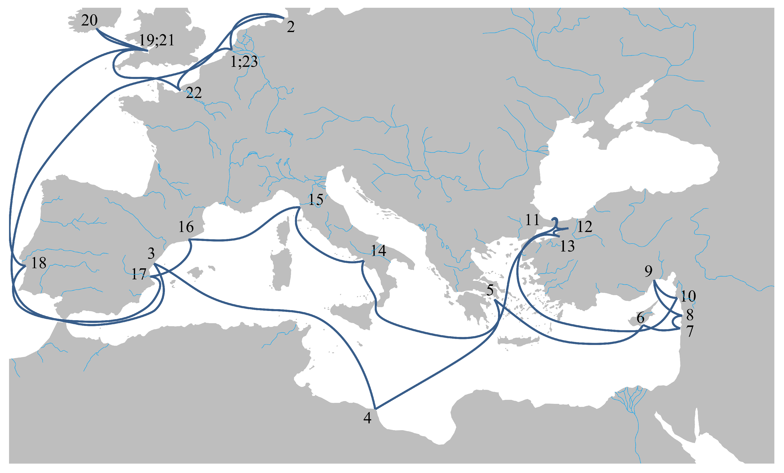
2. Transport Scenario

A typical Northern Europe-Mediterranean Sea route has been implemented to apply the MADM method for LCTC ships. The adopted route can be described as an inter-range route [11], despite no ocean has been crossed, because two sets of maritime ranges can be clearly identified, i.e., the ports next to the Channel and the ones in the Mediterranean Sea. The flow of vehicles also follows the same configuration as the route. In fact, there is one main flow in the North-South route, in which vehicles intended for different markets are transported. Besides, in short-range stops, most of (un)loading operations are due to the vehicles interchange for the local trade. However, in some main ports both the long- and short-range loading/unloading operations are present at the same time. Figure 1 depicts the modelled route, showing the stops in their consequential order. They are briefly described hereinafter.

Antwerp (1) has been chosen as starting port, being the ship loaded with almost one third of her total vehicles’s capacity. After a brief sail to Hamburg (2), where one more third of vehicles is loaded, the LCTC set sail to Sagunto (3), to take the rest of vehicles. Sagunto is the first stop in the Mediterranean Sea, where the ship mostly operates. After the unloading of one half of the vehicles in Misrata (4), the stop in Piraeus (5) port provides for the disembarkation of a small percentage of vehicles and the embarkation of a similar amount. From Piraeus, the ship stops in Limassol (6), Beirut (7), Tripoli (8), Mersin (9) and Lattakia (10), from which port sails up to Yenikoy (11) almost empty. In Autoport-Izmit (12) and Gemlik (13) the ship is loaded again and sails up to Salerno (14) at almost full load condition. In Livorno (15) and Barcelona (16) a more than one half of vehicles are discharged, while a small amount is loaded. Thus, in Valencia (17), the last Mediterranean stop, a significant percentage of vehicles can be loaded. In Setubal (18) there is a substantial equilibrium of loaded and unloaded vehicles. Then, the ship is involved in the short port-to-port [11] Portbury (19)-Cork (20)-Portbury (21). In Le Havre (22), all the vehicles loaded in Portbury are unloaded, before arriving to the last stops in Flushing and Antwerp (23), where the route ends and the ship is fully unloaded. Hence, a new cycle can start. Here the load factors have been taken independently from the ship scale.

Besides the loading/unloading rate, the modelled routing accounts for the dwell time at each port, the manoeuvre times in entering and leaving the ports, the rate of pilots and tugs. These expenditure items cannot be neglected for a reliable assessment of ship’s economic performances. Eventually, it has to be noticed that the ship never operates at the full-load condition. The average load condition along the considered route has been derived on the basis of actual information provided by a shipping company.

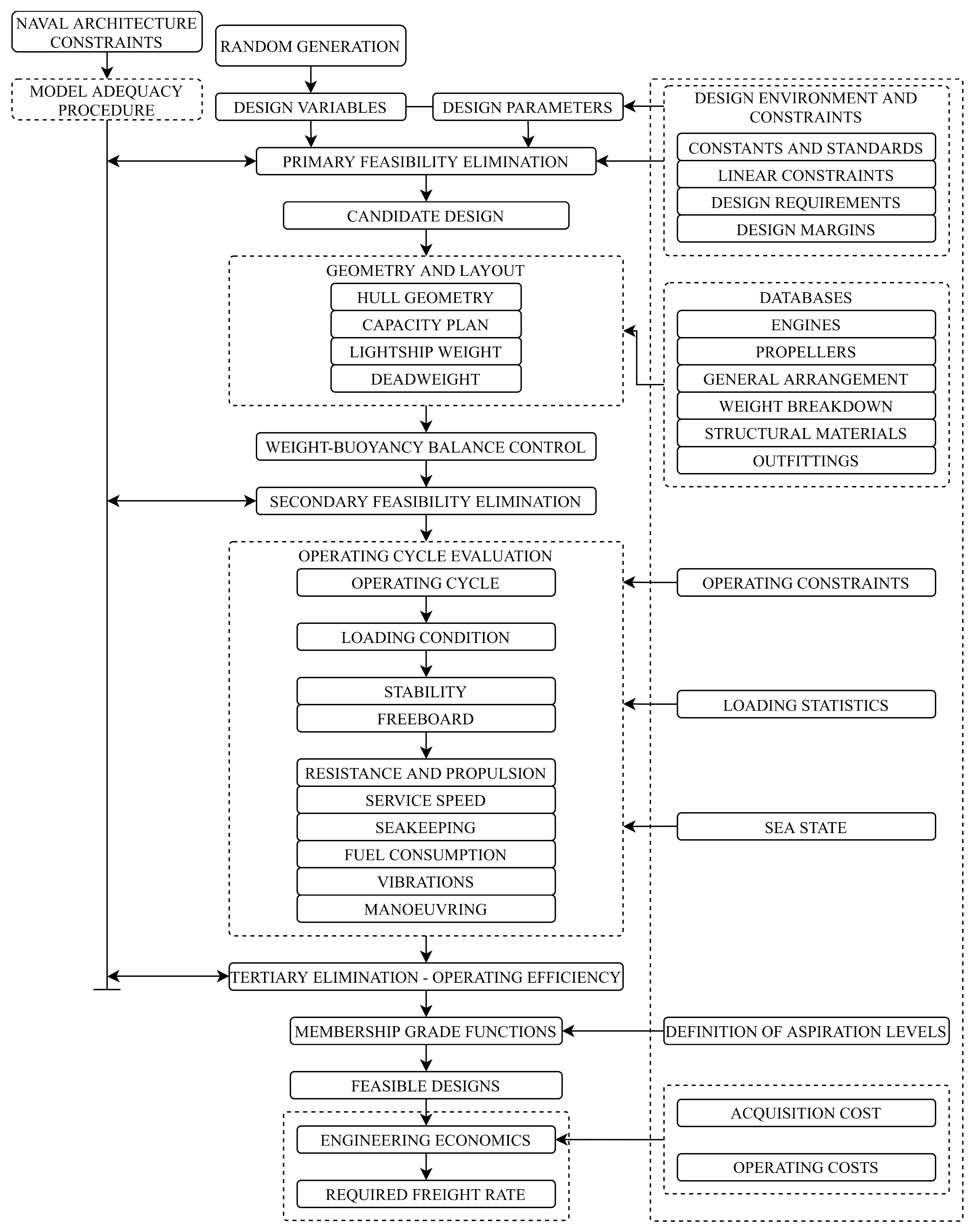
3. Concept Design Methodology

The complex, often conflicting, requirements in ship design can be simultaneously satisfied at concept design level using MADM techniques governed by multiple measures of performance of both technical and economic nature [12]. MADM techniques deal with generation and selection among a set of design alternatives described in terms of their properties (attributes) evaluated without any strict ordering, provided that concurrent engineering approach and analytic metamodels are introduced [13]. For instance, choosing and ranking among competitive ships described by simultaneous weighted attributes such as initial cost, size, main engine output, deadweight, and fuel economy is a typical multiple-attribute decision problem.

The MADM methodology is structured in an analysis model (the above-mentioned MDM) and a synthesis model (decision-making procedure), which identify the attribute space and the design space, respectively. The former generates and estimates the attributes of feasible designs, while the latter identifies the Pareto frontier of non-dominated designs, afterwards subject to some ranking technique [14].

3.1. Mathematical Design Model

Formulation of the MDM includes identification of the design variables (main dimensions and hull geometric coefficients), design parameters and design criteria (attributes and constraints). Parameters, such as lay-out of internal ramps, internal subdivision and stern ramp, are identical for all ships considered; this is also the case with a number of other outfit elements (e.g., stabilizers, superstructures, etc.). Constraints are functional and environmental requirements to prevent the design from attaining some unwanted characteristics. Constraints in the model basically belong to min-max, linear or non-linear type.

The MDM applied in the present work is summarised in Figure 2. It includes a set of analytic modules to estimate ship’s attributes in terms of the values of free variables and parameters, as well as an economic module to assess a merit index. Both the randomly generated hull characteristics (variables) and the evaluated attributes of each candidate ship are subject to constraint testing. A design not passing any constraint test is infeasible and eliminated from further evaluations. Among these constraints, stability rules play a key role on removing designs non-compliant with rule requirements. A detailed explanation of all the modules of MDM (Figure 2) goes beyond the purpose of the present paper, which focuses only on stability issues. Nevertheless, more details can be found in previous literature, such as [3,4,5,13,15,16,17,18].

Since the primary task of concept design is to find the ship size for required performance and payload as well as for the valuation of ship’s total cost, it is usual practice to include most of the ship linear dimensions and main coefficients in the set of free design variables of the MDM. Here, the design space is defined five design variables as reported in

Table 1. Free variables and applied ranges for the generation of LCTC design alternatives.

	L	B	T	${\mathit{C}}_{\mathit{P}}$	${\mathit{C}}_{\mathit{V}\mathit{P}}$
$min$	215.00	30.00	7.75	0.575	0.685
$max$	235.00	37.00	8.25	0.625	0.710

. Design variables are not completely free being subject to some constraints related to relations between them. Linear combination of the values of free variables and the ratios of free variables are the first constraints imposed after a set of variables is generated via Monte Carlo sampling. These constraints are needed in order to restrain the model from shifting to infeasible region of the design space.

Besides, the design parameters included in the MDM describe the basic configuration for all the candidate ships. Here, they include:

• hull form with transom stern and eight structural decks plus five hoistable car decks;
• single-screw propulsion system driven by a two-stroke diesel engine;
• accommodation and wheelhouse following IMO guidelines;
• single rudder and two bow-thrusters;
• stern loading only on the main deck with fixed ramp to weather deck and hoistable ramp to lower hold.

Attributes cover different qualities of the ship such as service speed, vertical acceleration, number of cars (payload), fuel consumption, building cost and economic merit index. Some of them, the so-called primary attributes, define the overall design quality, whilst others are used as constraints to check design feasibility. Here, the attributes given in

Table 2. Primary attributes in the design model.

Attribute	Description	Unit
$N_{car}$	Number of cars per cycle	(-)
$MDO$	Fuel consumption	(t/h)
$Powcf$	Power coefficient	(-)
$WB$	Ballast	(t)
${\ddot{\zeta }}_{wh}$	Vertical acceleration at the wheelhouse	($\mathrm{m}/{\mathrm{s}}^2$)
$I_t$	Turning index	(-)
$Capex$	Building cost	(mmUSD)
$Opex$	Operative cost	(mmUSD)
$RFR$	Required Freight Rate	(USD/car 1000 nm)

were selected as primary ones. All the attributes are assessed using several metamodels included in the present MDM for the LCTC ship, including hull form definition, net deck areas for cargo space, weight breakdown estimation, number of cars, powering at different service conditions, freeboard, intact and damage stability, seakeeping qualities, vibration levels, manoeuvering capabilities.

As regards ship vibrations, at concept design level it is deemed sufficient to control the main risk of resonance between vertical vibrations and propeller rate of revolutions by using the fuzzy set theory [19]. That is done by a membership grade function ${\mu }_{vib}$ [15] which activates the fuzzy control in order to avoid resonance with the first four natural frequencies of vertical hull vibrations and with the propeller blade frequency [5]. If $0.5\le {\mu }_{vib}<1$ (the larger the better) the ship is feasible, otherwise is discarded.

In order to properly account for technical and economic performances of the ship, an operative cycle should be defined. It should take care of the technological, economic and logistic environment, and is described by many items comprising required cycle time, loading/unloading time, manoeuvring time, covered distance at service speed, covered distance at reduced speed, time exposition to different sea states. The MDM includes a database containing information about environmental conditions along the service route in terms of annual-averaged probability of occurrence of significant wave heights and zero-cross periods. In order to offer a reliable transport system for scheduled arrival and departure times of ships, regardless of weather conditions and other unforeseeable circumstances, added resistance in waves and an allowance for shallow water have been introduced. Added resistance is assumed to manifest itself as reduced speed at constant fuel consumption, rather than the additional fuel consumption to maintain speed. Thus, over a typical voyage, the additional sea time is estimated and ships are discarded which do not comply with required scheduling. Once the propeller is selected through a sub-optimisation procedure in Sea State 4, the model selects the appropriate main engine under constrain that the continuous service rating is between 80–90%.

3.2. Engineering Economics

Harsh competition in the global market requires that several fundamental features and calculation methods should be anticipated at the level of concept design to improve the quality of the best possible designs. These include engineering economics, which is generally associated with the last phases of the basic design process. A reliable estimate of the building and operating costs of a new ship is one of the most difficult tasks of the design process. Moreover, in the concept design stage, it is hard to establish an accurate estimate of the costs, since the detail level is still too coarse. In fact, too many cost-dependent factors can be directly evaluated only after the completion of the embodiment design.

Experience gained by shipping operators has shown that ship’s overall life-cycle cost has become the primary decision criterion since early design phases [20]. Efficient economic evaluations are mandatory for the appropriate selection of the design variables values identifying the “best possible” solution in terms of both technical effectiveness and economic efficiency. There is extensive literature dedicated to the application of engineering economics in ship design, which started with the pioneering works of [21,22]. Various methods have been illustrated to make an economic estimate (average annual cost, discounted cash flows, etc.) and to suggest merit indexes (minimum required operating costs of the ship).

It is many decades since the significance of engineering economics in ship concept design has been recognized [18,23,24,25]. Here, all costs are evaluated in terms of the constant-value monetary unit. Cost-driven parameters have been compiled from operators’ data. Then, all cost-driven parameters have been directly correlated with design variables and parameters rather than introduced as averages, as it is still common practice in the shipbuilding companies.

Here, the required freight rate $RFR$ per unit carried serves as the main measure of merit to evaluate the economic merit of feasible designs [26]. $RFR$ is obtained by a sequential series of calculations in terms of discounted cash flows over the project life (N years) assuming a loan to be paid in equal instalments over r years to a compound interest rate i per annual payment period. Ship operating at the $RFR$ level would earn to the owner the same profit as if money was invested at the opportunity interest rate. $RFR$ is the preferred merit index where the annual payload is different between the various design alternatives. It implies that the “best possible” ship for the considered trade is the one that requires the lowest unit cost per nautical mile to the shipowner while returning to the customer the expected profit after taxes.

The required freight rate is evaluated as:

$$RFR=\sum _{i=0}^N\frac{AA{C}_i}{C_i}$$

(1)

where $ACC$ and C are the average annual cost and the annual transport capacity, respectively. Here, $AAC$ is the value obtained by imposing a zero net present value $NPV$ for each cash flow discounted to time zero, i.e., the time of signing the contract. The net present value is calculated as:

$$NPV=\sum _{i=0}^N{A}_i^{\prime }-\sum _{i=0}^{N}P{V}_{b_i}-\sum _{i=0}^{N}P{V}_{o_i}$$

(2)

where $A^{\prime }$ is the uniform annual return after taxes, including a 12% expected internal rate of return (IRR), related to the transported cars, and $P{V}_b$ and $P{V}_o$ are the present value of both investment (shipbuilding cost) and operating costs, respectively.

The estimate of building cost can be correlated to the ship’s weight components following the traditional approach based on ship work breakdown (SWBS) [27]. In the present work, data of ship’s cost components [28] have been updated according to confidential information from an Italian shipyard. Shipyard performance, productivity and construction methods have a direct influence on the absolute acquisition cost estimate. However, at concept design stage, systematic inaccuracies affect all the competing designs in a small amount, hence, their effect on the decision-making process is irrelevant. The building cost is divided into material costs, direct and indirect labour costs, miscellaneous costs (e.g., design fees, inspection costs, transport expenses) and overhead, which is taken as a fixed percentage of labour cost. Both material and labour costs account for hull steel, machinery and outfitting. The cost of steel construction varies almost linearly with steel weight. The cost per ton of outfitting is independent of size and is intended for a fixed seamen number. Miscellaneous costs are assessed as a function of lightship weight. The cost of main engines, including material, labour and overheads, is given as a function of engine power. The total cost of auxiliary machinery, including hull engineering, is assumed to be 2.5 times the cost of the main engine. Electric, electronic and auxiliary systems are given as input lump costs. Labour costs are based on man-hours, and once estimated, it is sufficient to apply wage rates, overhead and profit to assess them.

The operating costs are a function of several uncertain parameters, which are subject to the future trends on the global market. Hence, some assumptions are required in modelling the revenues and expenditures during the ship’s lifecycle. Hence, once again, the systematic inaccuracy or imprecision cannot heavily affect the ranking between the feasible ships. In ship-operation modelling, the primary variables are service speed and deadweight, which are strictly correlated to displacement and shaft horsepower. Other relevant variables are round-trip sea distance, operating days per year, port time along with fuel and lube oil consumption at sea and in port. Operating costs do not include the cost of lost time due to breakdown, since this is covered by the operation profile. In this work, the annual operating costs are broken down into manning and voyage costs. Voyage costs are all costs incurred by actual trips of the ship over a designated route and consist of costs of fuel oil and other consumables at sea and in port, cargo inventory costs, port charges and loading/unloading rates. The cost estimates for fuel and lube oil are based on the fuel consumption of the installed engines at the present spot fuel price. Manning costs consist of the annual running cost for maintenance and repairs, insurance, crew wages, provisions, stores and miscellaneous charges (e.g., administration and survey fees, recruiting and training crew, spare parts, ship services, personnel travel, catering and cleaning services).

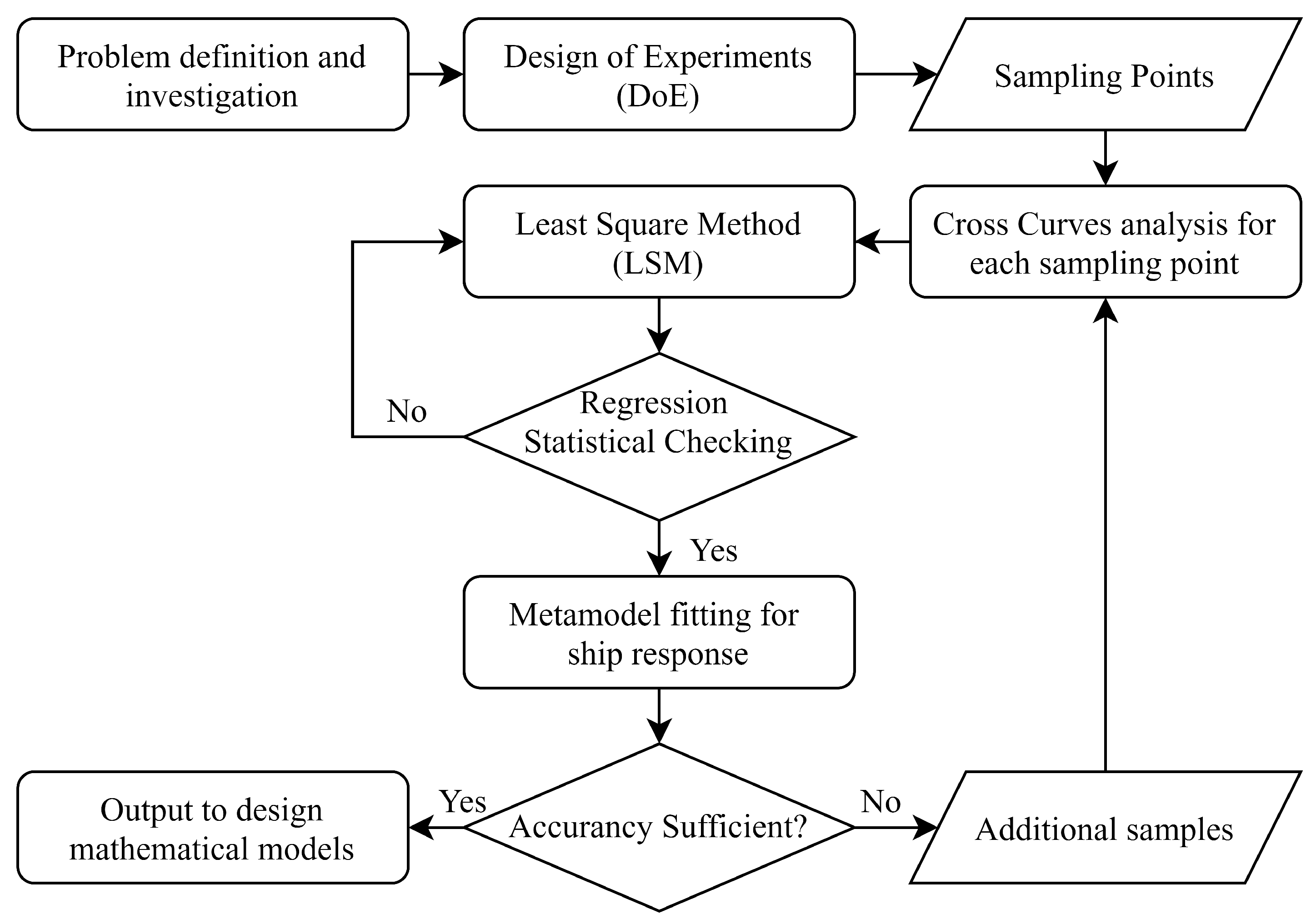
4. Stability Metamodel Methodology

In this section the methodology is presented to define a single metamodel part of the overall MDM. Here, the Multiple Linear Regression (MLR) method has been applied to define the stability metamodel, starting from a database of LCTC ships built with the Design of Experiment (DoE) method. With the proposed approach, the metacentric radius and the righting arm curve of a candidate ship can be predicted from its main geometrical parameters, without drawing the lines plan.

4.1. Variables Normalization

At the concept design stage, it is common practice to consider only non-dimensional variables describing the ship geometry in order to make them independent of the vessel size as far as possible. However, the variation range $[x_{min},x_{max}]$ of each variable can be considerably different in terms of absolute value inside the ship database. Hence, before applying the MLR method, the dependent and independent variables have been normalised in the range $[-1,1]$ to make them comparable and remove the effects connected to their different absolute values’ ranges. Considering a variable x, its normalised value $x^{\prime }$ can be evaluated as:

$$x^{\prime }=2\frac{x-x_{max}}{x_{max}-x_{min}}+1$$

(3)

This process shall be applied to both the independent and dependent variables. Then, on the results coming from the regression formulae, an inverse process has to be applied; that is, the normalized value of the estimated dependent variable $y^{\prime }$ has to be rescaled, according to:

$$y=y^{\prime }\frac{y_{max}-y_{min}}{2}+\frac{y_{max}+y_{min}}{2}$$

(4)

4.2. Multiple Linear Regressions

To build metamodels, the Multiple Linear Regression method has already been applied in the concept design phase with good results [10]. The MLR method provides an estimation of the response $y^{\prime }$ of a system as a function of n independent variables $x_i^{\prime }$. Here, since DoE has been adopted, a complete second-order surface response model can be used [29]. Hence, the dependent variable $y^{\prime }$ can be assessed as:

$$y^{\prime }=\sum _{i=0}^n\sum _{j=i}^n{C}_{ij}{x}_i^{\prime }{x}_j^{\prime }+\epsilon$$

(5)

where $x_0^{\prime }=1$, $C_{ij}$ are the unknown regression coefficients and $\epsilon$ is the regression error. Here, the least square method has been utilised to define the coefficients of the regression equation [30] as follows. First, the Equation (5) shall be rewritten in matrix form:

$$\mathbf{Y}=\mathbf{CX}+\epsilon$$

(6)

where $\mathbf{Y}$ contains the values of dependant variable, $\mathbf{X}$ is the matrix containing the related values of independent variables (each product $x_i^{\prime }{x}_j^{\prime }$ is considered one independent variable), $\mathbf{C}$ is the unknown coefficients vector and ${\mathit{\epsilon }}_{\mathit{r}}$ contains the regression errors. With such a notation, the regression coefficients are defined as:

$$\mathbf{C}={\left({\mathbf{X}}^T\mathbf{X}\right)}^{-1}{\mathbf{X}}^T\mathbf{Y}$$

(7)

The statistical adequacy of the regression equation has to be evaluated to assess the reliability of the results. This is done by measuring the error between estimated and observed values [29]. The adopted statistical indexes to check the regression strength are the sum of squared errors $SSE$, the determination coefficient $R^2$ and the adjusted determination coefficient $R_{adj}^2$. The $SSE$ is the sum of the squares of the difference between an observed value and the corresponding value estimated by the regression equation:

$$SSE=\sum _{i=1}^N{\left(y_i-y_i^{*}\right)}^2$$

(8)

where $y_i$ is the i-th observed value, $y_i^{*}$ is the i-th estimated value and N is the number of data points, i.e., the number of ships within the database. The determination coefficient $R^2$ is a statistical index that represents the proportion of the variance of the dependent variable from the independent variables that are used for its estimation:

$$R^2=1-\frac{SSE}{S{S}_{tot}}$$

(9)

where $S{S}_{tot}$ is the corrected total Sum of Squares evaluated as:

$$S{S}_{tot}=\sum _{i=1}^N{\left(y_i-\overline{y}\right)}^2$$

(10)

being $\overline{y}$ the mean value. The adjusted determination coefficient $R_{adj}^2$ is evaluated as:

$$R_{adj}^2=1-\left(1-R^2\right)\frac{N-1}{N-p-1}$$

(11)

where p denotes the number of explanatory terms (i.e., the relevant independent variables). The $R_{adj}^2$ index is preferable, as it is independent of the number of explanatory terms.

Since only certain variables influence the response, a selection is required. Among the methods available in literature, the relevant variables selection has been carried out applying the stepwise selection process [31], which systematically adds and removes variables on the base of their statistical significance. Here the $R_{adj}^2$ is used, assuming entrance and exit tolerances equal to 0.01 and 0.00001, respectively. Besides, also variables’ p-values have been considered in the removal process, excluding all the variables having a p-value greater than 0.05.

4.3. Proposed Formulation

The main objective of the stability metamodel is to ensure that an alternative design fulfils the stability regulations. That is why, within the MDM, compliance with IMO rules is considered a crisp constraint to remove unfeasible designs. Considering a LCTC, the issues related to damage stability are limited to the number of bulkheads in the double hull as well as the value of the inner hull distance from the external hull. Therefore, damage stability is addressed in the structural metamodel, while here special attention is given to the intact stability problem. As most cargo vessels, LCTC ships have to comply with the intact stability code [32], which impose requirements on the metacentric height (initial stability), the righting lever shape and the ship behaviour in a severe seaway. Hence, in order to check the compliance with rule requirements, the metacentric height $GM$ and the righting arm curve $GZ$ have to be evaluated.

In previous studies, the $GZ$ curve has been directly evaluated through one or more regression equations including the $KG/T$ as an independent variable [10]. However, this approach encompasses both geometrical aspects (the shape of the cross curves of stability) and mechanical aspects (related to the lightship weight and loading condition). To decouple the two problems, a new stability metamodel has been developed to predict the cross curves of stability $KN=f\left(\phi \right)$ of an LCTC from its main geometrical particulars. Then, the $GZ$ curve can be assessed for multiple loading conditions evaluated on the basis of the capacity plan, lightship weight and deadweight metamodels, providing the actual $KG$:

$$GZ\left(\phi \right)=KN\left(\phi \right)-KGsin\left(\phi \right)$$

(12)

The process adopted to define the intact stability metamodel is schematically shown in Figure 3. For each ship within the database (sampling point) the cross curve of stability has been evaluated. The $KN$ has been obtained for angles of heel ranging between 0 deg and 60 deg every 5 deg. Then, the non-dimensional coefficient $KN/B$ has been calculated and normalised in the $[-1,1]$ range. A specific regression has been obtained applying the MLR methodology for each angle of heel in the form:

$${\left(\frac{KN}{B}\right)}^{\prime }\left({\phi }_k\right)=C_{0,0}+\sum _{i=1}^7{C}_{0,i}\left({\phi }_k\right)x_i^{\prime }+\sum _{i=1}^7\sum _{j=i+1}^7{C}_{ij}\left({\phi }_k\right)x_i^{\prime }{x}_j^{\prime }+\sum _{i=1}^7{C}_{i,i}\left({\phi }_k\right){x_i^{\prime }}^2$$

(13)

The independent variables adopted to define the regressions on cross curves of stability toghether with there extreme values are summarised in

Table 3. Primitive variables for stability.

Independent Variable Short Name	$\mathit{L}/\mathit{B}$ ${\mathit{x}}_1$	$\mathit{B}/\mathit{T}$ ${\mathit{x}}_2$	${\mathit{C}}_{\mathit{X}}$ ${\mathit{x}}_3$	${\mathit{C}}_{\mathit{P}}$ ${\mathit{x}}_4$	${\mathit{C}}_{\mathit{W}\mathit{P}}$ ${\mathit{x}}_5$	$\mathit{T}/\mathit{D}$ ${\mathit{x}}_6$	${\mathit{C}}_{\mathit{V}\mathit{P}}$ ${\mathit{x}}_7$
$x_{min}$	4.689	3.793	0.900	0.532	0.815	0.339	0.613
$x_{max}$	6.811	5.207	0.980	0.851	0.960	0.500	0.839

. This set has been considered sufficient to completely define the stability problem and to present a large range of variation within the ships’ database. Besides, the initial stability shall be also considered in order to check the requirements on $GM$ according to rules [32]. Again the $GM$ is evaluated decoupling geometric and mechanical components as:

$$GM=KM-KG$$

(14)

The $KM$ is again obtained applying the MLR method as:

$${\left(\frac{KM}{B}\right)}^{\prime }=C_{0,0}+\sum _{i=1}^7{C}_{0,i}{x}_i^{\prime }+\sum _{i=1}^7\sum _{j=i+1}^7{C}_{ij}{x}_i^{\prime }{x}_j^{\prime }+\sum _{i=1}^7{C}_{i,i}{x_i^{\prime }}^2$$

(15)

It is worth noting that independent variables set adopted in the stability metamodel differs from the design variables set randomly generated in the MDM. This is due to the peculiarities of stability problem. Within the MDM other statistical formulae are adopted within the hull geometry metamodel to estimate all the geometric parameters from the design variables.

5. Application

In the present section the application of the proposed methodology to define a stability metamodel is presented, addressing the issues related to the intact stability of an LCTC. Since only a limited number of LCTCs are currently in operation, a larger database of mathematically-defined hull forms of LCTCs has been built to perform statistical analysis. Then, the obtained regression coefficients are presented and discussed along with the validation of the metamodel over two hull forms not included in the design database.

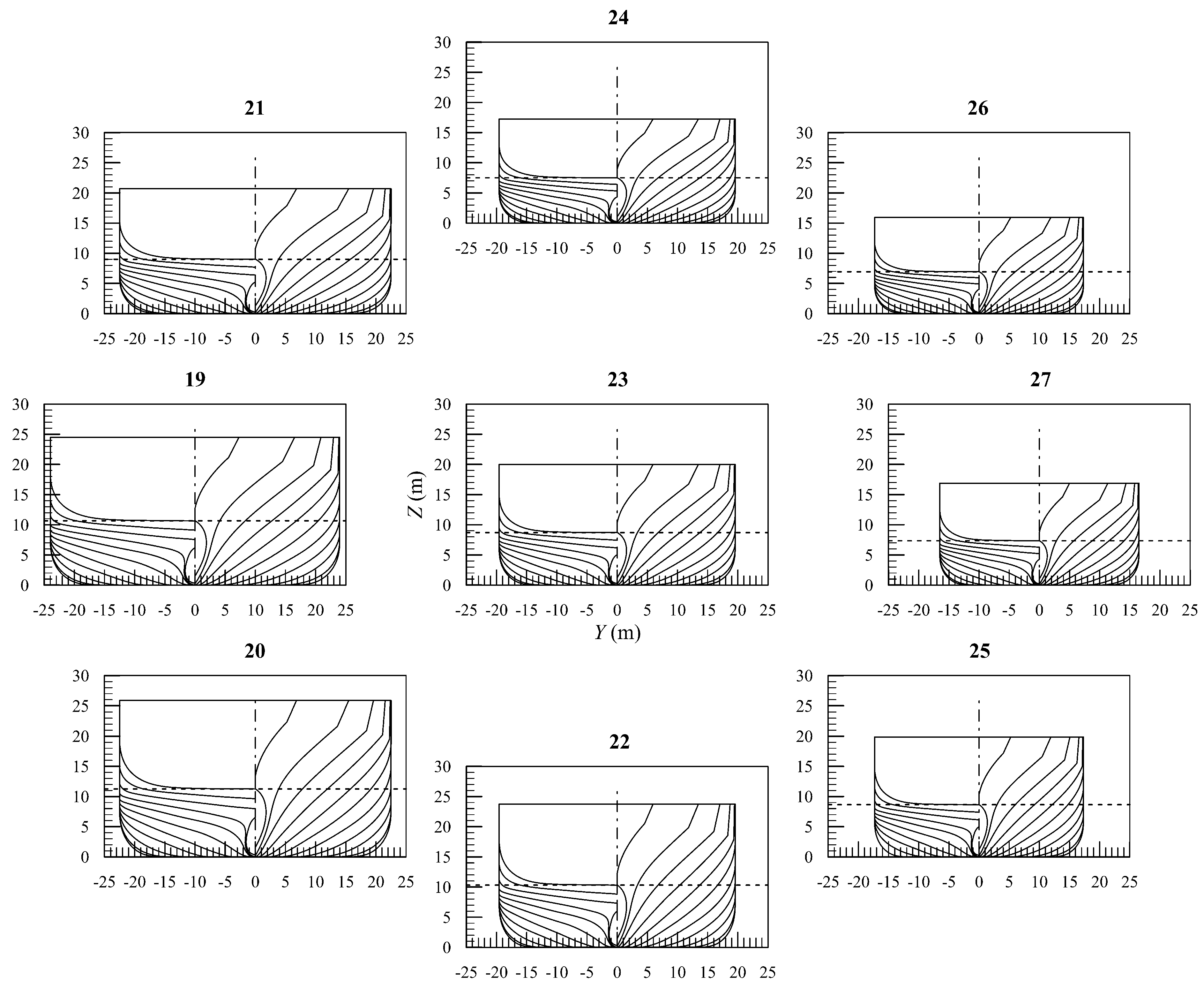
5.1. Database Generation

As mentioned, the metamodels are usually based on the results of statistical analysis performed on a database of ships. In the engineering field, when data are lacking or it is necessary to explore a new design space it is common practice to generate a proper database fitting the design team requirements. In order to limit the number of ships within the database, the design of experiments (DoE) can be applied to cover a predefined range of a set of independent variables [33]. However, due to the LCTC peculiarities, the database has not been generated by a straightforward application of DoE, since it might lead to unfeasible hull forms from the propulsion or structural point of view. Here, a two-step approach has been applied: first, several parent hulls have been defined, and then they have been scaled to cover all the design space.

Usually, when DoE is applied, a set of variations is defined starting from a parent hull. Each variation is obtained by scaling the parent geometry and modifying the block coefficient $C_B$ and the longitudinal position of the centre of buoyancy $LCB$ using the Lackenby method. This approach generates hull geometries that are strictly related to the parent hull. In detail, the midship section coefficient $C_X$ cannot be changed, bounding the value of the prismatic coefficient $C_P$, too. To investigate different combinations of $C_X$ and $C_P$, here, nine parent hulls have been defined having constant $L/B$ and $B/T$ ratios and length ranging from 190 m to 225 m. The parent hulls’ coefficients ($C_P$ and $C_X$) have been defined according to the Central Composite Circumscribed Design [34], as reported in

Table 4. Primary geometrical characteristics of parent hulls.

L [m]	$\mathit{L}/\mathit{B}$	$\mathit{B}/\mathit{T}$	${\mathit{C}}_{\mathit{X}}$	${\mathit{C}}_{\mathit{B}}$
190	5.750	4.500	0.940	0.650
200	5.750	4.500	0.940	0.800
205	5.750	4.500	0.940	0.500
210	5.750	4.500	0.980	0.650
215	5.750	4.500	0.900	0.650
220	5.750	4.500	0.968	0.756
225	5.750	4.500	0.968	0.544
195	5.750	4.500	0.912	0.756

. All the parent hulls share some common features, i.e., bulbous bow, single screw stern bulb, dry transom. The parent hull forms have been optimised for their specific value $C_X$ and $C_P$ applying a proper $LCB$ and half entrance angle chosen according to preliminary estimation of hull resistance and propulsion. These assumptions affect the waterplane area, driving to the cumulative distributions of $C_{WP}$ and $C_{VP}$ provided in Figure 4a,b, which result to be almost uniformly distributed within the database.

Then, for each parent hull, the Central Composite Circumscribed Design has been again applied to generate a sub-family of ships having the same length and different $L/B$ and $B/T$ ratios. As an example, Figure 5 shows the body plans of the hulls having $C_X=0.968$ and $C_P=0.562$. The final database consists of $N=72$ ships having the characteristics summarised in

Table 5. Main particulars of the ships within the database.

ID	$\mathit{L}/\mathit{B}$	$\mathit{B}/\mathit{T}$	${\mathit{C}}_{\mathit{X}}$	${\mathit{C}}_{\mathit{P}}$	${\mathit{C}}_{\mathit{W}\mathit{P}}$	$\mathit{T}/\mathit{D}$	${\mathit{C}}_{\mathit{V}\mathit{P}}$	ID	$\mathit{L}/\mathit{B}$	$\mathit{B}/\mathit{T}$	${\mathit{C}}_{\mathit{X}}$	${\mathit{C}}_{\mathit{P}}$	${\mathit{C}}_{\mathit{W}\mathit{P}}$	$\mathit{T}/\mathit{D}$	${\mathit{C}}_{\mathit{V}\mathit{P}}$
1	4.689	4.500	0.940	0.691	0.842	0.457	0.772	37	4.689	4.500	0.940	0.532	0.815	0.470	0.613
2	5.000	4.000	0.940	0.691	0.843	0.471	0.771	38	5.000	4.000	0.940	0.532	0.815	0.484	0.613
3	5.000	5.000	0.940	0.691	0.843	0.416	0.771	39	5.000	5.000	0.940	0.532	0.815	0.429	0.613
4	5.750	3.793	0.940	0.691	0.842	0.449	0.772	40	5.750	3.793	0.940	0.532	0.815	0.462	0.613
5	5.750	4.500	0.940	0.691	0.842	0.407	0.772	41	5.750	4.500	0.940	0.532	0.815	0.420	0.613
6	5.750	5.207	0.940	0.691	0.842	0.368	0.772	42	5.750	5.207	0.940	0.532	0.815	0.385	0.613
7	6.500	4.000	0.940	0.691	0.842	0.406	0.772	43	6.500	4.000	0.940	0.532	0.815	0.419	0.613
8	6.500	5.000	0.940	0.691	0.842	0.339	0.772	44	6.500	5.000	0.940	0.532	0.815	0.366	0.613
9	6.811	4.500	0.940	0.691	0.842	0.360	0.772	45	6.811	4.500	0.940	0.532	0.815	0.380	0.613
10	4.689	4.500	0.900	0.722	0.897	0.479	0.724	46	4.689	4.500	0.940	0.851	0.960	0.466	0.834
11	5.000	4.000	0.900	0.722	0.898	0.492	0.723	47	5.000	4.000	0.940	0.851	0.960	0.480	0.834
12	5.000	5.000	0.900	0.722	0.899	0.437	0.723	48	5.000	5.000	0.940	0.851	0.960	0.424	0.834
13	5.750	3.793	0.900	0.722	0.898	0.471	0.724	49	5.750	3.793	0.940	0.851	0.960	0.458	0.834
14	5.750	4.500	0.900	0.722	0.898	0.428	0.724	50	5.750	4.500	0.940	0.851	0.960	0.416	0.834
15	5.750	5.207	0.900	0.722	0.898	0.393	0.724	51	5.750	5.207	0.940	0.851	0.960	0.381	0.834
16	6.500	4.000	0.900	0.722	0.899	0.427	0.723	52	6.500	4.000	0.940	0.851	0.960	0.415	0.834
17	6.500	5.000	0.900	0.722	0.899	0.374	0.723	53	6.500	5.000	0.940	0.851	0.960	0.357	0.833
18	6.811	4.500	0.900	0.722	0.898	0.387	0.724	54	6.811	4.500	0.940	0.851	0.959	0.376	0.834
19	4.689	4.500	0.968	0.562	0.831	0.487	0.654	55	4.689	4.500	0.980	0.663	0.863	0.475	0.753
20	5.000	4.000	0.968	0.562	0.831	0.500	0.655	56	5.000	4.000	0.980	0.663	0.863	0.488	0.753
21	5.000	5.000	0.968	0.562	0.831	0.445	0.655	57	5.000	5.000	0.980	0.663	0.863	0.433	0.754
22	5.750	3.793	0.968	0.562	0.831	0.478	0.655	58	5.750	3.793	0.980	0.663	0.862	0.466	0.754
23	5.750	4.500	0.968	0.562	0.830	0.436	0.655	59	5.750	4.500	0.980	0.663	0.863	0.424	0.754
24	5.750	5.207	0.968	0.562	0.832	0.401	0.654	60	5.750	5.207	0.980	0.663	0.862	0.389	0.754
25	6.500	4.000	0.968	0.562	0.832	0.435	0.654	61	6.500	4.000	0.980	0.663	0.863	0.423	0.754
26	6.500	5.000	0.968	0.562	0.830	0.381	0.655	62	6.500	5.000	0.980	0.663	0.862	0.370	0.754
27	6.811	4.500	0.968	0.562	0.830	0.395	0.655	63	6.811	4.500	0.980	0.663	0.863	0.383	0.753
28	4.689	4.500	0.968	0.781	0.902	0.484	0.838	64	4.689	4.500	0.912	0.829	0.946	0.462	0.799
29	5.000	4.000	0.968	0.781	0.901	0.497	0.839	65	5.000	4.000	0.912	0.829	0.946	0.475	0.799
30	5.000	5.000	0.968	0.781	0.902	0.442	0.839	66	5.000	5.000	0.912	0.829	0.945	0.420	0.800
31	5.750	3.793	0.968	0.781	0.902	0.476	0.839	67	5.750	3.793	0.912	0.829	0.947	0.454	0.798
32	5.750	4.500	0.968	0.781	0.901	0.433	0.839	68	5.750	4.500	0.912	0.829	0.946	0.412	0.799
33	5.750	5.207	0.968	0.781	0.902	0.398	0.839	69	5.750	5.207	0.912	0.829	0.945	0.377	0.800
34	6.500	4.000	0.968	0.781	0.902	0.432	0.838	70	6.500	4.000	0.912	0.829	0.947	0.410	0.798
35	6.500	5.000	0.968	0.781	0.902	0.378	0.838	71	6.500	5.000	0.912	0.829	0.946	0.348	0.799
36	6.811	4.500	0.968	0.781	0.902	0.392	0.838	72	6.811	4.500	0.912	0.829	0.946	0.369	0.799

. The ranges of the ship geometric parameters in the database have been chosen according to an analysis of the existing fleet of LCTC ship operating worldwide.

Aiming at putting ship stability under strict control, the depth moulded (D) measured at the freeboard deck is a key parameter, since it has a strong effect on the righting arm curve shape. Considering LCTC vessels, the depth is mainly subject to constraints related to cargo (deck height) and structural issues (beams height, double bottom height). Hence, for each ship in the database, a proper value of D has been defined according to a preliminary midship section layout. Then, the non-dimensional $T/D$ ratio has been evaluated (Table 5). It is worth noting that the resulting $T/D$ distribution is almost uniform within the database population. In Figure 4c the $T/D$ Cumulative Density Function (CDF) pattern is shown.

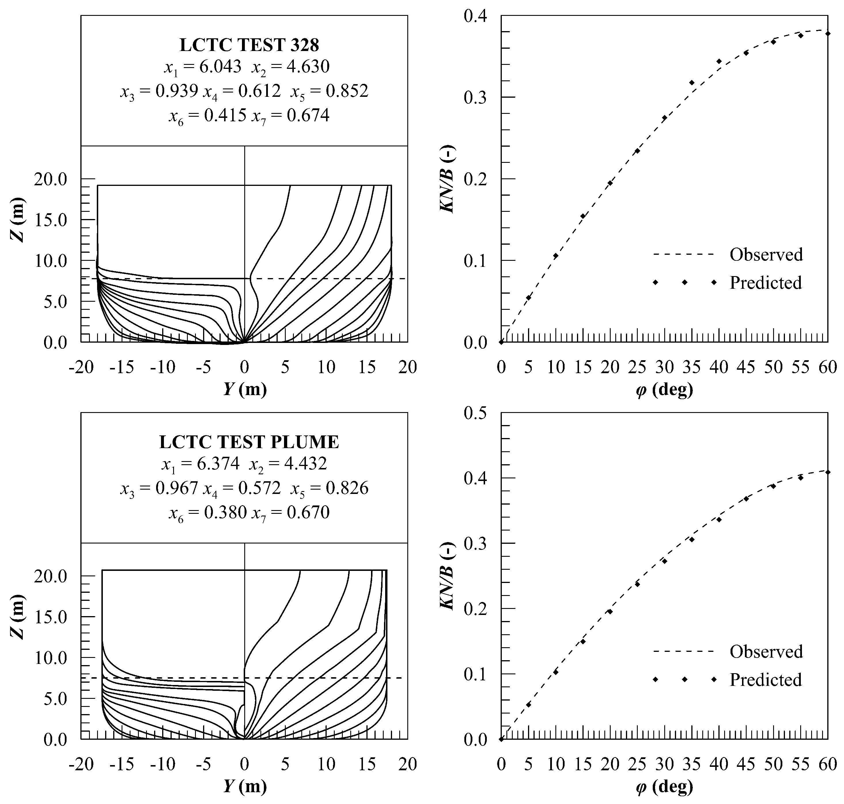
5.2. Ship Stability Prediction

Applying the proposed methodology, the regression coefficients for the stability metamodel have been determined. The results are provided in

Table 6. Regression coefficients for the stability metamodel.

	${\left(\frac{\mathit{K}\mathit{N}}{\mathit{B}}\right)}^{\prime }$												${\left(\frac{\mathit{K}\mathit{M}}{\mathit{B}}\right)}^{\prime }$
$\mathit{\phi }$(deg)	5	10	15	20	25	30	35	40	45	50	55	60
$C_{0,0}$	0.153	0.205	0.228	0.033	−0.064	−0.483	1.066	1.030	0.351	0.332	0.285	0.175	0.069
$C_{0,2}$	0.492	0.509	0.523	0.531	0.536	0.516	0.305	−0.059	−0.363	−0.485	−0.567	−0.600	0.465
$C_{0,3}$	0.000	0.000	0.000	0.032	0.050	−3.342	0.355	0.286	0.000	0.000	0.000	0.000	0.000
$C_{0,4}$	−0.197	−0.270	−0.426	0.000	0.000	−20.111	0.000	0.000	0.000	0.000	0.000	−0.581	0.000
$C_{0,5}$	0.354	0.443	0.350	0.252	0.225	8.064	0.904	0.543	0.000	0.000	0.000	0.265	0.203
$C_{0,6}$	0.000	0.000	0.000	0.000	0.000	0.000	−0.210	−0.589	−0.932	−1.005	−1.034	−1.009	0.000
$C_{0,7}$	−0.606	−0.557	−0.231	−0.510	−0.445	12.222	−1.100	−0.785	−0.378	−0.385	−0.375	0.000	−0.677
$C_{2,2}$	0.000	0.000	0.000	0.000	0.000	0.000	0.000	−0.107	0.000	0.000	0.000	0.000	0.000
$C_{3,3}$	0.000	0.000	0.000	0.000	0.000	0.000	−0.858	−0.501	0.000	0.000	0.000	0.000	0.000
$C_{4,4}$	0.000	0.000	0.777	0.000	0.000	0.000	0.000	0.000	0.000	0.000	0.000	0.000	0.000
$C_{5,5}$	0.000	0.000	0.000	0.000	0.000	0.000	−1.038	−0.764	0.000	0.000	0.000	0.000	0.000
$C_{6,6}$	0.000	0.000	0.000	0.000	0.000	0.000	−0.257	−0.560	0.000	0.000	0.000	0.000	0.000
$C_{7,7}$	−0.116	−0.147	−1.398	0.000	0.091	0.783	0.000	0.000	0.000	0.000	0.000	0.000	−0.066
$C_{2,5}$	0.000	0.000	0.000	0.000	0.000	0.000	−0.046	−0.129	0.000	0.000	0.000	0.000	0.000
$C_{2,6}$	0.000	0.000	0.000	0.000	0.000	0.000	−0.163	−0.459	0.000	0.000	0.000	0.000	0.000
$C_{2,7}$	−0.048	0.000	0.000	0.038	0.057	0.059	0.000	0.000	0.000	0.000	0.000	0.000	−0.065
$C_{3,5}$	0.000	0.000	0.000	−0.370	−0.501	−0.443	−0.444	0.000	0.000	0.000	0.000	0.000	0.000
$C_{3,6}$	0.000	0.000	0.000	0.000	0.000	0.000	−0.061	−0.121	0.000	0.000	0.000	0.000	0.000
$C_{3,7}$	0.000	0.000	0.000	0.000	0.000	−1.101	−0.269	−0.543	0.000	0.000	0.000	0.000	0.000
$C_{4,5}$	0.000	0.000	−1.336	0.000	0.000	0.000	0.000	0.000	0.000	0.000	0.000	0.000	0.000
$C_{4,7}$	0.000	0.000	1.741	0.000	0.000	0.000	0.000	0.000	0.000	0.000	0.000	0.000	0.000
$C_{5,6}$	0.000	0.000	0.000	0.000	0.000	0.000	−0.140	−0.400	0.000	0.000	0.000	0.000	0.000
$C_{6,7}$	0.000	0.000	0.000	0.000	0.000	0.000	0.000	0.119	0.000	0.000	0.000	0.000	0.000
$y_{min}$	0.042	0.084	0.125	0.167	0.209	0.250	0.283	0.303	0.313	0.319	0.320	0.318	0.477
$y_{max}$	0.059	0.114	0.165	0.212	0.253	0.288	0.319	0.345	0.367	0.385	0.398	0.411	0.702
$SSE$	0.033	0.047	0.012	0.136	0.031	0.043	0.228	1.066	0.289	0.361	0.577	0.399	0.030
$R^2$	0.998	0.997	0.999	0.991	0.998	0.997	0.981	0.911	0.979	0.977	0.964	0.972	0.998
$R_{adj}^2$	0.998	0.997	0.999	0.990	0.998	0.997	0.978	0.905	0.973	0.974	0.962	0.971	0.998

. In Figure 6 the estimated values of ${(KN/B)}^{\prime }$ are compared with the calculated ones ${(KN/B)}^{{}^{\prime }*}$ for each considered angle of heel. The regressions’ results show a very good quality as highlighted by the values of the statistical indexes. The minimum $R_{adj}^2$ is 0.905 corresponding to the 40 deg angle of heel. However, in this region, a lower accuracy is not surprising since, in all the ships included in the database, deck submersion occurs between 35 deg and 45 deg. Hence, a larger number of regressors are needed to obtain acceptable accuracy. For all the other angles of heel the $R_{adj}^2$ is higher than 0.950 as well as for the regression related to ${(KM/B)}^{\prime }$.

Considering the problem of intact stability of an LCTC vessel some considerations about variables are of interest as highlighted in Figure 7. The most important variables are $B/T$ and $C_{VP}$ which appear always as linear terms. Moreover, they also appear as quadratic terms and coupled with other variables for several angles of heel. Up to deck submersion region, also $C_P$ and $C_{VP}$ appear in all the regressions. From 35-deg angle of heel, the $T/D$ plays a key role since it is the main parameter governing the deck submersion and, hence, the shape of $KN$ curves at higher angles of heel. In the deck submersion region, $T/D$ appears also as a quadratic term and in coupling with $B/T$, $C_X$ and $C_{WP}$. In such a region, $C_X$ and $C_{WP}$ appear also as linear and quadratic terms of the regression equations.

Concerning initial stability, the most important parameters are $B/T$, $C_{WP}$ and $C_{VP}$, which appear as linear terms. Moreover, the $C_{VP}$ appears also as a quadratic term and coupling term with $B/T$. This is not surprising, since the metacentric radius is a function of the waterplane area inertia and the hull volume.

A final consideration shall be done as regards the block coefficient $C_B$. In a previous work [10], this parameter was found very important for the case of CNG ships. Here, the block coefficient, corresponding to the coupling terms of $C_P$ and $C_X$, never appears in the regressions. It can be concluded that $C_B$ is not sufficient to describe completely the hull geometry for stability problems.

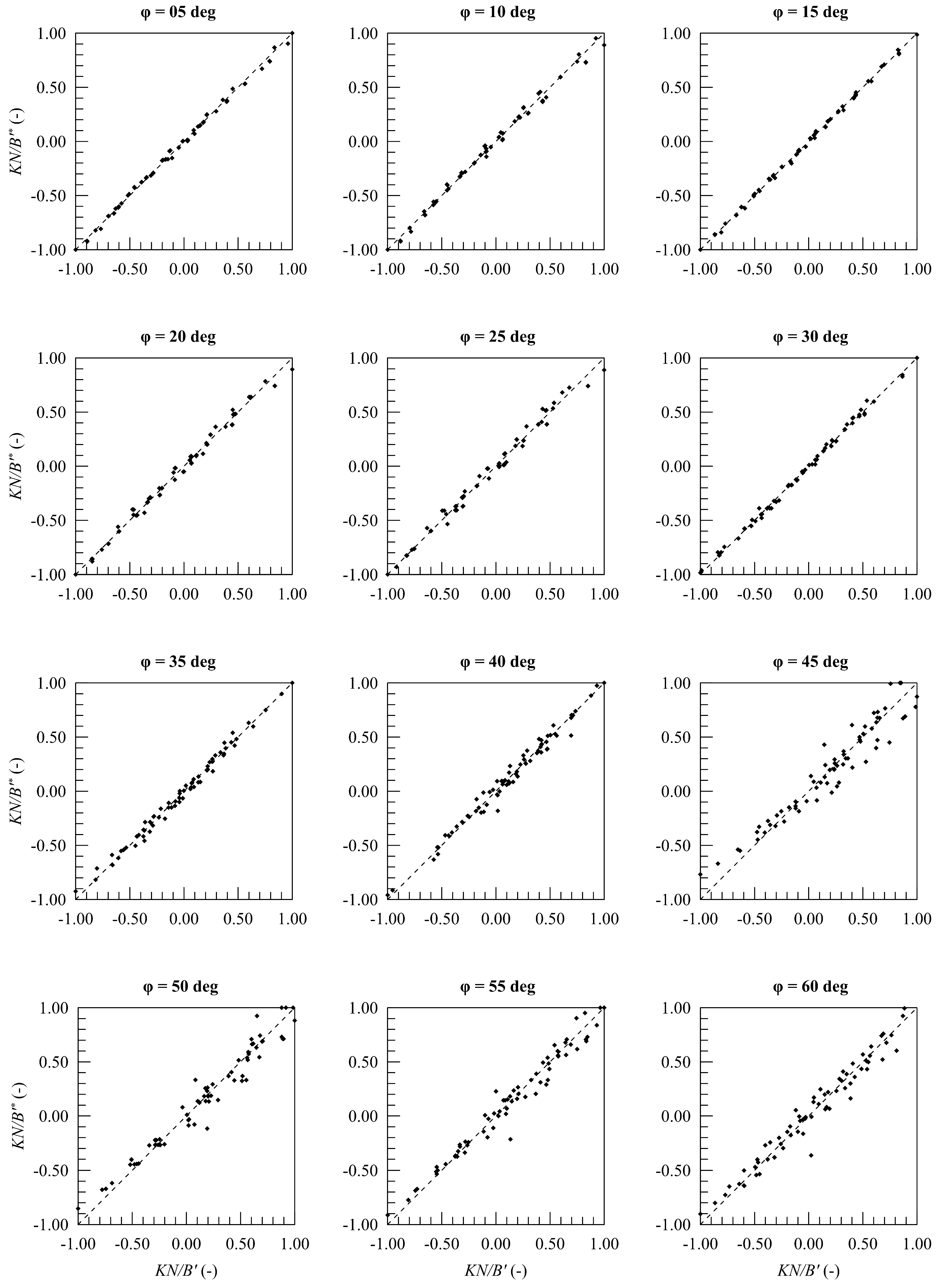
5.3. Metamodel Validation

The stability metamodel has been validated comparing the results obtained on two hull forms not included in the ship database but having geometrical parameters within the database ranges. The test hull forms, named Test 328 and Plume, are provided in Figure 8 together with their independent variables values and the non-dimensional cross curves of stability $KN/B$. The dashed lines relates to the cross curves of stability directly evaluated from the hull forms, while the black dots are the values predicted according to the proposed regression model. The stability metamodel shows a very good accuracy: the $R^2$ related to $KN/B$ is 0.9976 and 0.9979 for Test 328 and Plume, respectively. Also the results for $KM/B$ are very accurate. For Test 328, an observed $KM/B=0.628$ corresponds to a $0.630$ predicted one, whereas for Plume the observed value is $0.628$ and the predicted one is $0.609$. According to these results, the comparison between the predicted and the observed (i.e., directly computed) results can be considered satisfactory for the concept design stage.

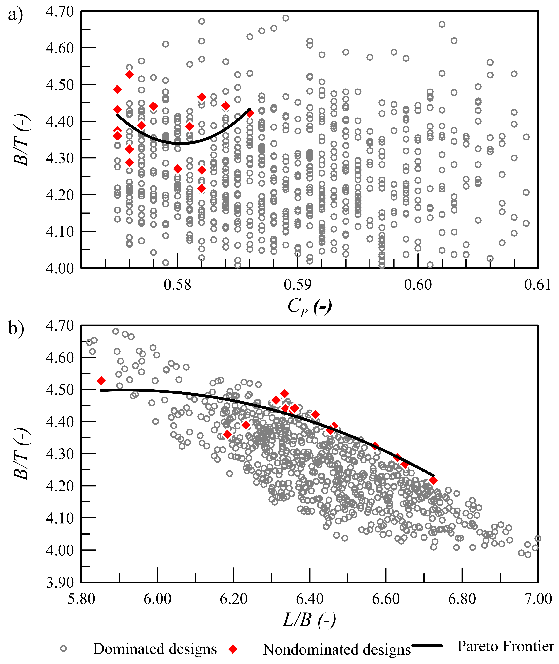
6. Results and Discussion

In this section, the results obtained applying the MADM methodology for the concept design of an LCTC involved in the selected North Europe—Mediterranean transport scenario are provided and discussed. 10,000 design alternatives have been generated by applying random Monte Carlo sampling to the design variables. Among them, 758 feasible design passed the constraint selection. It is worth noting that 1,260 designs have been eliminated due to intact stability lack (non compliant with IS Code [32]), showing the relevance of this aspect in the LCTC concept design. In order to check the compliance with Weather Criterion the following assumptions have been done: the actual lateral wind area has been calculated according to the midship section height; besides, all the alternative designs are equipped with bilge keels having an area equal to 2.5% of the waterplane area. Then, the feasible alternatives have been tested by dominance, so defining the Pareto frontier, which consists of 16 non-dominated designs.

Table 7. Main characteristics of non-dominated ships.

${\mathit{N}}_{\mathit{d}\mathit{e}\mathit{s}}$	${\mathit{L}}_{\mathit{B}\mathit{P}}$ (m)	B (m)	T (m)	$\mathbf{\Delta }$ (t)	$\mathit{L}/\mathit{B}$ $(-)$	$\mathit{B}/\mathit{T}$ $(-)$	${\mathit{C}}_{\mathit{B}}$ $(-)$	${\mathit{C}}_{\mathit{P}}$ $(-)$	${\mathit{C}}_{\mathit{V}\mathit{P}}$ $(-)$	${\mathit{C}}_{\mathit{W}\mathit{P}}$ $(-)$	${\mathit{N}}_{\mathit{c}\mathit{a}\mathit{r}}$ $(-)$	${\mathit{N}}_{\mathit{d}\mathit{e}\mathit{s}}$
15	220.478	34.934	7.822	34,790	6.311	4.466	0.561	0.582	0.707	0.793	8762	15
22	225.647	33.932	7.946	35,033	6.650	4.270	0.560	0.580	0.690	0.811	9176	22
183	225.543	34.018	7.933	34,798	6.630	4.288	0.556	0.576	0.703	0.790	9176	183
184	222.772	35.169	7.839	35,049	6.334	4.487	0.555	0.575	0.691	0.803	8969	184
213	227.721	34.242	8.025	36,096	6.650	4.267	0.561	0.582	0.706	0.794	9176	213
226	219.866	34.698	7.813	34,201	6.336	4.441	0.558	0.578	0.700	0.796	8762	226
343	221.618	34.866	7.866	34,683	6.356	4.432	0.555	0.575	0.710	0.781	8969	343
347	224.711	34.198	7.909	34,721	6.571	4.324	0.555	0.576	0.687	0.808	8969	347
410	225.051	35.385	7.967	36,766	6.360	4.442	0.563	0.584	0.705	0.798	9176	410
414	220.530	34.380	7.775	34,289	6.415	4.422	0.565	0.586	0.703	0.804	8762	414
420	223.209	34.537	7.875	34,962	6.463	4.386	0.560	0.581	0.707	0.792	8969	420
430	228.178	35.354	8.082	37,193	6.454	4.374	0.554	0.575	0.700	0.792	9176	430
543	216.833	34.791	7.928	34,204	6.232	4.389	0.556	0.577	0.709	0.784	8762	543
600	216.021	36.913	7.808	35,574	5.852	4.527	0.555	0.576	0.689	0.806	9117	600
706	216.350	34.990	8.026	34,661	6.183	4.360	0.554	0.575	0.708	0.783	8762	706
724	227.310	33.808	8.016	35,550	6.724	4.217	0.561	0.582	0.685	0.818	9176	724
${\mathit{N}}_{\mathit{d}\mathit{e}\mathit{s}}$	$\mathit{M}\mathit{D}\mathit{O}$ (t/h)	$\mathit{E}\mathit{E}\mathit{D}\mathit{I}$ (a/r)	$\mathit{P}\mathit{o}\mathit{w}\mathit{c}\mathit{f}$ $(-)$	$\mathit{W}\mathit{B}$ (t)	$\mathit{W}\mathit{e}\mathit{a}\mathit{t}\mathit{h}.$ $\mathit{C}\mathit{r}\mathit{i}\mathit{t}.$	${\ddot{\mathbf{\zeta }}}_{\mathit{w}\mathit{h}}$ (m/s2)	${\mathit{I}}_{\mathit{t}}$ $(-)$	${\mathbf{\mu }}_{\mathit{v}\mathit{i}\mathit{b}}$ $(-)$	$\mathit{C}\mathit{a}\mathit{p}\mathit{e}\mathit{x}$	$\mathit{O}\mathit{p}\mathit{e}\mathit{x}$	$\mathit{R}\mathit{F}\mathit{R}$ (USD/car 1000 nm)	${\mathit{N}}_{\mathit{d}\mathit{e}\mathit{s}}$
									(mmUSD)
15	2.413	0.559	1.414	4426	1.454	0.47	0.149	0.863	66.83	13.64	64.691	15
22	2.414	0.560	1.411	4193	1.549	0.50	0.159	0.538	66.90	13.72	63.857	22
183	2.415	0.562	1.400	3942	1.377	0.48	0.159	0.612	66.94	13.73	63.988	183
184	2.413	0.556	1.415	4233	1.516	0.47	0.152	0.538	67.29	13.69	65.021	184
213	2.413	0.551	1.392	5039	1.636	0.49	0.161	0.502	67.38	13.73	63.409	213
226	2.414	0.566	1.416	3955	1.444	0.47	0.150	0.915	66.61	13.64	66.076	226
343	2.414	0.562	1.402	4050	1.453	0.46	0.152	0.902	66.96	13.69	64.847	343
347	2.414	0.562	1.413	4096	1.441	0.49	0.158	0.567	66.94	13.68	64.834	347
410	2.497	0.581	1.402	5454	1.616	0.48	0.153	0.555	68.29	14.05	64.319	410
414	2.413	0.562	1.425	4070	1.440	0.48	0.150	0.669	66.47	13.64	66.384	414
420	2.413	0.558	1.408	4314	1.451	0.48	0.154	0.674	66.95	13.68	64.832	420
430	2.497	0.580	1.387	5728	1.618	0.47	0.159	0.626	68.72	14.05	64.751	430
543	2.416	0.571	1.402	4173	1.449	0.45	0.149	0.997	66.33	13.64	66.523	543
600	2.497	0.590	1.426	4465	1.498	0.44	0.140	0.987	68.02	14.03	64.458	600
706	2.414	0.570	1.396	4634	1.432	0.44	0.149	0.999	66.42	13.64	66.067	706
724	2.413	0.557	1.410	4656	1.553	0.51	0.162	0.508	67.04	13.72	63.529	724

reports the main characteristics of the non-dominated ships, which represent the most promising solutions for the selected transport scenario. The results provide some interesting insights regarding the ship main particulars, and can be applied to better define the design space in the LCTC concept design.

Figure 9a shows the distribution of the $RFR$ as a function of the ship displacement $\Delta$. The non-dominated results belong to a lower envelope curve enclosing the feasible region, allowing quite clear identification of the Pareto frontier. Such a curve shows a minimum value, corresponding to the lower $RFR$ obtained in the selected transport scenario. Hence, the corresponding displacement identifies the best size of the LCTC vessel corresponding to design parameters. It is worth noting, that for both larger and smaller vessels the economic performances of the vessel decrease, highlighting the importance of MADM to define the best possible solution in a given operating scenario.

Moreover, some additional considerations can be done regarding hull geometry and the main particulars adopted for its definition in the concept design. Figure 9b and Figure 10c provides the $RFR$ and $B/T$ ratio as a function of $C_P$, respectively. In these cases, a clear definition of the Pareto frontier is not possible. Nevertheless, all the non-dominated designs are gathered in a specific region of the design space identified by $B/T\in [4.20,4.55]$ and $C_P\in [0.57,0.59]$. Hence, for the selected transport scenario, a deeper analysis might be done in that design subspace to search for additional design alternatives laying on the Pareto frontier.

Finally, Figure 10d shows the relation between $L/B$ and $B/T$. Here, again, a quite good correlation can be identified among the non-dominated designs. In detail, it can be concluded that the best possible solution shall be searched within $L/B\in [6.20,6.80]$, whereas the $B/T$ can be preliminarily assessed as a function of $L/B$ as:

$$\frac{B}{T}=-0.599\frac{L}{B}+8.252$$

(16)

The results concerning economics attributes of the best-feasible ships deserve further insights. First, the MDO fuel consumption shall be considered; as it is noted in Table 7, the lowest value is 2.413 t/h, whilst the highest is equal to 2.497 t/h, thus the difference is 0.084 t/h. Considering an LCTC ship, 280 running days per year can be supposed [35], which means $280\times 24=6720\mathrm{h}/\mathrm{year}$. For a 20-year design lifetime, without taking into account neither the added fuel consumption due to the decrease of efficiency nor the bunkering price variations along the lifetime, the overall consumption in first approximation equals to $6720\times 20\times 0.084=11,290\mathrm{t}$. With an average MDO price of $\approx 400\mathrm{USD}/\mathrm{t}$, the saving of 4.5 million USD for each ship is not to be neglected. It is worth noting that all the designs laying on the Pareto frontier are characterised by a low fuel consumption, hence, the savings increase remarkably if these designs are compared with any other feasible alternative.

Further discussions can be made analysing a specific ship and comparing her attributes to the other non-dominated designs’ ones. For instance, the ship $N_{des}=600$ has the worst fuel consumption leading to an $OPEX$ close to the highest value. Moreover, due to its dimensions, also the $CAPEX$ is quite high, while the $RFR$ is in the middle range. At first glance, the selected ship does not seem to be highlighted close to the “preferred ships”, but the mathematical model has considered her for other attributes, that must be taken into account in the transport scenario. Indeed, ship $N_{des}=600$ corresponds to the best $EEDI$ index, the lowest vertical accelerations and one of the highest number of cars transported, being preferred for the environment, comfort and capacity attributes more than for propulsion dependent ones. Hence, the proper selection of the design attributes is of the utmost importance to properly balance the conflicting technical and economical requirements of a new LCTC.

It shall be noted that changing the transport scenario and the design parameters, different results can be obtained. Hence, the presented findings concerning the ship geometry cannot be universally applied because are strictly related to both the operating environment and the technical requirements described with the design parameters. However, the results show clearly the importance of a robust concept design methodology to define the main characteristics of an LCTC in order to assure the economic success of a new design in a defined operating scenario.

7. Conclusions

This work provides an application of MADM methodology within the concept design of an LCTC vessel. The paper shows how the main geometry particulars defining the hull forms have a strong influence not only on the ship technical performances, but also on the profit of the shipping company. A proper assessment during the concept design stage is compulsory since in the next design phases these parameters cannot be changed without significant waste of time and resources. Considering the vehicle transport between North Europe and the Mediterranean region, the optimal size of an LCTC has been assessed. The best possible solution has a displacement of about 36,000 t which corresponds to an $RFR$ of about 63.50 USD per car and 1000 nm. This finding is particularly interesting since shows that in a given operating scenario an optimal vessel size can be defined. Hence, the continuous increase of LCTC size shall be considered with the due care, limiting the current run towards gigantism. Nevertheless, in the studied transport scenario, the overall length of the most profitable solution exceeds the limit of 200 m in length, which is usually applied to PCTCs.

Besides, the paper explores a methodology to properly address the stability issues in the LCTC concept design. The proposed approach, based on MLR, provides an estimation of both the cross curves $KN$ and the transversal metacentre height $KM$ of the ship from its main particulars, without requiring the detailed definition of the hull forms (usually carried out during the next preliminary design stage). The method is independent by the ship loading condition, which is assessed by other dedicated metamodels that can be further described in future works. Hence, the applicability range of the proposed stability metamodel is enlarged compared to other models having the $KG$ as independent variable. The stability metamodel has been found satisfactory by comparing its results with the direct calculations of the $KN$ curves and the metacentre height $KM$ carried out for the two geometries not included in the ships’ database. The importance of stability issues in LCTC concept design is emphasised by the large number of design alternatives that have been rejected due to non-compliance with stability rules (more than 12% of the generated alternatives).

In conclusion, the paper shows once again the importance of the concept design phase to properly adapt the new vessel to a seaborne transport scenario. The MADM approach and the Pareto filtering enable to define subspaces where a more deep analysis can be carried out and to select the most promising feasible design solutions, which shall be considered by shipping companies decision-makers. Here, the best possible solution is the one that minimizes the $RFR$, which is adopted as the economic measure of merit. However, it shall be noted that in the present study some crucial aspects, such as ship motions, have not been extensively considered. The LCTC seakeeping metamodel only accounts for the maximum accelerations in the region having the most severe sea conditions encountered during the voyage (the Biscay Gulf). Since the seakeeping capabilities of the vessel are directly related to cargo losses, a more extensive study of the topic and a proper modelling within the MDM is advisable. Such aspects must be addressed in future works as well as a deeper exploration of the tight design subspace where non-dominated designs are located.

References

1. Pugh, S. Total Design: Integrated Methods for Successful Product Engineering; Addison-Wesley: Wokingham, UK, 1991. [Google Scholar]
2. Vicenzutti, A.; Trincas, G.; Bucci, V.; Sulligoi, G.; Lipardi, G. Early-Stage design methodology for a multirole electric propelled surface combatant ship. In Proceedings of the 2019 IEEE Electric Ship Technologies Symposium (ESTS), Washington, DC, USA, 14–16 August 2019; pp. 97–105. [Google Scholar] [CrossRef]
3. Trincas, G.; Mauro, F.; Braidotti, L.; Bucci, V. Handling the path from concept to preliminary ship design. In Proceedings of the Marine Design XIII, Helsinki, Finland, 10–14 June 2018; Volume 1, pp. 181–192. [Google Scholar]
4. Žanić, V.; Grubišić, I.; Trincas, G. Multiattribute decision-making system based on random generation of non-dominated solutions: An application to fishing vessel design. In Proceedings of the 3rd International Symposium on Practical Design of Ships and Mobile Units—PRADS’92, Newcastle upon Tyne, UK, 17–22 May 1992; pp. 623–630. [Google Scholar]
5. Trincas, G.; Grubišić, I.; Žanić, V. Comprehensive concept design of fast ro-ro ships by multiattribute decision making. In Proceedings of the 5th International Marine Design Conference—IMDC’94, Delft, The Netherlands, 24–27 May 1994; pp. 403–418. [Google Scholar]
6. Žanić, V.; Čudina, P. Multiattribute Decision Making Methodology in the Concept Design of Tankers and Bulk Carriers. Brodogradnja 2009, 60, 19–43. [Google Scholar]
7. Jafaryeganeh, H.; Ventura, M.; Guedes Soares, C. Application of multi-criteria decision making methods for selection of ship internal layout design from a Pareto optimal set. Ocean. Eng. 2020, 202, 107151. [Google Scholar] [CrossRef]
8. Trincas, G. Optimal fleet composition for marine transport of compressed natural gas from stranded fields. In Proceedings of the 2nd INT NAM Conference, Istanbul, Turkey, 23–24 October 2014; pp. 25–38. [Google Scholar]
9. Arias, C.; Herrador, J.; del Castillo, F. Intact and damage stability assessment for the preliminary design of a pasenger vessel. In Proceedings of the 8th International Conference on the Stability of Ships and Ocean Vehicles, STAB 2003, Madrid, Spain, 15–19 September 2003. [Google Scholar]
10. Mauro, F.; Braidotti, L.; Trincas, G. A Model for Intact and Damage Stability Evaluation of CNG Ships during the Concept Design Stage. J. Mar. Sci. Eng. 2019, 7, 450. [Google Scholar] [CrossRef] [Green Version]
11. Rodrigue, J.P. The Geography of Transport Systems; Routledge: New York, NY, USA, 2020. [Google Scholar]
12. Trincas, G. Survey of design methods and illustration of multiattributes decision making system for concept ship design. In Proceedings of the MARIND 2001, Varna, Bulgaria, 1–4 October 2001. [Google Scholar]
13. Mauro, F.; Braidotti, L.; Trincas, G. Effect of Different Propulsion Systems on CNG Ships Fleet Composition and Economic Effectiveness. In Proceedings of the 19th International Conference on Ship & Maritime Research, NAV 2018, Trieste, Italy, 20–22 June 2018. [Google Scholar] [CrossRef]
14. Jafaryeganeh, H.; Ventura, M.; Guedes Soares, C. Effect of normalization techniques in multi-criteria decision making methods for the design of ship internal layout from a Pareto optimal set. Struct. Multidiscip. Optim. 2020, 62, 1849–1863. [Google Scholar] [CrossRef]
15. Zadeh, L. Fuzzy Sets. Inf. Control. 1965, 8, 338–353. [Google Scholar] [CrossRef] [Green Version]
16. Bertram, V. Estimating Main Dimensions and Coefficients in Preliminary Ship Design. Schiffstechnik 1998, 45, 96–98. [Google Scholar]
17. Alkan, A.; Trincas, G.; Nabergoj, R. Seakeeping metamodel of fast ro-ro ships: RSM or ANN technique? In Proceedings of the 12th International Congress of the International Maritime Association of the Mediterranean, IMAM 2005, Lisboa, Portugal, 26–30 September 2005; pp. 789–797. [Google Scholar]
18. Mauro, F.; Braidotti, L.; Trincas, G. Determination of an optimal fleet for a CNG transportation scenario in the Mediterranean Sea. Brodogradnja 2019, 70, 1–23. [Google Scholar] [CrossRef]
19. Novak, V. Fuzzy Sets and Their Applications; Adam Hilger: Bristol, UK, 1989. [Google Scholar]
20. Buxton, I. Engineering Economics and Ship Design. In Engineering Economics and Ship Design; British Maritime Technology Ltd.: Feltham, UK, 1987; Chapter 2; pp. 79–95. [Google Scholar] [CrossRef]
21. Benford, H. The Practical Application of Economics to merchant Ship Design. Mar. Technol. 1967, 4, 519–536. [Google Scholar]
22. Buxton, I. Thirteen Graduate School; Chapter Cost Analysis as Applied to All Types of Marine Vehicles; West European Graduate Education in Marine Technology: Delft, The Netherlands, 1989. [Google Scholar]
23. Carreyette, J. Preliminary Ship Cost Estimation. Trans. RINA 1977, 119, 235–258. [Google Scholar]
24. Grubišić, I.; Žanić, V.; Trincas, G. Sensitivity of multiattribute design to economy enviroment: Shortsea Ro-Ro vessels. In Proceedings of the 6th International Marine Design Conference—IMDC’97, Espoo, Finland, 10–14 June 1997; pp. 201–216. [Google Scholar]
25. Papanikolaou, A. Holistic ship design optimization. Comput. Aided Des. 2010, 42, 1028–1044. [Google Scholar] [CrossRef]
26. Goss, R. Economic Criteria for Optimal Ships Designs. Trans. RINA 1965, 107, 581–596. [Google Scholar]
27. Aspen, D.; Sparrevik, M.; Magerholm Fet, A. Review of methods for sustainability appraisals in ship acquisition. Environ. Syst. Decis. 2015, 35, 323–333. [Google Scholar] [CrossRef] [Green Version]
28. Shetelig, H. Shipbuilding Cost Estimation: Parametric Approach; Technical Report; Norvegian Univeristy of Science and Technology: Trondheim, Norway, 2013. [Google Scholar]
29. Chatterjee, S.; Simonoff, J.S. Multiple Linear Regression. In Handbook of Regression Analysis; John Wiley & Sons, Ltd.: Hoboken, NJ, USA, 2013; Chapter 1; pp. 1–21. [Google Scholar] [CrossRef]
30. Lai, T.L.; Robbins, H.; Wei, C.Z. Strong consistency of least squares estimates in multiple regression. Proc. Natl. Acad. Sci. USA 1978, 75, 3034–3036. [Google Scholar] [CrossRef] [PubMed] [Green Version]
31. Harrell, F. Regression Modelling Strategies: With Application to Linear Models, Logistic Regression, and Survival Analysis; Springer: New York, NY, USA, 2001. [Google Scholar]
32. IMO. Intact Stability Code; International Maritime Organization: London, UK, 2008. [Google Scholar]
33. Chang, H. A data mining approach to dynamic multiple responses in Taguchi experimental design. Expert Syst. Appl. 2008, 35, 1095–1103. [Google Scholar] [CrossRef]
34. Box, G.E.P.; Wilson, K.B. On the Experimental Attainment of Optimum Conditions. J. R. Stat. Soc. Ser. B Methodol. 1951, 13, 1–45. [Google Scholar] [CrossRef]
35. Bialystocki, N.; Konovessis, D. On the estimation of ship’s fuel consumption and speed curve: A statistical approach. J. Ocean. Eng. Sci. 2016, 1, 157–166. [Google Scholar] [CrossRef] [Green Version]
36. Hogben, N.; Dacunha, N.M.C.; Olliver, G. Global Wave Statistics; British Maritime Technology Ltd.: Feltham, UK, 1986. [Google Scholar]
37. Nomoto, K.; Taguchi, T.; Honda, K.; Hirano, S. On the Steering Qualities of Ships. Int. Shipbuild. Prog. 1957, 4, 354–370. [Google Scholar] [CrossRef]
Figure 1. LCTC Considered Route.
Jmse 09 00278 g001
Figure 2. Feasibility flowchart for the Mathematical Design Model.
Jmse 09 00278 g002
Figure 3. Framework for Metamodels.
Jmse 09 00278 g003
Figure 4. Cumulative Density Function of the C W P , the C V P and T / D parameter.
Jmse 09 00278 g004
Figure 5. Body plans of one sub-family of ships having similar hull forms.
Jmse 09 00278 g005
Figure 6. Predicted /observed values for the K N / B regressions.
Jmse 09 00278 g006
Figure 7. Absolute value of regression coefficients normalised in [ 0 , 1 ] .
Jmse 09 00278 g007
Figure 8. Test body plans, main particulars and comparison of the predicted and observed non-dimensional cross curve of stabilty.
Jmse 09 00278 g008
Figure 9. Distribution of the RFR of the feasible LCTC design alternatives as a function of displacement (a) and prismatic coefficient (b).
Jmse 09 00278 g009
Figure 10. Distribution of breadth-draught ratio as a function of prismatic coefficient (a) and lenght-breadth ratio (b).
Jmse 09 00278 g010