Article

Revisit of a Case Study of Spilled Oil Slicks Caused by the Sanchi Accident (2018) in the East China Sea

1
Marine Science and Technology College, Zhejiang Ocean University, Zhoushan 316022, China
2
College of Marine Sciences, Shanghai Ocean University, Shanghai 201306, China
3
National Satellite Ocean Application Service, Beijing 100081, China
4
National Marine Data and Information Service, Tianjin 300171, China
5
South China Sea Institute of Oceanology, Chinese Academy of Sciences, Guangzhou 510301, China
*
Authors to whom correspondence should be addressed.
J. Mar. Sci. Eng. 2021, 9(3), 279; https://0-doi-org.brum.beds.ac.uk/10.3390/jmse9030279
Submission received: 31 January 2021 / Revised: 25 February 2021 / Accepted: 26 February 2021 / Published: 4 March 2021
(This article belongs to the Special Issue Marine Oil Spills 2020)

Abstract

:
Marine oil spills occur suddenly and pose a serious threat to ecosystems in coastal waters. Oil spills continuously affect the ocean environment for years. In this study, the oil spill caused by the accident of the Sanchi ship (2018) in the East China Sea was hindcast simulated using the oil particle-tracing method. Sea-surface winds from the European Centre for Medium-Range Weather Forecasts (ECMWF), currents simulated from the Finite-Volume Community Ocean Model (FVCOM), and waves simulated from the Simulating WAves Nearshore (SWAN) were employed as background marine dynamics fields. In particular, the oil spill simulation was compared with the detection from Chinese Gaofen-3 (GF-3) synthetic aperture radar (SAR) images. The validation of the SWAN-simulated significant wave height (SWH) against measurements from the Jason-2 altimeter showed a 0.58 m root mean square error (RMSE) with a 0.93 correlation (COR). Further, the sea-surface current was compared with that from the National Centers for Environmental Prediction (NCEP) Climate Forecast System Version 2 (CFSv2), yielding a 0.08 m/s RMSE and a 0.71 COR. Under these circumstances, we think the model-simulated sea-surface currents and waves are reliable for this work. A hindcast simulation of the tracks of oil slicks spilled from the Sanchi shipwreck was conducted during the period of 14–17 January 2018. It was found that the general track of the simulated oil slicks was consistent with the observations from the collected GF-3 SAR images. However, the details from the GF-3 SAR images were more obvious. The spatial coverage of oil slicks between the SAR-detected and simulated results was about 1 km2. In summary, we conclude that combining numerical simulation and SAR remote sensing is a promising technique for real-time oil spill monitoring and the prediction of oil spreading.

1. Introduction

Marine oil spills are serious marine disasters that occur in marine ports, docks, and oil drilling platforms. Oil spills cause damage to the marine ecological environment and are a direct threat to public safety. Moreover, oil slicks drift with the movements of ocean circulations and ocean waves, causing oil pollution to persist in the ocean for a long time. In recent years, due to rapid economic development in China, the Chinese demand for crude oil and refined products is increasing year by year, leading to a high potential risk of marine oil spills. On 16 July 2010, an oil spill occurred in Dalian Xingang Port, leading to more than 1500 tons of oil spilling into the sea. The oil spill seriously affected the local fisheries, aquaculture, tourism, and shipping industry and caused huge economic losses to Dalian City. Oil slicks spilled from ships account for the major proportion of oil spill accidents. For example, the pollution in surrounding areas for up to 180 days and more than 50% of bulk oil particles remaining in the ocean after the Sanchi ship accident (2018) in the East China Sea were due to oil slicks [1]. Owing to the frequent occurrence of major oil spill accidents, the development of oil spill monitoring techniques has progressed in the last few decades. It is necessary to promote emergency responses to marine oil spills in China and improve oil slick simulation techniques.
Most studies involving spilled oil slick simulations have focused on the development of numerical models [2,3,4,5]. Several oil slick prediction models have been developed during the past 20 years and the state of the art in oil slick modeling has been reviewed by various studies [6,7,8], e.g., Monte Carlo stochastic simulation, Lagrangian transport, and the oil particle-tracing method. Generally, oil transportation is affected by marine environmental dynamic factors as well as the physical and chemical properties of oil, such as weathering [9], evaporation, and emulsification [10]. Compared with the previous algorithms for solving the convection diffusion equation, the oil particle-tracing method can not only solve the deformation and breaking process of oil spill under the influence of marine dynamic environment, but also accurately forecast the expansion process of oil film and the obvious stretch of oil film shape in the wind direction. Therefore, the most widely used oil spill model is based on the particle-tracing method, which simulates the drift and diffusion process of oil slicks in water by dispersing oil into a large number of small oil droplets [11,12]. In principle, the motion of oil particles is expressed by the Lagrange tracing method, and the implementation of this method could directly resolve the physical movement of oil slicks. The advantage of the oil particle-tracing method is that the shape changes and breaking process of oil slicks under the action of complex ocean environments is described while effectively eliminating the numerical divergence problem. However, prior knowledge of the oil particle-tracing method relies on sea-surface dynamics. It is well known that marine dynamic factors, such as sea-surface winds [13], currents [14], and waves [15,16,17], can be numerically simulated by high-resolution meteorological or hydrodynamic models.
With the development of remote-sensing technology, oceanic characteristics such as sea-surface temperature [18], chlorophyll-a [19], and sediment [20] content can be impressively imaged through optical satellites, including advanced very high-resolution radiometer (AVHRR) [21] and moderate-resolution imaging spectro-radiometer (MODIS) [22]. Satellites carrying microwave sensors, such as altimeters [23], scatterometers [24], and synthetic aperture radar (SAR) [25,26], can quantitatively detect information on ocean dynamics under all types of weather and in real time. In particular, it has been proven that SAR is greatly useful in oil spill monitoring [27,28,29,30,31], especially polarmetric SAR (PolSAR) [32], as well as the X-band marine radar [33] and the GNSS-R technique [34]. As for co-polarized SAR, the constant false alarm rate (CFAR) is a well-known method for oil spill detection [35]; the details are described in the Appendix A. Utilizing amplitude coherence and the co-polarized phase difference (CPD) standard deviation to detect the spilled oil slicks in dual-polarimetric TerraSAR-X imagery is proposed in [36]. After analyzing the backscattering differences between oil slicks and sea clutter, the feature pedestal height is used to observe oil slicks in quad-polarimetric SAR imagery [37]. Different from these two works, in [38], an advanced method for realizing oil spill detection from the compact polarimetric SAR image was recently developed. It is noteworthy that the accuracy of SAR detection for oil slicks relies on prior information about background dynamics to remove false alarms.
The efficiency of oil spill modeling based on the particle-tracing method for the case of the Dalian accident in July 2010 has been confirmed [39]. In recent studies of the Sanchi Event (2018), two individual methods, optical/microwave satellite and numerical modeling, have been widely employed [1,40]. In recent decades, these methods have been improved significantly. Therefore, the present work focused on the real-time monitoring and prediction of oil spills using SAR and numerical models, which are sound and can be practically applied for oil spills. It has also been revealed that the prediction accuracy of oil spill transportation depends on simulations from meteorological or hydrodynamic models. As for driving the oil spill model, the sea-surface wind, current, and wave fields are necessary. The oil particle drift mainly depends on sea-surface winds, tides, and circulation currents [41]. However, Stokes drift transport-induced ocean waves are also an important factor [42]. In this work, the coastal currents and waves associated with sea-surface wind were fully considered. The European Centre for Medium-Range Weather Forecasts (ECMWF) winds were directly employed, which have a good performance compared to moored measurements and satellite observations [43]. The ocean currents and waves were simulated using the Finite-Volume Community Ocean Model (FVCOM) [44] and the Simulating WAves Nearshore (SWAN) [45] model, respectively, which have a unique unstructured grid.
The rest of this paper is organized as follows. The data-set collection is described in Section 2, e.g., the forcing fields and open boundary data for modeling. In particular, the four Chinese Gaofen-3 (GF-3) SAR images acquired during the period of the Sanchi accident event were collected for this study. The method for spilled oil slick simulation using the particle-tracing model is introduced in Section 3. Also, the settings for the SWAN and FVCOM model are briefly described, and the validations of sea-surface currents and waves are presented. Moreover, the oil spill simulations are compared with the GF-3 SAR-detected results. The conclusions are summarized in Section 4.

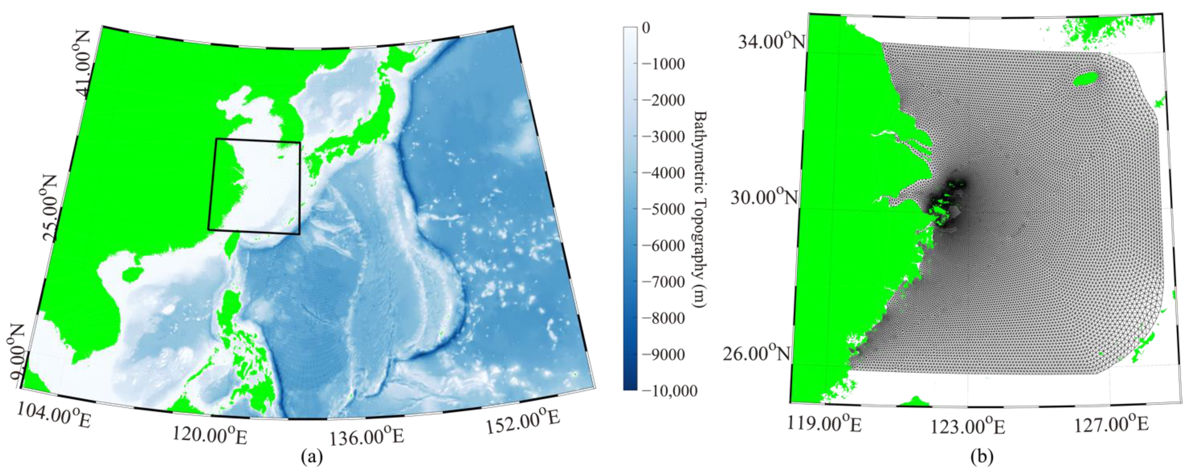
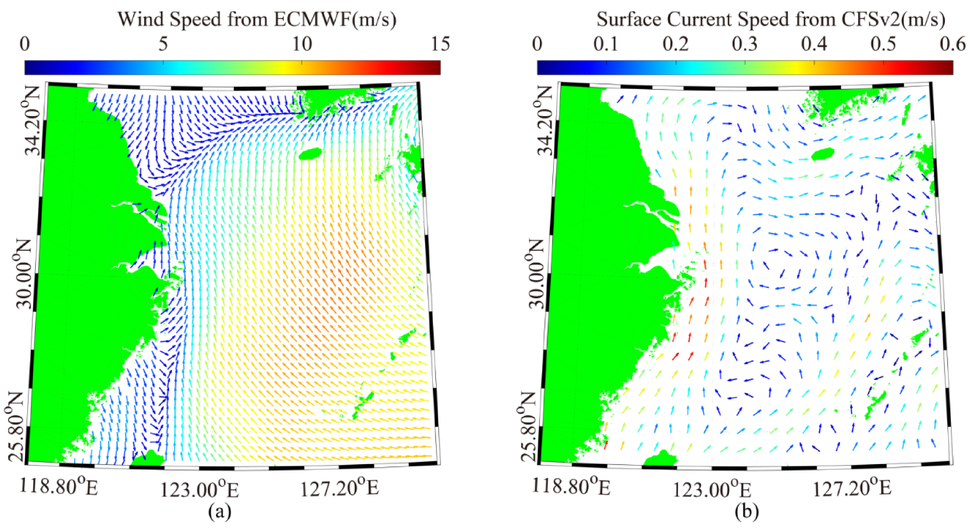
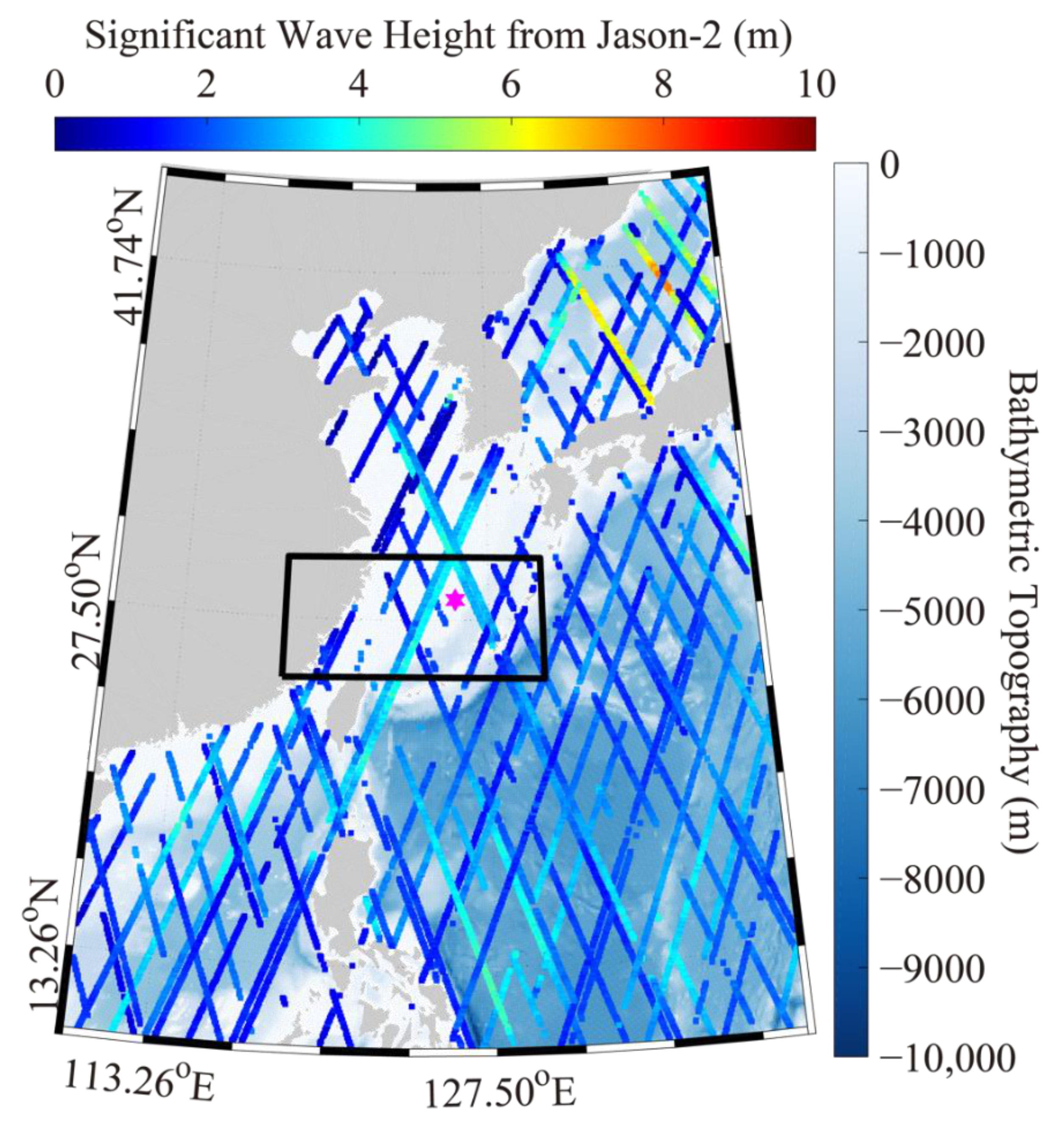
2. Dataset Collection

At 15:51 UTC on 6 January 2018, the oil tanker called Sanchi, carrying more than 100,000 tons of oil and natural gas, suddenly collided with a cargo ship called CF Crystal in the Zhoushan islands of the East China Sea [46], which is at the mouth of the Yangtze Estuary and Hangzhou Bay in China. Together with the collision, a large amount of spilled oil floated on the sea surface and spread as slicks. The geographic map of the spatial coverage of the Sanchi event is shown in Figure 1, in which the unstructured grids are uniquely used for sea-surface current and wave simulations using FVCOM and SWAN, respectively. The tidal current is relatively strong between Hangzhou Bay and the island chains due to the trumpet terrain. Moreover, it has been found that there are a series of smaller islands, resulting in the rapid change of wave properties. These background dynamic features of the regional marine environment cause difficulties in the prediction of oil-slicks.
In this study, the quick-look maps of four GF-3 SAR images during the period of 14–18 January 2018 after the shipwreck were collected, in which the pinkish marks represent the shipwreck positions, as shown in Figure 2. These images were acquired in Fine Stripmap (FS) mode with a spatial resolution of 10 m and a swath coverage of 100 km or Stander Stripmap (SS) mode with a spatial resolution of 25 m and a swath coverage of 130 km [47,48]. Generally, oil slicks contaminate the sea surface, where non-Bragg scattering dominates at such area whereas Bragg scattering dominates. In other words, the relatively low backscattering signal in a SAR image, expressed by normalized radar cross section (NRCS), is probably caused by oil slicks [49]. Collectively, the algorithms for the oil spill detection from a SAR image have been well established. The CFAR method is a mature method for co-polarized SAR application. In the collected SAR images, the irregular oil slicks are clearly visible, illustrated by low NRCS in Figure 2b to Figure 2c, which is useful for confirming the robustness of the spilled oil slick simulation using the oil particle-tracing method. However, other marine dynamics phenomena including eddies, fronts, and up-welling/down-welling can be also featured by low NRCS. As shown in Figure 2a, the cyclonic patterns of low NRCS are probably caused by the background marine dynamics, because the corresponding image was taken on the first day of shipwreck and the quantity of oil slicks are too small to produce the relatively large coverage of ‘low-NRCS’ compared to that on 15 January. In particular, the black oil-like patches with ‘low-NRCS’ in the GF-3 SAR image on 18 January (Figure 2d) were far away from shipwreck. Therefore, the images on 15 and 17 January were taken to confirm the oil slick simulation.
Since 1979, the ECMWF has continuously provided reanalysis wind data at 10 m above the sea surface with a 0.125° grid of spatial resolution at interval of 6 h each day, which is reliable for atmospheric and marine research. In particular, the ECMWF winds are popularly treated as the forcing field for running hydrodynamic models, such as FVCOM [44] for current simulation and SWAN [50] for wave simulation in this study. The case map of ECMWF wind taken at 00:00 on 16 January 2018 is shown in Figure 3a. The Climate Forecast System Version 2 (CFSv2) from the National Center of Atmospheric Research (NCAR) provided the sea-surface current data with about 50 km of spatial resolution, which was used for confirming the accuracy of the model-simulated currents from the FVCOM. Figure 3b shows the sea-surface current map from CFSv2 taken at 22:00 on 15 January 2018, in which the relatively strong current is clearly visible around the Zhoushan islands in the Yangtze Estuary. Similarly, the wave measurements from the Jason-2 altimeter were collocated with the model-simulated waves from SWAN in January 2018 in order to validate the model-simulated waves, although Jason-measured waves were available at the footprints following the satellite track, as shown in Figure 4, in which the pinkish marks represent the shipwreck position, and the black rectangle represents the available measurements for validating the model-simulated SWH from SWAN.

3. Method and Results

In this section, we present the simulated sea-surface current from the FVCOM model and the sea-surface wave from the SWAN model. The oil spill simulated using the oil particle-tracing method is then compared with SAR-detected oil slicks from GF-3 SAR images.

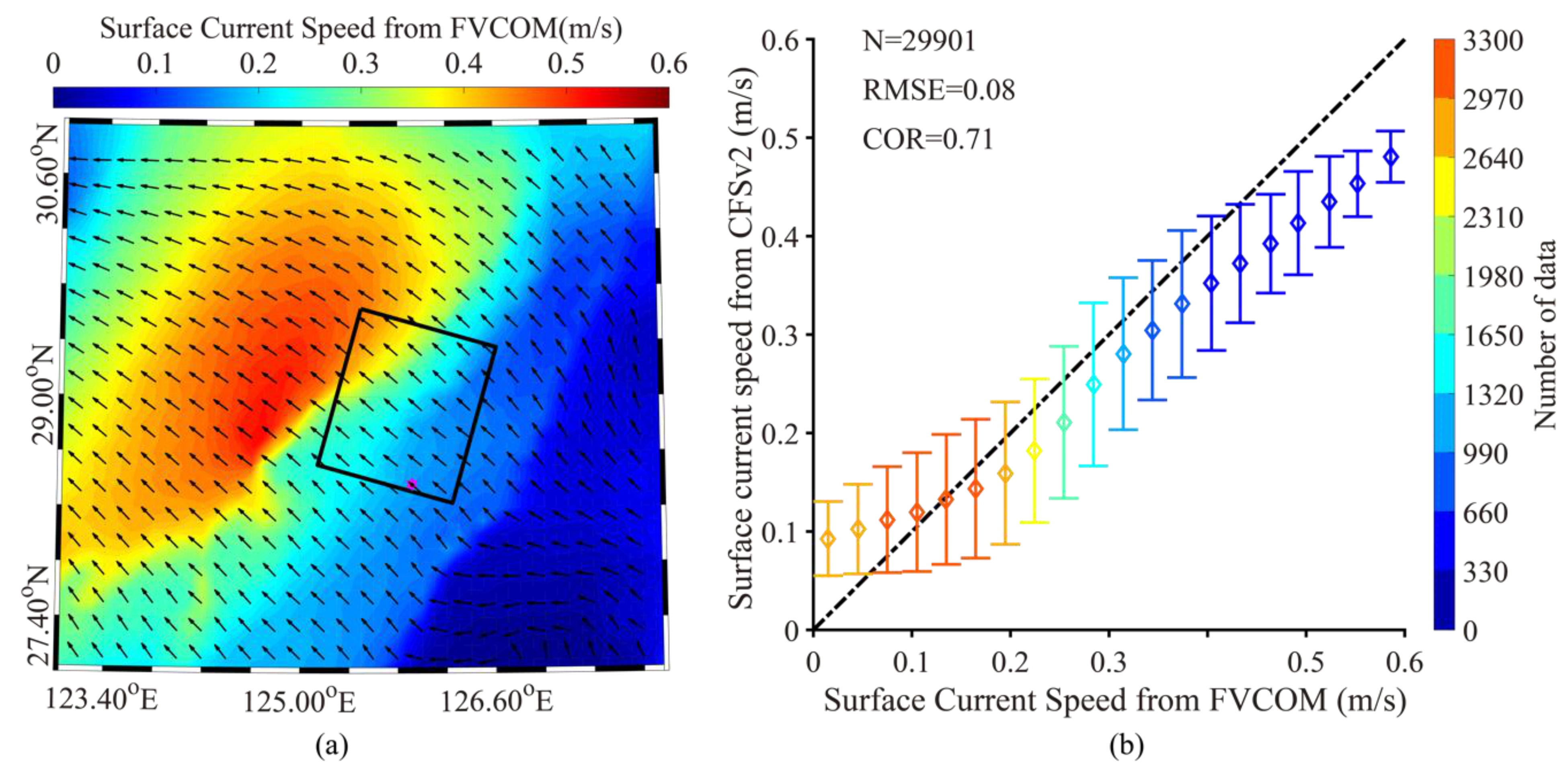
3.1. Simulation of Sea-Surface Current

In this work, the FVCOM model is used to simulate the sea-surface current, which follows the principle [44]:
dV dt + f V   =   1 p y + z K m V z + F ,  
dT dt   =   z K h T z + F T ,
dS dt   =   z K h S z + F S ,
ρ   =     ρ   T , S ,
u x + v y + w z   =   0   ,
where V is the velocity vector; u, v, and w are the components at x, y, and z coordinates; ρ is the sea-surface pressure; f is the Coriolis parameter; T is the sea temperature; S is the salinity; ρ is the sea water density; Km and Kh are the vertical eddy viscosity coefficient and he thermal vertical eddy diffusion coefficient, respectively; FT is the thermal term; and FS is the salt diffusion term. The winds from ECMWF with a 0.125° grid at a time interval of 6 h were the forcing field and the water depth was derived from bathymetric topography from the General Bathymetric Chart of the Oceans (GEBCO) at a 0.1° grid. The open boundary conditions included water tide data from TOPX.5; and sea-surface temperature, sea surface salinity, and sea surface current values from the HYbrid Coordinate Ocean Model (HYCOM) with 1/12° grid at a time interval of 1 h, as described in [14].
To confirm the applicability of the simulations, FVCOM-modeled sea-surface currents were compared with those from NCEP CFSv2. As an example, Figure 5a shows the sea-surface current map from FVCOM taken on 14 January at 22:30, in which the black rectangle represents the spatial coverage of the corresponding GF-3 SAR image and the pinkish marks represent the shipwreck position. Although the sea-surface current speed was less than 1 m/s, the distribution of sea-surface current was complex. Figure 3b shows the comparison of available matchups between sea-surface current speeds simulated by the FVCOM and the CFSv2 data in the black rectangle in Figure 3. Generally, it was also found that the model-simulated sea-surface current speeds were less than those from CFSv2, which was supposedly caused by the underestimation of the ECMWF winds [13]. However, the statistical analysis yielded a 0.08 m/s root mean square (RMSE) with a 0.71 correlation (COR), indicating that the sea-current simulated from FVCOM was suitable for conducting the spilled oil slick hindcasting for the Sanchi event.

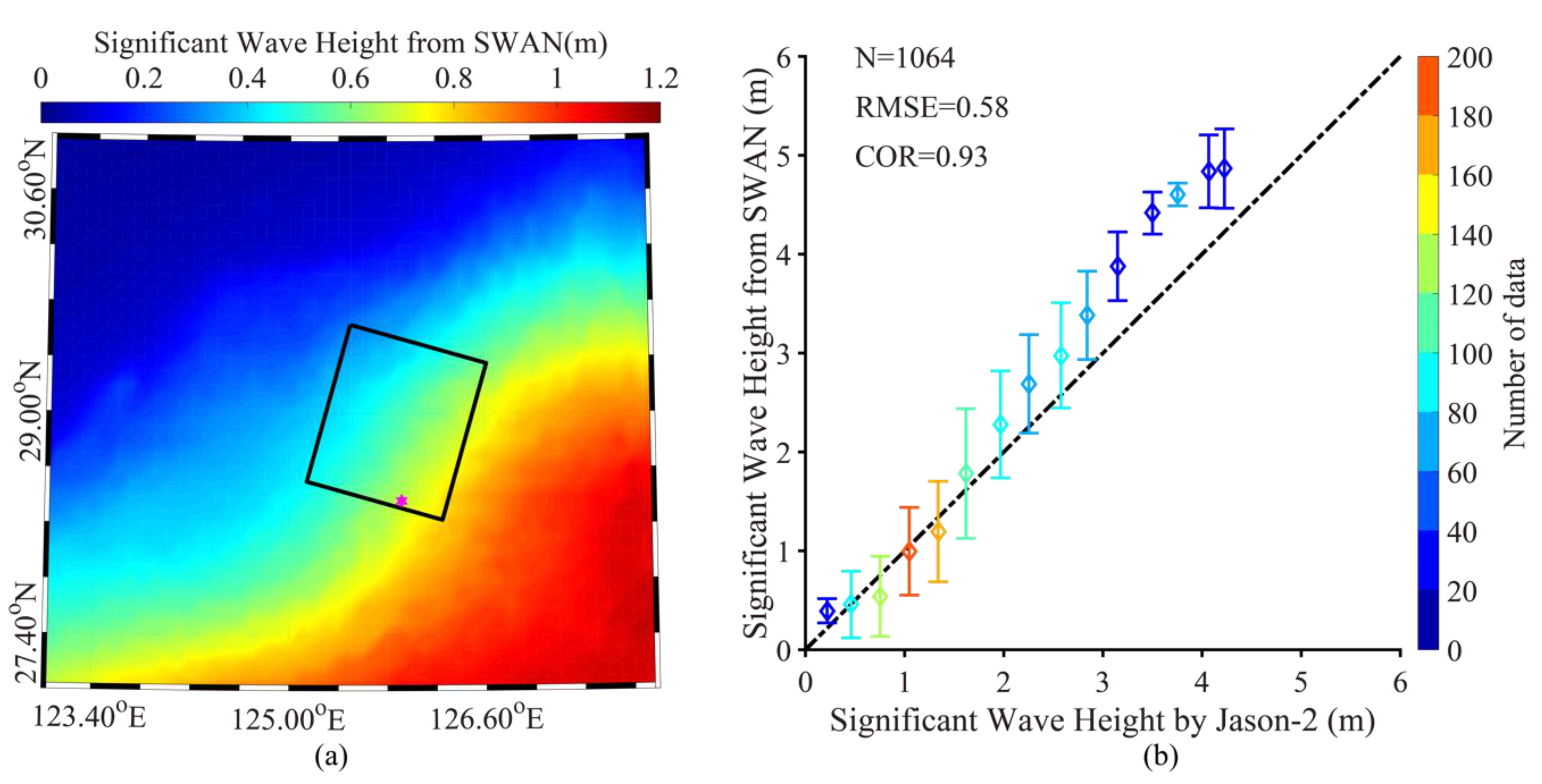
3.2. Simulation of Sea-Surface Wave

It is well known that the SWAN model has a good performance for sea-surface wave simulation in coastal waters. The governing equation of the SWAN model is expressed as:
D Dt N k , θ ; x , t   =   S i n + S b o t + S n l + S t q + S d b ,  
where N is the wave-density spectrum; k is the wave number; θ is the wave-propagation direction; x is the spatial vector; t is the temporary coordinate; Sin represents the wind-induced wave growth; Sbot represents the bottom-induced friction; Snl represents the nonlinear wave–wave interaction term; Stq represents the three- (triad) and four-wave components (quadruplets) of the wave–wave interactions; and Sdb represents dissipation induced by wave breaking. The parametric schemes follow [50]: wave interactions (QUADrupl); triad wave–wave interactions (TRIad); wave breaking (WESTHuysen); and bottom friction (JONWAP). ECMWF winds with a 0.125° grid at a time interval of 6 h were treated as a forcing field and the global bathymetric topography from GEBCO with a 0.1° grid was taken. The outputs were 0.1° grids with a 30-min temporal resolution. In particular, as proposed in [14], large changes in sea water level play an important role in wave simulation, as much as −0.5 m at the low sea state around Zhoushan islands. Therefore, the sea water level simulated from FVCOM was included in the wave simulation by the SWAN model.
According to the wave theory, SWH is a typical variable representing the energy of wave fields. The SWH map taken on 14 January at 22:30 is presented in Figure 6a, in which the black rectangle represents the spatial coverage of the corresponding GF-3 SAR image and the pinkish marks represent the shipwreck position. The model-simulated SWH from SWAN is compared with the collocated measurements from the Jason-2 altimeter, as shown in Figure 6b. It was found that the RMSE of SWH was 0.58 with a 0.93 COR. Again, the under-estimation of SWH, as SWH greater than 1.5 m, was probably caused by the inherent error of ECMWF winds.

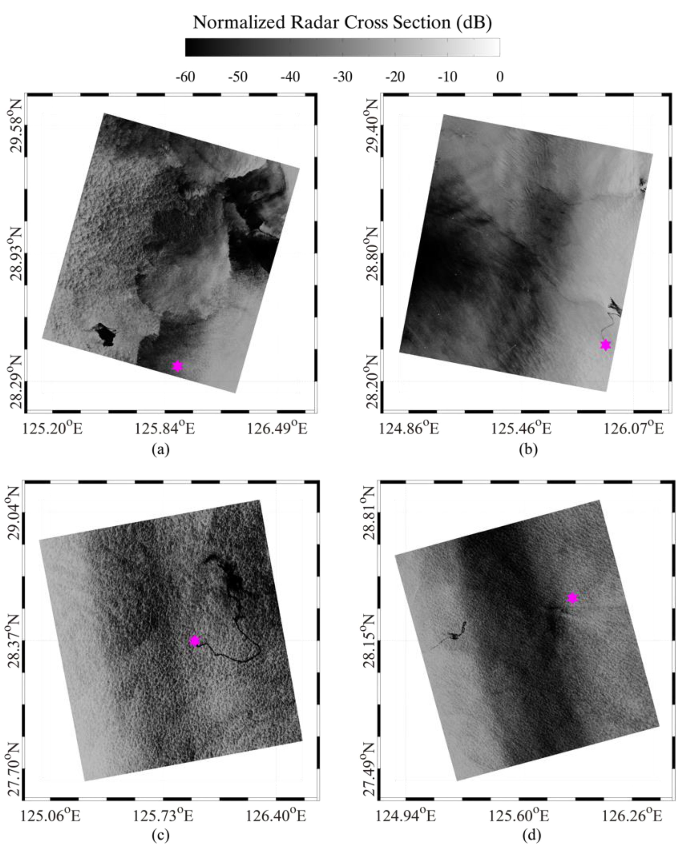
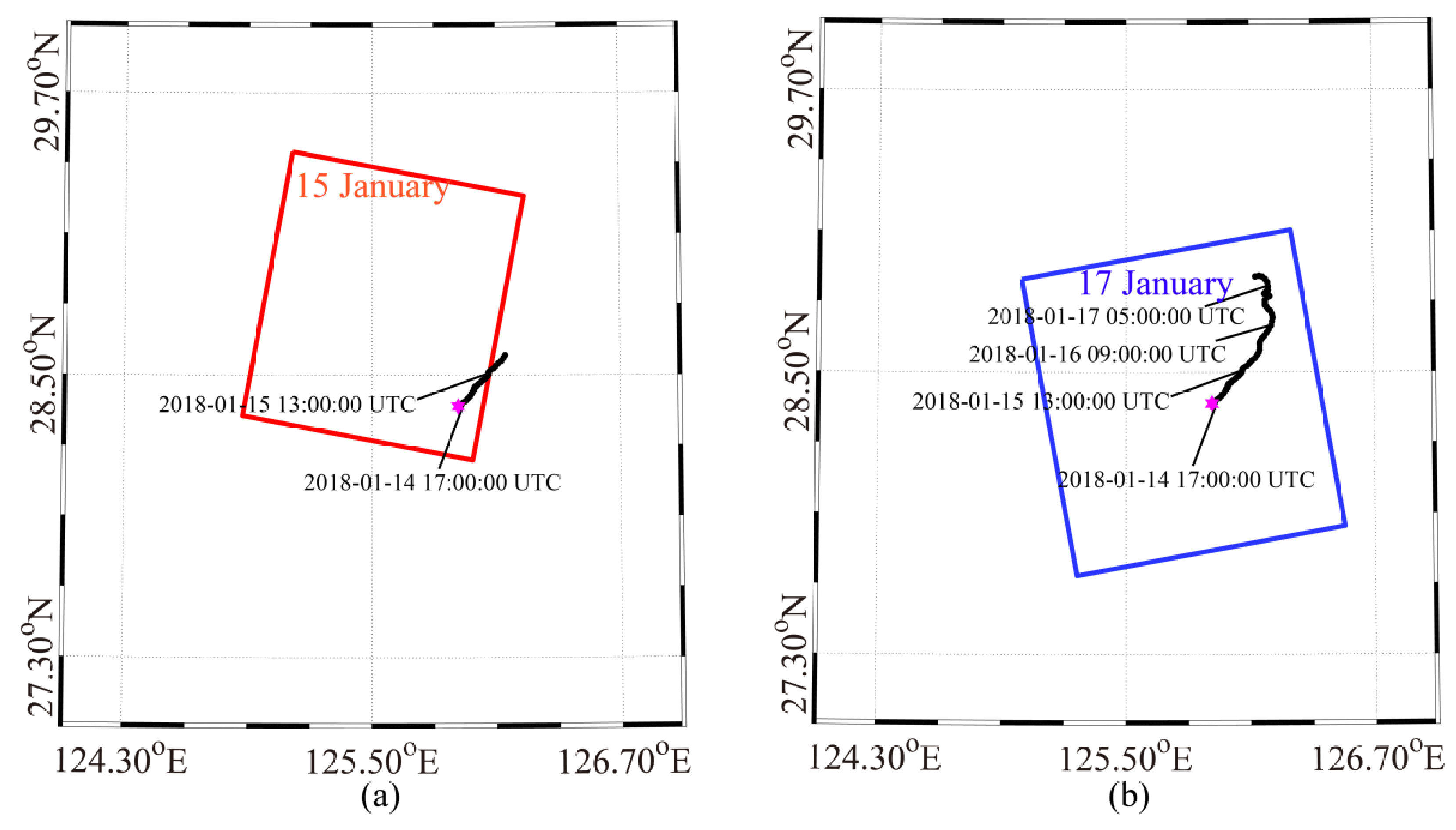
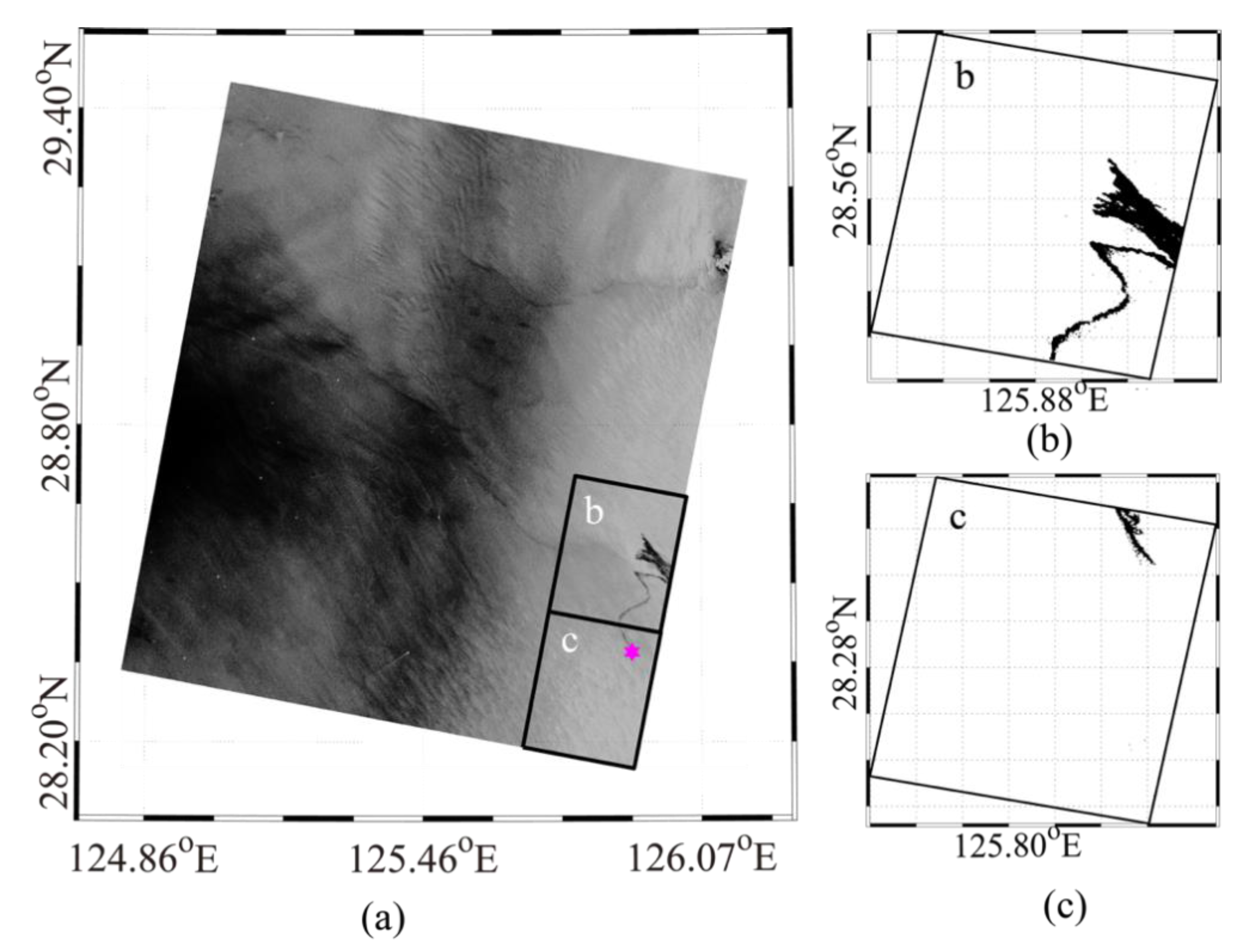
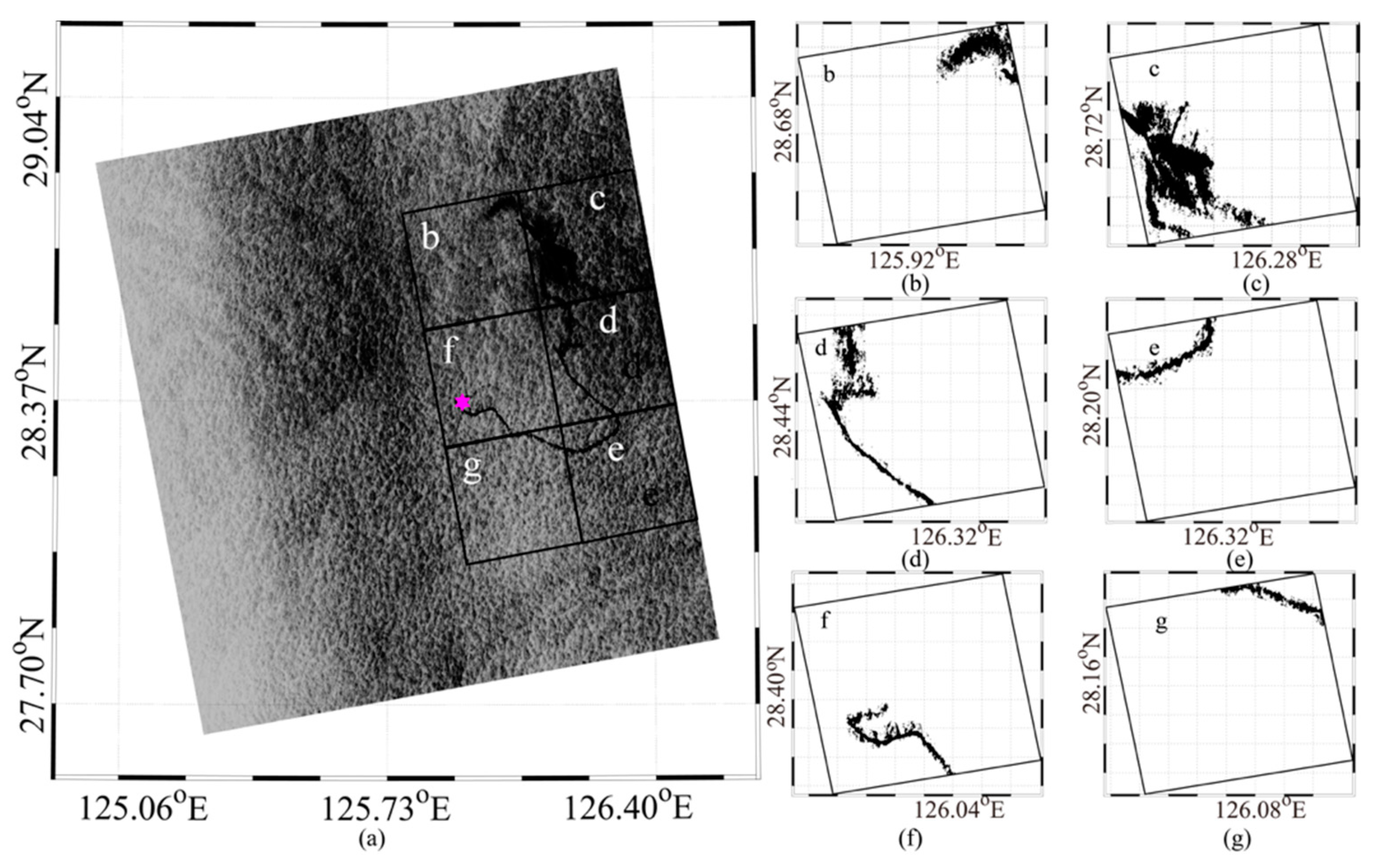
3.3. Simulation of Spilled Oil-Slicks

Traditionally, the empirical formula developed in [51] was adopted to simulate oil slicks spreading:
S   =   1 4 π MN ,  
where S is the oil slick area, and M and N are the lengths of the minor and major ellipse axis, respectively, given by:
M   =   1.13 ρ w ρ 0 ρ 0 1 / 3 V 0 1 / 3 t 1 / 4 ,  
N   =   M + 0.0034 U wind 4 / 3 t 1 / 4 ,  
where ρw is water density, ρ0 is oil density, V0 is the initial volume of spilled oil, t is the time after the oil slick commences spreading (min), and Uwind is wind speed. Let the concentric and similar ellipse, on which the particle is located, have major and minor axes n and m, respectively:
m M   =   n N .
If the coordinates of the particle relative to the principal axes of the ellipse are (X,Y), whose x-axis is selected in the direction of the wind, assuming X = ncosθ and Y = mcosθ, in which θ is the wind direction, then the oil particle is displaced outwards with the same elliptical angle, as follows:
Δ X   =   Δ ncos θ   =   Δ n X n   =   X Δ N N ,
Δ Y   =   Δ msin θ   =   Δ m Y m   =   Y Δ M M .
In this model, the drift and diffusion of spilled oil is solved by tracking a mass of oil particles equivalent to oil slicks. The position of each particle is affected by sea-surface winds, currents, and turbulent dispersion. The forecast model solves the following equation:
dx dt   =   V A X i , t + V D X i , t ,
where VA is advective velocity, VD is diffusive velocity, and Xi is particle position. VA is calculated as the linear combination of current velocity and wind speed as follows:
V A   =   V current + C D V wind ,
where Vcurrentis the sea-surface current velocity including tidal current, ocean current, and Stokes drift transport-induced waves [52,53], Vwind is the wind speed at 10-m height and CD is the wind drag coefficient. The turbulent diffusive velocity is calculated by Monte Carlo sampling in the range of velocities [-VD, VD], which are proportional to the diffusion coefficients. The velocity fluctuation at each time step Δ t is defined as:
V D   =   6 D Δ t ,
in which D is the diffusion coefficient and assumed to be 0.75 for this study.
In the Sanchi event, the shipwreck began on 14 January, and the total tons of condensate oil was about 13,6000 tons. Figure 7a shows the spreading track of simulated oil slicks using the oil particle-tracing method during the period 14–15 January 2018, and Figure 7b shows the period of 14–17 January 2018.Similarly, the SAR-detected oil slicks from the three collected GF-3 images are presented in Figure 8 and Figure 9. Although the oil slick simulation was generally consistent with SAR-detected results, the details of spilled oil slicks were clearly extracted from the GF-3 SAR images. A significant portion of the oil slicks are visible in the real GF-3 SAR image on 15 January, which is undetectable by simulations due to inherent error of numeric modeling technique. As shown in Table 1, the comparison of spatial coverage between SAR-detected and model-simulated oil slicks indicated that the difference was about 0.5 km2 on 15 January and 1 km2 on 17 January. The results of this case study were different from the MODIS result in [37] and the 3-D oil spill model in [1]. This study suggests that taking advantage of numerical simulation and SAR is the most effective method for fast oil slick monitoring; for example, the track prediction of oil spreading using numerical simulation and spatial distribution of oil slicks detected from SAR images.

4. Conclusions

With the promotion of offshore oil exploration and the requirements of the oil industry, the risk of oil spill accidents in coastal areas is increasing. The rising risk is especially severe in busy ports due to the fact that 90% of international trade is undertaken by shipping. In recent years, oil spill accidents in the Gulf of Mexico have caused widespread concern. The Sanchi ship accident near the Shanghai port caused a large oil spill after the shipwreck on 14 January 2018. Due to the influence of complicated dynamics in coastal waters, such as wind, tide, currents, and waves, the behavior of the oil spread is more complex, the spreading and drifting of oil [54].
As mentioned in the introduction, SAR can detect real-time oil spills, while the tendency of spills could be predictable. However, the background of dynamics is often identified to be false oil, and the prediction of spilled oil slicks depends on the accuracy of dynamic forces simulated from hydrodynamic models. Therefore, in this work, SAR-based and numerical modeling methods were combined and applied for real-time oil spill monitoring and the prediction of oil spreading. The sea-surface current and wave simulations used FVCOM and SWAN, respectively. These models share a unique unstructured grid, and the simulations are treated as forcing fields as well as the winds from ECMWF. Then, based on the well-known oil particle-tracing method, the Sanchi accident was used to simulate the spilled oil slicks during the period of 14–17 January 2018. Meanwhile, four GF-3 SAR images at the VV-polarization channel acquired in FS or SS mode were collected, in which two images were available for confirming the accuracy of simulated oil slicks. The spatial coverage of oil slicks was inverted from the GF-3 SAR images using a mature method called CFAR, considering that the SAR back-scattering signal distorted by the oil slicks was weaker than that under slick-free conditions. The low NRCS present in the image on 14 January was probably caused by the background marine dynamics rather than the spilled oil on the first day of the shipwreck, and the pattern of ‘low-NRCS’ was assumed to be small-scale up-welling or down-welling. Moreover, we think the oil-like patches in the GF-3 SAR image on 18 January were probably not oil slicks as well.
The comparisons between model-simulated and auxiliary data indicated that the RMSE of SWH was 0.58 m with a 0.93 COR, and the RMSE of sea-surface current speed was 0.08 m/s RMSE with a 0.71 COR. The extracted oil slicks from the collected GF-3 SAR images were consistent with the track simulation using the oil particle-tracing method. Moreover, the comparison between SAR-detected and model-simulated oil slicks yielded about a 1 km2 difference in spatial coverage. Although a joint method combining numerical simulation and SAR is sound, this case study confirms that the joint method is a robust technique for the accurate detection of spilled oil slicks in real-time and the reliable prediction of oil spreading.

Author Contributions

Conceptualization, W.S.; Z.Y., and H.L.; method, W.S.; Y.H. and Z.Y.; validation, Z.Y. and Y.H.; formal analysis, W.S. and W.Z.; investigation, Z.Y.; resources, W.S. and Q.J.; writing—original draft preparation, Z.Y.; Q.J. and W.S.; writing—review and editing, Z.Y. and Y.H.; visualization, W.S. and W.Z.; funding acquisition, W.S. and Q.J. All authors have read and agreed to the published version of the manuscript.

Funding

This research was partly supported by the Science and Technology Project of Zhoushan City, China, under contract no. 2019C21008, and the National Natural Science Foundation of China under contract nos. 41806005 and 42076238.

Institutional Review Board Statement

Not applicable.

Informed Consent Statement

Not applicable.

Data Availability Statement

Due to the nature of this research, participants of this study did not agree for their data to be shared publicly, so supporting data is not available.

Acknowledgments

We appreciate the following models and data: The Simulating WAves Nearshore (SWAN) model developed at the Delft University of Technology; the Finite-Volume Community Ocean Model (FVCOM) from the Marine Ecosystem Dynamics Modeling Laboratory (MEDML); and the winds from the European Centre for Medium-Range Weather Forecasts (ECMWF). The Hybrid Coordinate Ocean Model (HYCOM) open datasets include the sea-surface temperature, sea-surface salinity, sea-surface current, and sea water level data, which are treated as the open condition in FVCOM model as well as the TPXO.5 tide data. The sea-surface current from the National Centers for Environmental Prediction (NCEP) Climate Forecast System Version 2 (CFSv2) and the measurements from the Jason-2 altimeter are used for validating the simulated sea-surface currents and waves, respectively. In addition, we also thank Tao Zhang from Tsinghua University for the constructive discussions.

Conflicts of Interest

The authors declare no conflict of interest.

Appendix A

The key to oil slick detection from a co-polarized synthetic aperture radar (SAR) image is to determine the standard of image classification based on different clusters. Traditionally, the technique used for oil slick detection is constant false alarm rate (CFAR) considering the probability density function of sea clutter as Gaussian distribution, which not only matches well with the clutter amplitude distribution in a wide range but also can accurately simulate clutter.
The theoretical basis of the CFAR technique is mainly based on the following assumptions:
(1)
Any scattering unit in a pixel size will not affect other scattering units to a large extent.
(2)
The phase of each scattering unit obeys the uniform distribution on [-π, π].
(3)
The phase random variables of each scattering unit are not related to each other, and some related scattering units naturally form a scattering center.
(4)
There is no correlation between the amplitude random variable and the phase random variable of each scattering unit.
In any case, the SAR-backscattering signal basically satisfies the above four assumptions, therefore, it is assumed that the SAR ocean image obeys the Gaussian distribution:
f i ( x )   =   1 2 σ i exp ( ( x μ i ) 2 2 σ i 2 ) ,
where f i ( x ) is the probability density function of the local region i; the mean value μi is the shape parameter; and the characteristic of the data distribution σi represents the standard deviation value of the image brightness in each local area, which describes the degree of dispersion of the data and the essential parameters of Gaussian shape and density function F(k). It is noteworthy that the ocean waves result in the shape parameter value in the above equation, which will reduce the detection accuracy, especially for small targets.
The implementation of the CFAR technique includes two steps: (1) select a certain area, for example, 256 × 256 pixels, around any pixel xc as the reference window; and (2) determine a threshold x0 according to the statistical characteristics of the reference window satisfying that the detection with a false alarm rate Pfa,
x c   is   the   target   pixel ,   if   x c >   x 0   x c   is   the   clutter   pixel ,   otherwise
The false alarm rate Pfa is related to the threshold x0i of the local region i as follows:
x 0 i   =   μ i + 2 σ i 2 ln ( P fa )
Obviously, as given a constant of false alarm rate Pfa, for example, 90% for oil slick detection, the threshold x0 can be determined by calculating the image mean μi and variance σi. In the inversion process, the whole SAR image is divided into a few sub-scenes and then the corresponding image mean μi and variance σi are calculated.

References

  1. Qiao, F.L.; Wang, G.; Yin, L.; Zeng, K.; Zhang, Y.; Zhang, M.; Xiao, B.; Jiang, S.; Chen, H.; Chen, G. Modelling oil trajectories and potentially contaminated areas from the Sanchi oil spill. Sci. Total Environ. 2019, 685, 856–866. [Google Scholar] [CrossRef]
  2. Berry, A.; Dabrowski, T.; Lyons, K. The oil spill model OILTRANS and its application to the Celtic sea. Mar. Pollut. Bull. 2012, 64, 2489–2501. [Google Scholar] [CrossRef] [Green Version]
  3. Guo, W.; Wu, G.; Jiang, M.; Xu, T.; Yang, Z.; Xie, M.; Chen, X. A modified probabilistic oil spill model and its application to the Dalian new port accident. Ocean Eng. 2016, 121, 291–300. [Google Scholar] [CrossRef]
  4. Fingas, M.; Fieldhouse, B. Formation of water-in-oil emulsions and application to oil spill modelling. J. Hazard. Mater. 2004, 107, 37–50. [Google Scholar] [CrossRef] [PubMed]
  5. Mccay, D.F. Development and application of damage assessment modeling: Example assessment for the north cape oil spill. Mar. Pollut. Bull. 2013, 47, 341–359. [Google Scholar] [CrossRef]
  6. Yapa, P.D.; Shen, H.T. Modelling river oil spills: A review. J. Hydraul. Res. 1994, 32, 765–782. [Google Scholar] [CrossRef]
  7. Fingas, M.F. A literature review of the physics and predictive modelling of oil spill evaporation. J. Hazard. Mater. 1995, 42, 157–175. [Google Scholar] [CrossRef]
  8. Afenyo, M.; Veitch, B.; Khan, F. A state-of-the-art review of fate and transport of oil spills in open and ice-covered water. Ocean Eng. 2016, 119, 233–248. [Google Scholar] [CrossRef]
  9. Kasimu, A.; Dong, J.; Bian, Y.; Wu, D. Simulate oil spill weathering with system dynamic model. Front. Eng. Man. 2020. [Google Scholar] [CrossRef]
  10. Saha, A.; Nikova, A.; Venkataraman, P.; John, V.; Bose, A. Oil emulsification using surface-tunable carbon black particles. ACS Appl. Mater. Inter. 2013, 5, 3094–3100. [Google Scholar] [CrossRef]
  11. Elliott, A.; Hurford, N.; Penn, C. Shear diffusion and the spreading of oil slicks. Mar. Pollut. Bull. 1986, 17, 308–313. [Google Scholar] [CrossRef]
  12. Guo, W.; Wang, Y. A numerical oil spill model based on a hybrid method. Mar. Pollut. Bull. 2009, 58, 726–734. [Google Scholar] [CrossRef] [PubMed]
  13. Stopa, J.E.; Cheung, K.F. Intercomparison of wind and wave data from the ECMWF reanalysis interim and the NCEP climate forecast system reanalysis. Ocean Model. 2014, 75, 65–83. [Google Scholar] [CrossRef]
  14. Yang, Z.H.; Shao, W.Z.; Ding, Y.Y.; Shi, J.; Ji, Q.Y. Wave simulation by the SWAN model and FVCOM considering the sea-water level around the Zhoushan islands. J. Mar. Sci. Eng. 2020, 8, 783. [Google Scholar] [CrossRef]
  15. Sheng, Y.X.; Shao, W.Z.; Li, S.Q.; Zhang, Y.M.; Yang, H.W.; Zuo, J.C. Evaluation of typhoon waves simulated by WaveWatch-III model in shallow waters around Zhoushan Islands. J. Ocean Univ. China 2019, 18, 365–375. [Google Scholar] [CrossRef]
  16. Shao, W.Z.; Sheng, Y.X.; Li, H.; Shi, J.; Ji, Q.Y.; Tan, W.; Zuo, J.C. Analysis of wave distribution simulated by WAVEWATCH-III model in typhoons passing Beibu Gulf, China. Atmosphere 2018, 9, 265. [Google Scholar] [CrossRef] [Green Version]
  17. Hu, Y.Y.; Shao, W.Z.; Shi, J.; Sun, J.; Ji, Q.Y.; Cai, L.N. Analysis of the typhoon wave distribution simulated in WAVEWATCH-III model in the context of Kuroshio and wind-induced current. J. Oceanol. Limn. 2020, 38, 1692–1710. [Google Scholar] [CrossRef]
  18. Huang, S.; Liu, J.; Cai, L.N.; Zhou, M.R.; Bu, J.; Xu, J. Satellites HY-1C and Landsat 8 combined to observe the influence of bridge on sea surface temperature and suspended sediment concentration in Hangzhou Bay, China. Water 2020, 12, 2595. [Google Scholar] [CrossRef]
  19. Cai, L.N.; Bu, J.; Tang, D.L.; Zhou, M.R.; Yao, R.; Huang, S. Geosynchronous Satellite GF-4 Observations of Chlorophyll-a Distribution Details in the Bohai Sea, China. Sensors 2020, 20, 5471. [Google Scholar] [CrossRef] [PubMed]
  20. Yao, R.; Cai, L.N.; Liu, J.; Zhou, M.R. GF-1 Satellite observations of suspended sediment injection of Yellow River Estuary, China. Remote Sens. 2020, 12, 3126. [Google Scholar] [CrossRef]
  21. Nagaraja Rao, C.; Stowe, L.; Mcclain, E. Remote sensing of aerosols over the oceans using AVHRR data theory, practice and applications. Int. J. Remote Sens. 1988, 10, 743–749. [Google Scholar] [CrossRef]
  22. Esaias, W.; Abbott, M.; Barton, I.; Brown, O.; Minnett, P. An overview of MODIS capabilities for ocean science observations. IEEE Trans. Geosci. Remote Sens. 1998, 36, 1250–1265. [Google Scholar] [CrossRef] [Green Version]
  23. Zhang, H.F.; Wu, Q.; Chen, G. Validation of HY-2A remotely sensed wave heights against buoy data and Jason-2 altimeter measurements. J. Atmos. Ocean. Tech. 2015, 32, 1270–1280. [Google Scholar] [CrossRef]
  24. Quilfen, Y.; Bentamy, A.; Elfouhaily, T.; Katsaros, K.; Tournadre, J. Observation of tropical cyclones by high-resolution scatterometry. J. Geophys. Res. 1998, 103, 7767–7786. [Google Scholar] [CrossRef]
  25. Alpers, W.; Ross, D.B.; Rufenach, C.L. On the detectability of ocean surface waves by real and synthetic radar. J. Geophys. Res. 1981, 86, 10529–10546. [Google Scholar] [CrossRef]
  26. Li, X.F.; Zhang, J.A.; Yang, X.F.; Pichel, W.G.; DeMaria, M.; Long, D.; Li, Z.W. Tropical cyclone morphology from spaceborne synthetic aperture radar. Bull. Am. Meteorol. Soc. 2013, 94, 215–230. [Google Scholar] [CrossRef] [Green Version]
  27. Espedal, H. Satellite SAR oil spill detection using wind speed history information. Int. J. Remote Sens. 1999, 20, 49–65. [Google Scholar] [CrossRef]
  28. Migliaccio, M.; Gambardella, A.; Tranfaglia, M. SAR polarimetry to observe oil spills. IEEE Trans. Geosci. Remote Sens. 2007, 45, 506–511. [Google Scholar] [CrossRef]
  29. Taghadosi, M.; Hasanlou, M.; Eftekhari, K. Soil salinity mapping using dual-polarized SAR Sentinel-1 imagery. Int. J. Remote Sens. 2018, 40, 237–252. [Google Scholar] [CrossRef]
  30. Santi, F.; Luciani, G.; Bresciani, M.; Giardino, C.; Carolis, G. Synergistic use of synthetic aperture radar and optical imagery to monitor surface accumulation of cyanobacteria in the Curonian Lagoon. J. Mar. Sci. Eng. 2019, 7, 461. [Google Scholar] [CrossRef] [Green Version]
  31. Zeng, K.; Wang, Y. A deep convolutional neural network for oil spill detection from spaceborne SAR images. Remote Sens. 2020, 12, 1015. [Google Scholar] [CrossRef] [Green Version]
  32. Shirvany, R. Ship and oil-spill detection using the degree of polarization in linear and hybrid/compact dual-pol SAR. IEEE J. Sel. Topics Appl. Earth Observ. Remote Sens. 2012, 5, 885–892. [Google Scholar] [CrossRef] [Green Version]
  33. Ramsey, E.; Rangoonwala, A.; Suzuoki, Y.; Jones, C.E. Oil Detection in a Coastal Marsh with Polarimetric Synthetic Aperture Radar (SAR). Remote Sens. 2011, 3, 2630–2662. [Google Scholar] [CrossRef] [Green Version]
  34. Chiu, C.M.; Huang, C.J.; Wu, L.C.; Zhang, Y.L.J.; Chuang, L.Z.H.; Fan, Y.M.; Yu, H.C. Forecasting of oil-spill trajectories by using SCHISM and X-band radar. Mar. Pollut. Bull. 2018, 137, 566–581. [Google Scholar] [CrossRef]
  35. Li, C.; Huang, W.M.; Gleason, S. Dual antenna space-based GNSS-R ocean surface mapping: Oil slick and tropical cyclone sensing. IEEE J. Sel. Top. Appl. Earth Observ. Remote Sens. 2015, 8, 425–435. [Google Scholar] [CrossRef]
  36. Wang, S.; Fu, X.; Zhao, Y.; Wang, H. Modification of CFAR algorithm for oil spill detection from SAR data. Intell. Autom. Soft Comput. 2015, 21, 163–174. [Google Scholar] [CrossRef]
  37. Velotto, D.; Migliaccio, M.; Nunziata, F.; Lehner, S. Dual-polarized TerraSAR-X data for oil-spill observation. IEEE Trans. Geosci. Remote Sens. 2011, 49, 4751–4762. [Google Scholar] [CrossRef]
  38. Nunziata, F.; Migliaccio, M.; Gambardella, A. Pedestal height for sea oil slick observation. IET Radar Sonar. Nav. 2011, 5, 103–110. [Google Scholar] [CrossRef]
  39. Zhang, B.; Li, X.; Perrie, W.; Garcia-Pineda, O. Compact polarimetric synthetic aperture radar for marine oil platform and slick detection. IEEE Trans. Geosci. Remote Sens. 2017, 55, 1407–1423. [Google Scholar] [CrossRef]
  40. Xu, H.; Chen, J.; Wang, S.; Liu, Y. Oil spill forecast model based on uncertainty analysis: A case study of Dalian oil spill. Ocean Eng. 2012, 54, 206–212. [Google Scholar] [CrossRef]
  41. Sun, S.l.; Lu, Y.C.; Liu, Y.X.; Wang, M.Q.; Hu, C.M. Tracking an oil tanker collision and spilled oils in the East China Sea using multisensor day and night satellite imagery. Geophys. Res. Lett. 2018, 45, 3212–3220. [Google Scholar] [CrossRef]
  42. Boutin, J.; Siefridt, L.; Etcheto, J.; Barnier, B. Comparison of ECMWF and satellite ocean wind speeds from 1985 to 1992. Int. J. Remote Sens. 1996, 17, 2897–2913. [Google Scholar] [CrossRef]
  43. Saket, A.; Etemad-Shahidi, A.; Moeini, M. Evaluation of ECMWF wind data for wave hindcast in Chabahar zone. J. Coastal Res. 2013, 65, 380–385. [Google Scholar] [CrossRef]
  44. Chen, C.S.; Huang, H.; Beardsley, R.C.; Liu, H.; Xu, Q.; Cowles, G. A finite-volume numerical approach for coastal ocean circulation studies: Comparisons with finite difference models. J. Geophys. Res. 2007, 112, C03018. [Google Scholar] [CrossRef]
  45. Akpınar, A.; Vledder, G.; Kömürcü, M.; Özger, M. Evaluation of the numerical wave model (SWAN) for wave simulation in the Black Sea. Cont. Shelf Res. 2012, 50, 80–99. [Google Scholar] [CrossRef]
  46. Yin, L.; Zhang, M.; Zhang, Y.; Qiao, F.L. The long-term prediction of the oil-contaminated water from the Sanchi collision in the East China Sea. Acta Oceanol. Sin. 2018, 3, 1–4. [Google Scholar] [CrossRef]
  47. Shao, W.Z.; Zhu, S.; Sun, J.; Yuan, X.Z.; Sheng, Y.X.; Zhang, Q.J.; Ji, Q.Y. Evaluation of wind retrieval from co-polarization Gaofen-3 SAR imagery around China seas. J. Ocean. Univ. China 2019, 18, 80–92. [Google Scholar] [CrossRef]
  48. Shao, W.Z.; Hu, Y.Y.; Zheng, G.; Cai, L.N.; Zou, J.C. Sea state parameters retrieval from cross-polarization Gaofen-3 SAR data. Adv. Space Res. 2019, 65, 1025–1034. [Google Scholar] [CrossRef]
  49. Franceschetti, G.; Iodice, A.; Riccio, D.; Ruello, G.; Siviero, R. SAR raw signal simulation of oil slicks in ocean environments. IEEE Trans. Geosci. Remote Sens. 2002, 40, 1935–1949. [Google Scholar] [CrossRef]
  50. Shao, W.Z.; Jiang, X.W.; Nunziata, F.; Marino, A.; Corcione, V. Analysis of waves observed by synthetic aperture radar across ocean fronts. Ocean. Dynam. 2020, 70, 1–11. [Google Scholar] [CrossRef]
  51. Lehr, W.; Fraga, R.; Belen, M.; Cekirge, H. A new technique to estimate initial spill size using a modified fay-type spreading formula. Mar. Pollut. Bull. 1984, 15, 326–329. [Google Scholar] [CrossRef]
  52. Wright, J.W. Stokes drift and the fully developed sea. J. Geophys. Res. 1970, 75, 2847–2848. [Google Scholar] [CrossRef]
  53. Bi, F.; Wu, K.J.; Zhang, Y.M. Effect of Stokes drift on Ekman transport in the open sea. Acta Oceanol. Sin. 2012, 6, 14–20. [Google Scholar] [CrossRef]
  54. Xu, Q.; Cheng, Y.; Liu, B.; Wei, Y.Y. Modeling of oil spill beaching along the coast of the Bohai sea, China. Front. Earth Sci. 2015, 9, 637–641. [Google Scholar] [CrossRef]
Figure 1. (a) The large-scale map of the study area with the depth level; the black rectangle represents the location of (b). (b) The geographic map of the spatial coverage of the Sanchi accident, in which the unstructured grids are uniquely used for sea-surface current and wave simulations using the Finite-Volume Community Ocean Model (FVCOM) and the Simulating WAves Nearshore (SWAN) model, respectively.
Jmse 09 00279 g001
Figure 2. The quick-look maps of four Gaofen-3 (GF-3) synthetic aperture radar (SAR) images of the Sanchi shipwreck in 2018, in which the pinkish marks represent the shipwreck positions. (a) The image taken acquired in Fine Stripmap (FS) mode on 14 January at 22:20; (b) The image taken acquired in FS mode on 15 January at 21:39; (c) The image taken acquired in Stander Stripmap (SS) mode on 17 January at 09:42; and (d) The image taken acquired in SS mode on 18 January at 09:01.
Jmse 09 00279 g002
Figure 3. (a) The sea-surface wind map from European Centre for Medium-Range Weather Forecasts (ECMWF) taken at 00:00 on 16 January 2018; (b) The sea-surface current map from Climate Forecast System Version 2 (CFSv2) taken at 22:00 on 15 January 2018.
Jmse 09 00279 g003
Figure 4. The significant wave height (SWH) following the footprints of the Jason-2 altimeter in January 2018 overlaid with the water depth, in which the pinkish marks represent the shipwreck position, and the black rectangle represents the available measurements for validating the model-simulated SWH from SWAN.
Jmse 09 00279 g004
Figure 5. (a) The sea-surface current map from FVCOM taken on 14 January at 22:30, in which the black rectangle represents the spatial coverage of the corresponding GF-3 SAR image and the pinkish marks represent the shipwreck position; (b) The comparison between sea-surface current speeds simulated by the FVCOM and the CFSv2 data for a 0.03-m/s bin, in which the error bars represent the standard deviations of each bin for the matchups in the black rectangle in Figure 3.
Jmse 09 00279 g005
Figure 6. (a) The model-simulated SWH map from SWAN taken on 14 January at 22:30, in which the black rectangle represents the spatial coverage of the corresponding GF-3 SAR image and the pinkish marks represent the shipwreck position; (b) The comparison between SWHs simulated by the SWAN and the Jason altimeter data for a 0.3-m bin, in which the error bars represent the standard deviations of each bin for the matchups in the black rectangle in Figure 3.
Jmse 09 00279 g006
Figure 7. The spreading track of simulated oil slicks using the oil particle-tracing method (a) during the period from 14 to 15 January 2018 (b) during the period from 14 to 17 January 2018.
Jmse 09 00279 g007
Figure 8. (a) The GF-3 SAR image on 15 January 2018 at 21:39, in which the pinkish marks represent the shipwreck position, and the sub-scenes b and c are used to extract spilled oil slicks; (b) The results of extracted oil slicks from sub-scene b, which are marked by black spots; and (c) The results of extracted oil-slicks from sub-scene c.
Jmse 09 00279 g008
Figure 9. (a) The GF-3 SAR image on 17 January 2018 at 09:01, in which the pinkish marks represent the shipwreck position, and sub-scenes b through g are used to extract spilled oil slicks; and (b) to (g) The results of extracted oil-slicks from sub-scenes b to g, which are marked by black spots.
Jmse 09 00279 g009
Table 1. The comparison of spatial coverage between SAR-detected and model-simulated oil slicks.
Imaging ModeSAR Acquisition Time
(YYYY-MM-DD)
SAR Oil Area
(km2)
Model Acquisition Time
(YYYY-MM-DD)
Model-Simulated Oil Area
(km2)
FSII2018-1-15 21:3983.782018-1-15 22:0082.31
SS2018-1-17 09:42364.702018-1-17 10:00363.56
Publisher’s Note: MDPI stays neutral with regard to jurisdictional claims in published maps and institutional affiliations.

