
Assessment of the Offshore Wind Energy Potential in the Romanian Exclusive Economic Zone


Department of Mechanical Engineering, Faculty of Engineering, “Dunarea de Jos” University of Galati, 800008 Galati, Romania
*
Author to whom correspondence should be addressed.
J. Mar. Sci. Eng. 2021, 9(5), 531; https://0-doi-org.brum.beds.ac.uk/10.3390/jmse9050531
Submission received: 29 March 2021
/
Revised: 10 May 2021
/
Accepted: 13 May 2021
/
Published: 15 May 2021
(This article belongs to the Special Issue Offshore Renewables for a Transition to a Low Carbon Society)
Abstract
:The European offshore wind market is continuously expanding. This means that, together with significant technological developments, new coastal environments should be considered for the implementation of the wind farms, as is the case of the Black Sea, which is targeted in the present work. From this perspective, an overview of the wind energy potential in the Romanian exclusive economic zone (EEZ) in the Black Sea is presented in this work. This is made by analyzing a total of 20 years of wind data (corresponding to the time interval 2000–2019) coming from different sources, which include ERA5 reanalysis data and satellite measurements. Furthermore, a direct comparison between these datasets was also carried out. Finally, the results of the present work indicate that the Romanian offshore areas can replicate the success reported by the onshore wind projects, of which we can mention the Fantanele-Cogealac wind farm with an operating capacity of 600 MW.
1. Introduction
The human evolution and the energy demand go hand in hand. It is estimated that only during the time interval 1995–2015, the worldwide use of energy has increased from 8589 million tons of oil equivalent (Mtoe) to 13,147 Mtoe (+53%). A significant part of this market is covered by fossil fuels (80%), which represent a major problem from the perspective of the Paris agreement that is aiming to keep global warming below 2.0 °C [1]. Various strategies have been proposed to reduce the carbon emissions, among them being energy efficiency, fuel switching or renewable energy sources [2,3,4]. Looking at the projections promoted by the European Union, we can see that the future should be green, and it is expected to gradually increase the use of renewable sources to 45% by 2030 and almost 66% by 2050 (reported to gross electricity generation), and these values exclude the biomass production. For the year 2050, it is expected to gradually attenuate the importance of the conventional resources (e.g., oil or gas) down to zero [5]. Even the Gulf Cooperation Council (GCC) countries, which have access to important fossil fuel deposits, are committed to reduce the dependency on these sources, in the conditions when only 0.6% of their electricity production comes now from renewable resources [6].
The wind energy sector can be characterized as a very successful one, expanding continuously through new technologies and environments, such as the marine areas. Compared to the land, it is estimated that over the sea surface the wind conditions are stronger due to the lower friction, but on the other hand, the CAPEX (capital expenditure) and OPEX (operational expenditure) costs are considerably higher. The current trend is to develop large wind turbines (close to 10 MW) in deep-water areas that frequently reach hub heights of 100 m, and in order to reduce the construction costs, large projects need to be developed [7,8,9]. Europe is a representative area for the offshore wind industry, with a total installed capacity of 25 GW, of which 2.9 GW (11.60%—365 turbines) were installed during 2020. Among some other key features, we can mention that the average turbine size is closer to 8.20 MW, two-thirds of the projects developed in 2020 involved even larger systems. The sizes of the new wind farms are estimated to be close to 788 MW, which compared to 2019 indicates an increase of 26%, while the distance to the shore and water depth are now increased to 52 km and 44 m, respectively [10].
Europe is defined also by multiple water areas, which means that there are wide opportunities to develop marine renewable projects. In fact, the world’s first operational offshore wind farm (Vindeby, Denmark [11]) was installed in the European nearshore (in the Baltic Sea) in 1991. At that time, it was difficult to predict the future of the wind sector, but looking now at the current trends some ambitious targets are set by the European Union (EU). These involve the use of new technologies, such as floating platforms, that can be installed in deeper water areas or to consider some new regions that were never taken into account before, such as the Black Sea [12,13]. Furthermore, it is estimated that by the end of the year 2050, the European offshore renewable sector will be defined by an installed capacity of 300 GW, a significant share being covered by the wind market [14].
A more complete picture of the Black Sea wind energy potential is provided in Onea and Rusu [15], taking into account some representative locations like Constanta (Romania), Odessa (Ukraine) or Trabzon (Turkey). Regarding the wind conditions (U80), it was found that the Romanian sites and some sites from Russia (Sevastopol and Kerch) indicate higher resources than expected during the wintertime maximum average wind speeds of 9 m/s. As for the wind turbines, the capacity factor may reach a maximum value of 35% (the highest capacity factor) for this region, which can be obtained if the turbines operate at their full capacity for at least 10% of the time. A more detailed analysis of the wind conditions (U80) in the Romanian coastal areas is carried out in Onea and Rusu [16], by considering various distances from the shore (up to 80 km) and multiple sites covering the Romanian nearshore (from north to south). From the analysis of the wind speed, it was found that it increases from the shoreline to offshore, reaching an average value of about 7.20 m/s at 60–80 km from the shore, with the mention that the sites from the northern and southern extremities indicate higher values close to the shore. Furthermore, for the sites located between 0 and 20 km from the shoreline, a water depth below 50 m is characteristic, which is suitable for the implementation of fixed wind turbines [16]. Although the research topic is quite similar to the one provided in Onea and Rusu [16], the present work is defined by some significant advances in relationship with the previous one. First, the dataset and the number of values per day are different (ERA5 in this case with 24 values per day) than the ERA-Interim, which was previously considered. Furthermore, in the previous work the performance evaluation of a turbine was made by adjusting the wind data from 10 m to a height of 80 m, while in this version the wind turbine is evaluated by considering the ERA5 wind speed directly reported to a 100 m hub height. Furthermore, taking also into account that the offshore sector evolves very fast, in the present work a 9.5 MW wind turbine is evaluated, compared to the previous work where the maximum rated power was limited to 5 MW. Also, the grid points defined in this work cover the entire Romanian EEZ (0 to 220 km offshore), compared to Onea and Rusu [16] where the points cover only the 0 to 80 km area.
Another important aspect is related to the future evolution of the Black Sea wind, in the context of climate change. From this perspective, in Rusu [17] the wind conditions were evaluated for the 30-year near future period (2021–2050) considering two RCP (representative concentration pathway) scenarios, RCP4.5 and RCP8.5. The results indicate an increase in the extreme wind conditions that may lead to an enhancement of the wind power by at least 30%, being estimated that the western part of the Black Sea may become a major source of wind energy [17]. At this point, it can be also highlighted that another preliminary study related to the implementation of the offshore wind farms in the Romanian coastal environment was made in [18], and that the present study represents in fact a development of that previous work.
In this context, the aim of the present work is to assess the Romanian offshore wind resources considering a standard turbine height (100 m) within the EEZ coastal region and to identify the performance of a large capacity wind turbine. This can be considered an opportune study since there is currently significant interest both from the Romanian authorities and from the investors to develop offshore wind projects in this coastal environment. Therefore, an important part of this work is dedicated to the analysis of the wind conditions from a meteorological point of view by evaluating some specific parameters, such as the average conditions or the seasonal variability, and to make a direct comparison with the satellite measurements. Some specific maps have been designed to show the distribution of the wind resources within the limit of the Romanian EEZ, including also the expected performances of a wind turbine of 9.5 MW. In the final part, the results of this study are compared with similar ones, including the accuracy of the ERA5 data and specifying also some limitations of the present work.
2. Materials and Methods
2.1. Study Area
The Romanian EEZ is defined by an area of 22,486 km2, of which only 4084 km2 represents the territorial sea, which is divided into two parts. The northern part covers 162 kilometers of coastline (Musura Bay and Cape Midia) and includes the Danube Delta Biosphere Reserve, while the southern part has an extent of only 83 kilometers and is delimited by the Vama Veche village.
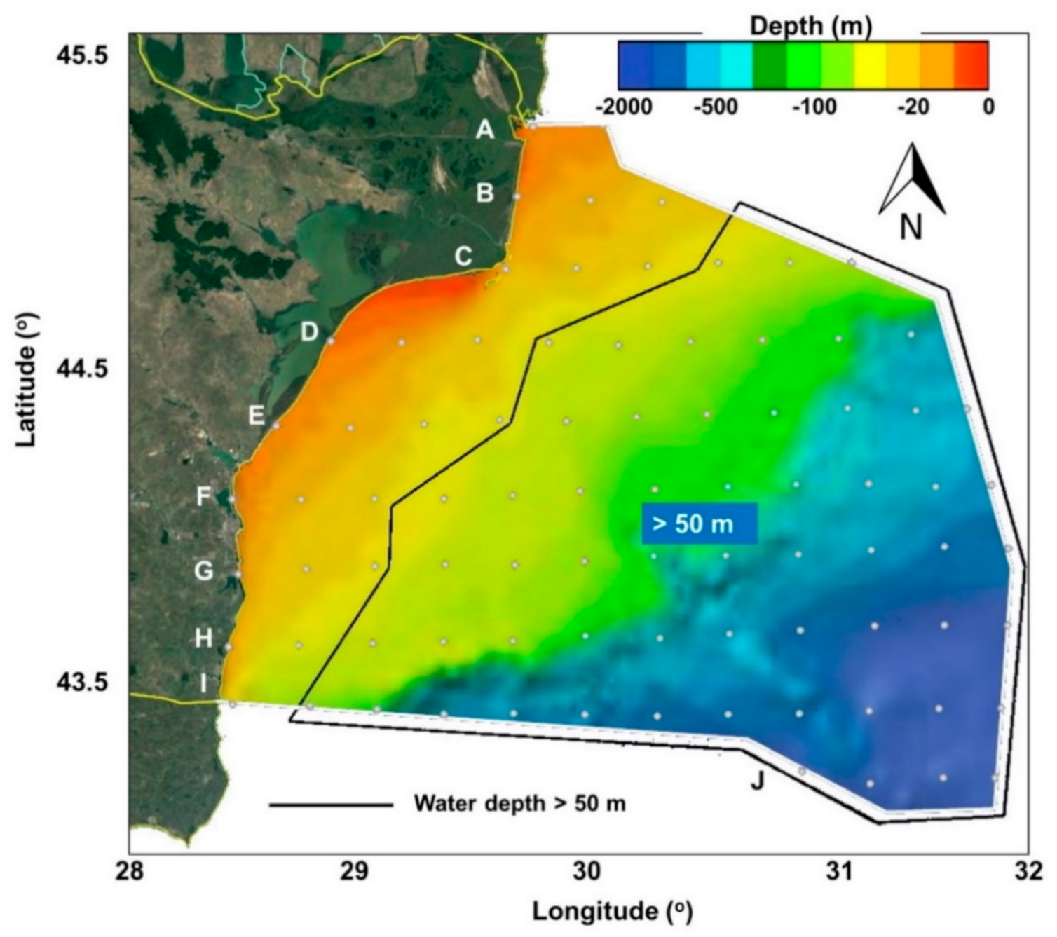
The first sector is more important from an ecological point of view, while the second is related to economical activities, such as ports, but also significant touristic activities. It is estimated that almost 4.50% of Romania’s population is located here, which per total covers a share of 5.30% from the entire Black Sea coastline [19]. Figure 1 presents the target area that is delimited by the EEZ borders, including the water depth details processed from GEBCO (general bathymetric chart of the oceans) [20]. The Romanian EEZ is delimited by the latitude lines 43.4398° N and 45.2128° N, while on the longitude the interval goes from 28.5278° E to 31.4097° E [21].
A total of 84 points were defined in a grid (lines from A to J), the distance between each point being constant, approximately 20 km along the x and y directions. In addition, a water depth of 50 m was considered as a reference, since this represents the threshold that separates the fixed offshore wind farms from the floating ones [22,23]. By considering these points it is possible to obtain a general picture of the energy potential and the performances of a particular turbine, which can be further extended to a more detailed investigation. As a limitation of this work, the restricted areas were not taken into account, but from the information provided by Văidianu and Ristea [19], we can notice that the entire water strip located close to the shore (<50 m) is defined by shipping activities, while on the north we notice some large protected areas. Figure 1 illustrates also the water depth, and we can notice that the points located close to the shore indicate values in the range 2–24 m. The values start to increase as we go further into the deeper sea, being expected for each step of 20 km (along x axis) an increase in the water depth by 10 m for each reference line until the 100 km limit, while after that the values jump to a maximum of 1747 m (line I—Vama Veche).
2.2. Wind Data
Two different datasets are considered in the present work. The first is related to ERA5 [24]. This is a state-of-the-art global atmospheric product delivered by the European Centre for Medium-Range Weather Forecasts (ECMWF), which includes multiple climate variables such as rainfall, land surface temperature or wind data over the ocean environment [25,26,27]. This dataset covers the interval from 1979 to the present and incorporates some new techniques such as the ECMWF Integrated Forecast System model (IFS 41r2). This update aimed to increase both the temporal output (to 24 values per day), and the horizontal and vertical resolutions (to 0.25° and 137 vertical levels starting from the surface to 0.01 hPa). Some other improvements were introduced, this being the case of a new data assimilation scheme or the update of the parametrization schemes. More details about this project are provided in Hersbach et al. [24], while some other relevant information related to the ERA5 wind data can be found in Soares et al. [28], Ulazia et al. [29] or Carreno-Madinabeitia et al. [30]. Table 1 presents the characteristics of the ERA5 data processed in the framework of this work, where the following two types of data are considered: (a) wind speed at 10 m height above the sea level (U10); and (b) wind speed at 100 m height (U100). These values are directly obtained from the ECMWF database, without any further adjustment. The second wind dataset comes from AVISO (archiving, validation and interpretation of satellite oceanographic) data, which is a project that combines multiple altimeter missions. The TOPEX/POSEIDON mission was initiated in 1992, being designed to measure the wind speed. Over time, some new missions were launched (Jason-3, Sentinel-3A, Saral, Cryosat-2, Jason-1&2, T/P, Envisat, GFO, ERS-1 & 2 and Geosat), so a consistent dataset was produced [31]. Most of the satellites were placed on near-polar or sun-synchronous orbits, being defined by nadir-looking instruments having a footprint of the beam of 10 km wide. Each mission is defined by a ground track separation that has an orbit geometry that can go up to 400 km at the equator, each satellite repeating the same ground track on an interval of 3 to 10 days [32]. In Table 1, more details regarding this dataset are provided.
2.3. Methods
The offshore wind industry is evolving very fast and at this moment it seems that there is interest in assessing the wind energy potential at a hub height of 100 m [28,33] and therefore the ERA5 (U100) wind dataset is a suitable candidate.
Going further from this, the annual electricity production (AEP) of a wind turbine, can be estimated as in Equation (1) [34]:
where AEP—in MWh; T—number of hours per year (8760 h/year); f(u)—Weibull distribution; P(u)—power curve of a turbine; and Cut-in/Cut-out—turbine characteristics.
The Weibull probability density function, can be defined as in Equation (2) [35]:
where u—the wind speed; k—the shape parameter; and c—the scale parameter (in m/s). Looking at some previous studies, we find that this method is not the most accurate one, since it may generate large uncertainties. For example, in the work of Elfarra and Kaya [36], two sites from the Aegean Sea and Mexico were evaluated, and it is noticed that for the sites located in the Mediterranean Sea the Weibull distribution overestimated the AEP by more than 10% while for the other site, the AEP production was underestimated by more than 6%. Also in the work of Jaramillo and Borja [37], it is mentioned that the AEP may be underestimated by at least 12%, which is caused mainly by the underestimation of the wind speeds from the intervals 12 and 20 m/s.
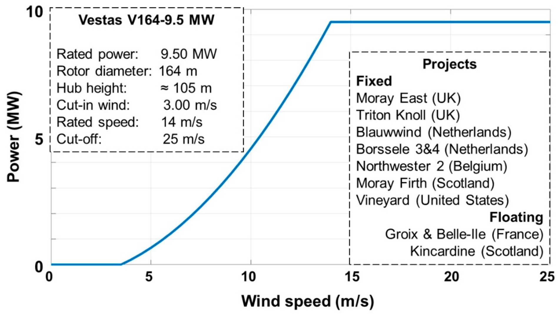
A single type of wind turbine will be considered for evaluation in this work. This is the Vestas V164-9.5 that is already implemented in various European offshore projects (fixed or floating). This is one of the largest wind generators available on the market (9.5 MW). Its performance will be evaluated at a hub height of 100 m. More details about this system and some of the related projects are provided in Figure 2.
3. Results
3.1. Comparisons between the Datasets
ERA5 is used as the main source of data in this work, and therefore it is important to understand the differences between some alternative data sources, in this case, AVISO. Figure 3 presents the distribution of the U10 values (50th and 95th percentiles) as provided by ERA5. For the 50th percentiles (50th), the wind speed is in the range 4.11–5.97 m/s for the points located at approximately 40–60 km from the shore, and this gradually expands to 6.09 m/s close to the extremity of the EEZ zone (in the south). Per total, the points located in the southern part (from line G down) seem to be a less attractive option since they are defined by a higher water depth and lower wind resources (e.g., 5.72 m/s—line J). However, the installation of floating wind turbines can be a viable solution in areas with depths that do not allow the installation of fixed turbines. As for the 95th percentiles, the maximum values are close to 11.50 m/s, corresponding mainly to the offshore sites. In contrast, the points located close to the shore indicate a maximum value of 9.93 m/s (Sacalin Peninsula—point C1). This clearly shows that the wind energy potential in the target area increases as we go from onshore to offshore, the most promising sites for developing a wind project being located along the C-line.
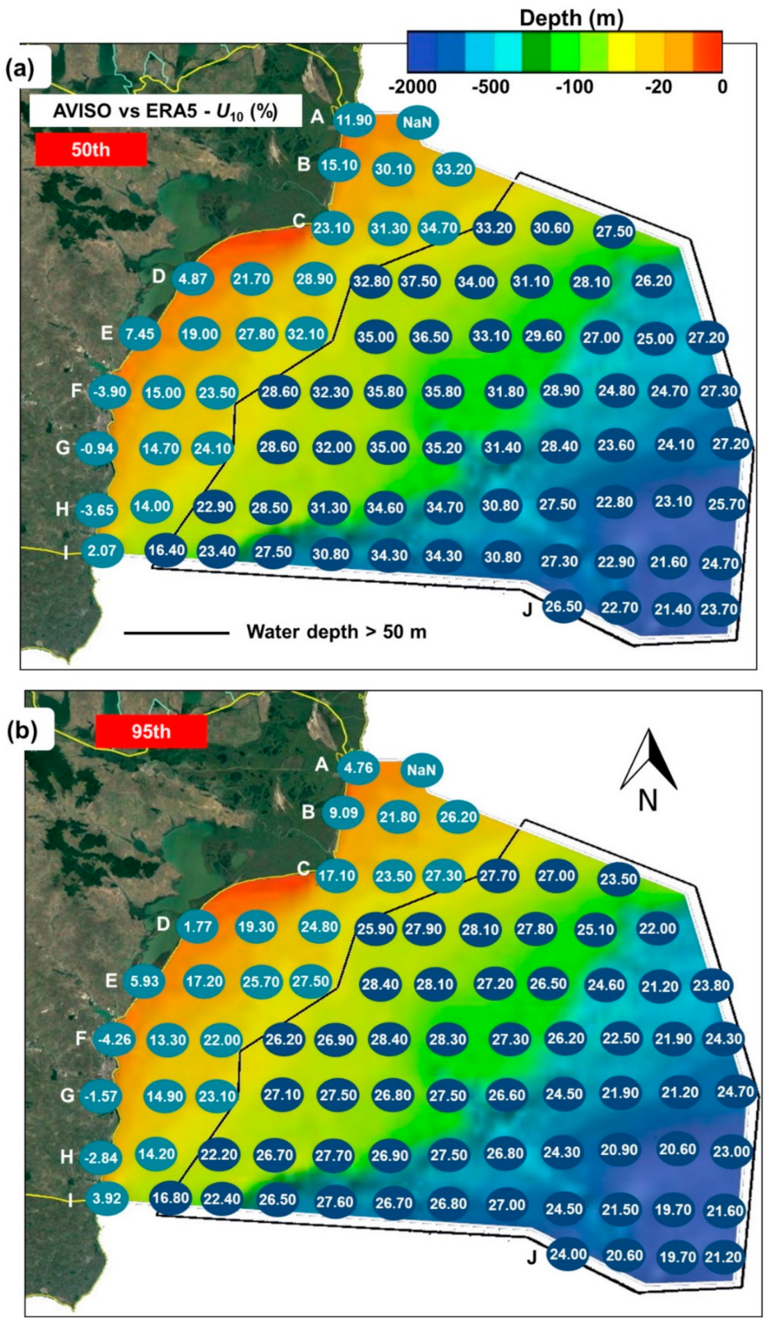
Figure 4 presents a direct comparison between the AVISO and ERA5 data (U10), where the results are expressed in percentages. The relative differences between ERA5 and AVISO are quantified as in Equation (3):
The daily average values of ERA5 U10 were computed in order to be compared with the daily mean values provided by AVISO. Excepting some points located close to the shore (lines F, G and H), all the values are positive which means that the ERA5 data indicate higher values than AVISO. A well-known issue related to the satellite measurements concerns the accuracy of the measurements on the land–sea interface, in this case being noticed as the NaN (not a number) values along the A-line. The NaN indicator is used to show that there are no valid data reported by the AVISO dataset. For the 50th percentiles (Figure 4a), the points located in the central and southern parts (close to the shore) show a better agreement, while the maximum differences of 36% occur in the center of the target area. These differences are better quantified in Table 2, where besides the 50th and 95th percentiles, the 25th and 75th percentiles are also computed, where for example D0 indicates a point located along the line D at 0.00 distance from the coast, while D80 is used to identify a similar point located at 80 km from the shore. For the 95th percentile, the best agreement corresponds to the nearshore points (1.57% and 4.26%), compared to some other points located at 80 or 120 km from the shore, where the differences reach 28.40%.
3.2. Assessment of the Wind Energy Potential
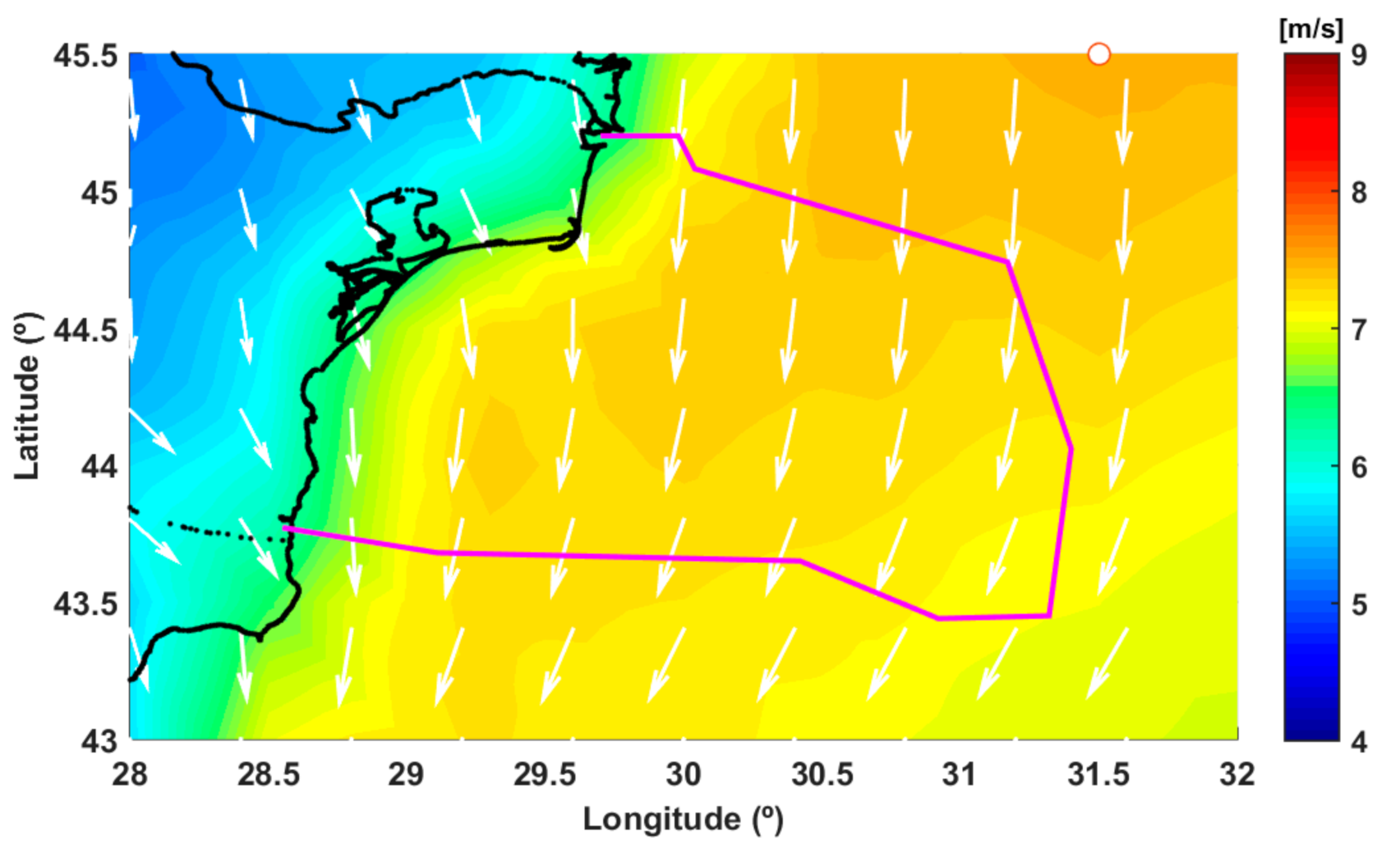
Figure 5 provides the first representation of the wind energy distribution over the Romanian coastal area, including also the land. The results clearly show that the wind speed increases from the land (~5.00 m/s) to the shoreline, and further to the offshore regions. Near the shoreline the values can go up to 6.00 m/s, while from the marine areas the northern part indicates higher values, reaching a maximum of 7.48 m/s outside the Romanian national waters (in the Ukrainian area). Regarding the wind direction, several patterns are noticed. For the wind fields over the land, the dominant direction is from the land to the sea (oriented to the southeast), while near the shoreline the wind usually follows the local coastline. As we go further offshore, the wind field starts to curve, being oriented to the southwest direction.
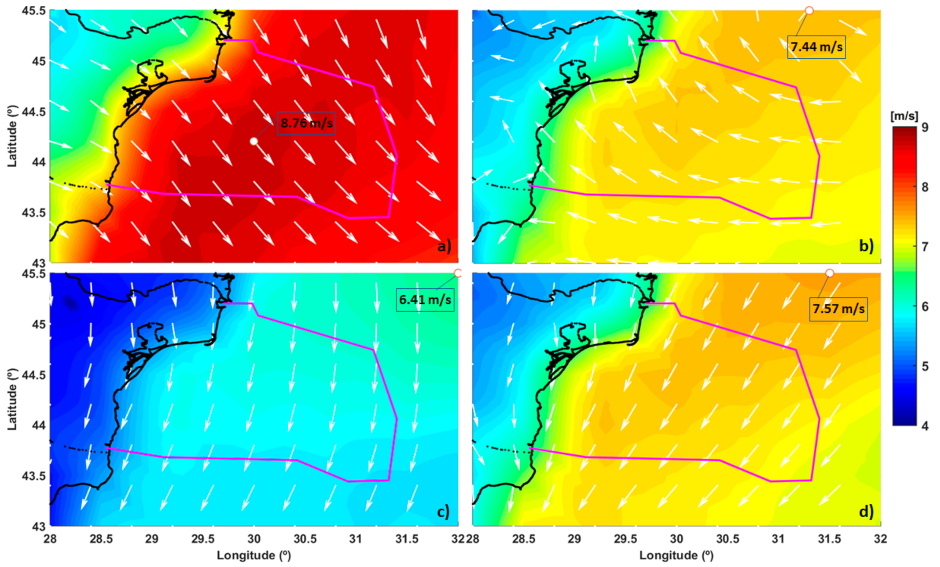
A similar analysis is presented in Figure 6, considering this time the seasonal distribution (spring–summer–autumn–winter) of the parameter U100. Regardless of the season, we notice that the wind conditions increase as we go from land to sea. The maximum values are located outside the Romanian coastal waters, excepting the wintertime when a maximum value of 8.76 m/s occurs in the center of the target area. This suggests that during the most energetic season (December–January–February), a wind project located in this area will obtain the best performances. More than this, the point indicated is located outside the restricted areas where the harbor activities usually take place [19], so this location may be considered a suitable candidate for a wind project. The summer season indicates lower resources, reaching a maximum value of 6.41 m/s, while the spring and autumn seasons are about the same level, reaching values of 7.44 and 7.57 m/s, respectively.
Regarding the wind directions, the patterns corresponding to the summer and autumn seasons are similar to the prevailing wind direction corresponding to the total time (Figure 5). In the case of spring, the dominant pattern is from sea to land (from east to west), being noticed close to the Danube Delta a tendency to shift in the northern sector. During the winter, the wind is moving to blow from the northwest and small changes in the orientation of the wind vectors are observed. The wind direction represents an important aspect of the design of a wind farm, considering that the energy produced is significantly affected by the wake effect. It is estimated that for the offshore projects, these losses are in the range 10.00–25.00% [40,41].
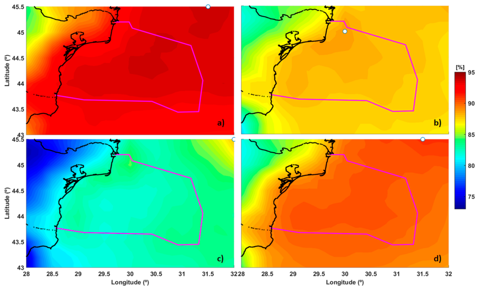
As mentioned above, wind turbines are designed to operate within a specific range of wind speeds, known as the cut-in and cut-out values. The turbine considered in this study has wind speed limits in the range of 3.00–25.00 m/s. That is why the percentages of U100 that were inside the functional range of the wind turbine were computed for each season, and the results are illustrated in Figure 7. It must be noticed that along the Romanian coast, percentages higher than 80% are observed in all seasons. As expected, percentages above 90% are found in the winter season.
An important role in choosing a location for exploiting wind energy is the variability of the wind speed over the years. The IAV (interannual variability) index is often used in climatologic analyses to quantify the year-to-year variability of a given parameter. This can be expressed as in Equation (4) [26,42]:
where IAV—inter-annual variability (%); x denotes the time series of the wind speed over a period of m years with n records each; —mean value of the time series of a parameter over a period of years; —standard deviation; the indices j and k refer to the year and record, respectively; and overbar denotes an average.
Thus, the year-to-year variability of U100 from the ERA5 database over the 20-year time interval 2000–2019 was quantified here and the results are illustrated in Figure 8. It can be observed that IAV increases as we move away from the shore. At this point, it has to be noticed that if for the coefficient of the variation in the wind speed there might be expected higher values on land than offshore, this inter-annual variability index shows very often higher values offshore, as can be noticed in the Figure 8 results which are also consistent with those presented in [42].
The capacity factor is frequently used to assess the performances of a wind turbine, this is defined as in Equation (5) [43]:
where Cf—capacity factor (%); —expected power to be generated by a turbine (MW); and —rated power of a turbine (9.50 MW from Figure 2).
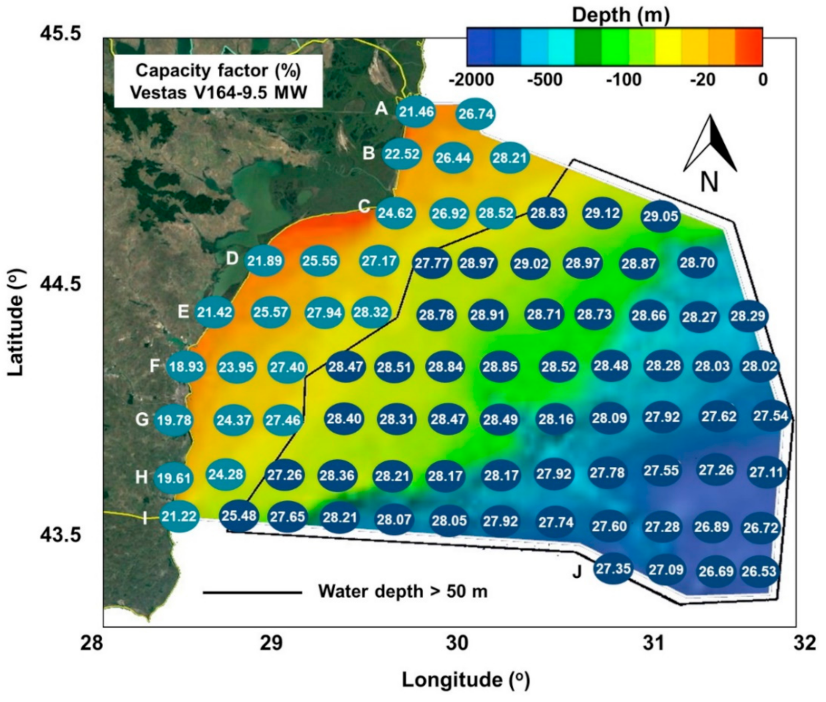
Figure 9 presents such an analysis considering the performances of the Vestas V164-9.5 wind turbine for the full-time distribution. Although the wind speed increases as we go further from the shore, this is not the case for the Cf indicator that for example indicates values of 28.50% for the point C40 (40.00 km from the shore), compared to values of 27.00% for the eastern boundary of EEZ. For this turbine a maximum value of 29.12% is observed near the point C80, being followed by C100 and D100/D120 with values close to 29.00%. From the points located close to the shoreline, better performances are expected for the Danube Delta (e.g., 24.62%), while from the southern part, the point I0 (Vama Veche) looks more promising with 21.22%. The points located near the interface that separates the shallow and deep waters (50 m) can be considered a promising candidate for a wind project since (a) they are defined by a higher Cf ~28.00%; (b) they are located close to the shore and in a lower water depth, which is in the line with the current European trends; and (c) it is possible to develop either fixed or floating projects.
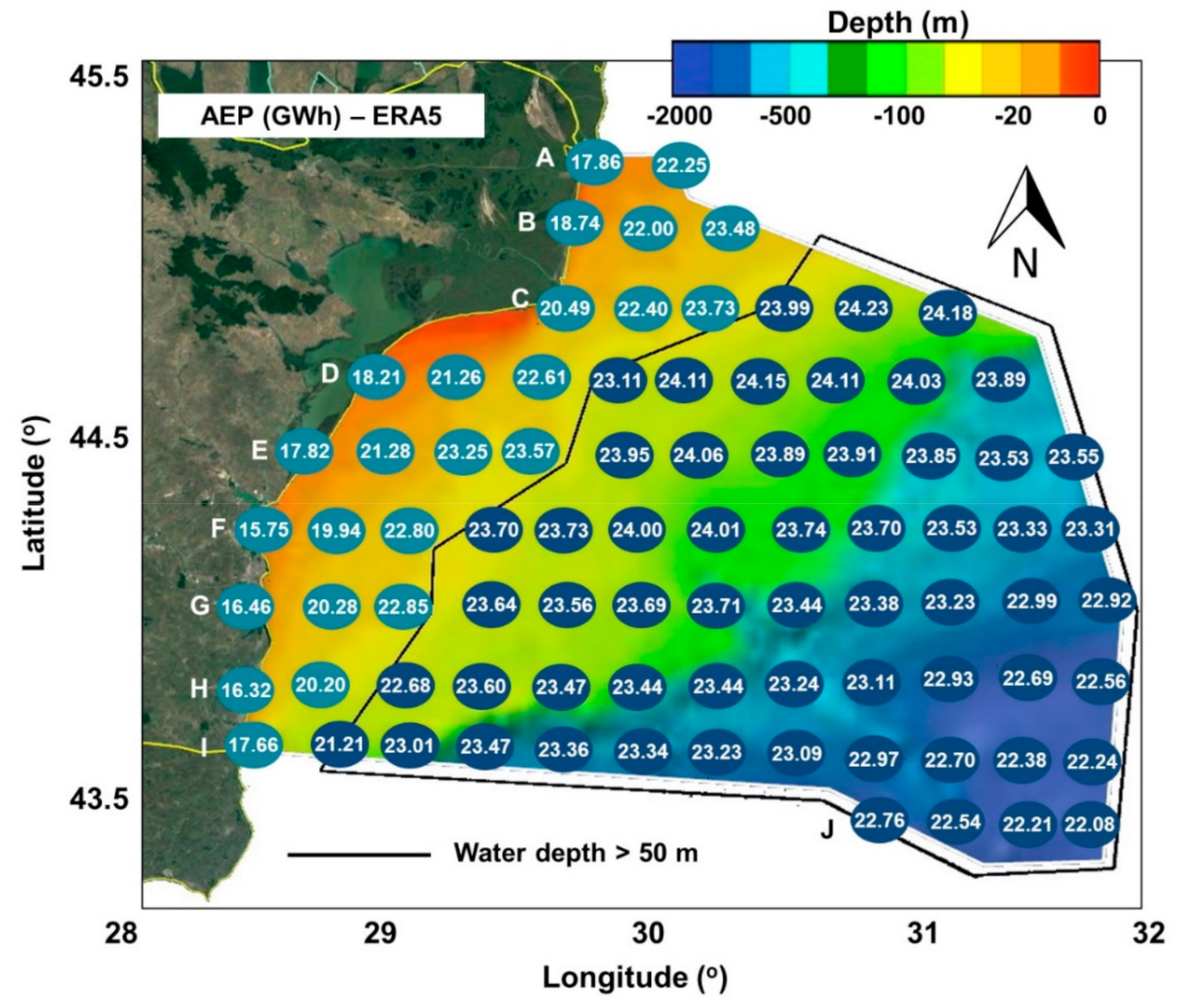
The annual energy production (GWh) is illustrated in Figure 10, these values correspond to a single wind turbine, Vestas V164-9.5, which may operate in a particular point of the grid. The top values are in the range 23.00–24.00 GWh, while a significant drop occurs near the shoreline to a minimum of 16.32 GWh (approximately a 35.00% difference), these values corresponding to the point H0. From the shallow–deep water interface, we can highlight the points C40 (23.73 GWh) and E60 (23.57 GWh), while from the offshore the C points located at the extremity of the EEZ indicate better results (e.g., C80—24.23 GWh).
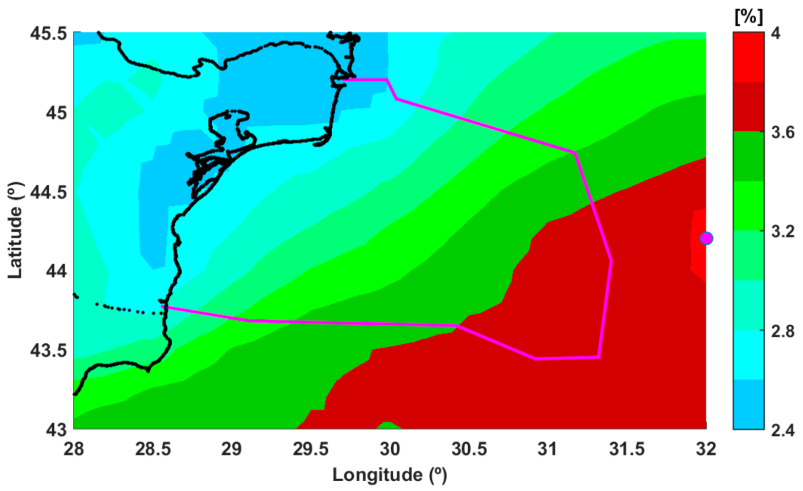
The IAV index is also used to assess the energy production of the turbine for this target area and the parameter analyzed over the 20 years is now AEP. In Figure 11 is provided such an analysis, by considering the ERA5 wind data. The IAV increases from the onshore to offshore areas, reaching a maximum value of 7.55% in the southeastern part of the target area. These values also increase from north to south, reaching a minimum of 5.56% close to the site A20, while near the shoreline the values go from 5.72% (A0) to 6.72% (I0). From all the sites, the J line indicates higher values (7.45 to 7.53%), a possible explanation being related to the distance from the shore (>120.00 km) or the water depth (>1200.00 m).
4. Discussion
A preliminary step in the development of a renewable project consists in the analysis of the environmental conditions, the reanalysis data being capable to provide a more complete picture of the wind conditions [44,45,46]. Compared to the general wind patterns in the Black Sea, the Romanian coastal region is defined by more consistent wind energy resources, at which we can add a lower water depth that is related to the continental shelf [47]. Furthermore, the structure of the local seabed in the upper layers is mostly made by sand and clay deposits [48], an aspect that needs to be considered in the selection of the right type of wind turbine foundation [49].
The results presented in this work are built around the ERA5 data, and from the analysis of the wind resources (U100) we notice that the wind speed increases from onshore to offshore, regardless of the time interval considered. These results are encouraging, taking also into account that near the Romanian coastline (on land) some important wind projects already operate successfully. The most representative example is the Fantanele-Cogealac wind farm (17.00 km from the Black Sea coast) that has an operational capacity of 600 MW. More than this, if we look at the wind farms of Romania, more than 78.00% of the projects are operating in the Dobrogea Plateau, which is next to the sea [50]. According to the IEC classification [51], the wind turbines from classes II and III are more suitable for this region, with better performances being expected during the wintertime when an average wind speed of 9.00 m/s is usually expected.
In relationship with some other works [15,16,52], this represents one of the first studies that evaluates the Romanian offshore wind energy potential using the new ERA5 data, which is defined by 24 values per day, and furthermore the evaluation is linked to a hub height of 100.00 m.
In the work of Cornett [53], several parameters are used to describe the temporal variability in the marine resources. One of them is the coefficient of variation (COV), which is defined as in Equation (6):
where σ is standard deviation; µ denotes the mean and the overbar is related to the time-averaging. A zero value of COV indicates that there is no variability, COV (U10) = 1 denotes that the standard deviation is equal to the mean value, while COV (U10) = 2 indicates that the standard deviation is twice the mean.
The seasonal variability (SV) is another indicator, which is defined as in Equation (7):
where U10S1 and U10S4 represent the mean wind speed being related to the most and least energetic seasons. In this case, winter (December–January–February) and summer (June–July–August) represent the two extreme seasons, the first being the most energetic. In the case of U10year, this was approximated as U10year ~ ½(U10S1 + U10S4), similar to the one mentioned by Cornett [53].
Table 3 shows the distribution of the COV values, considering the ERA5 wind dataset. In this case, the values increase from the nearshore points (0.46) to the offshore (0.50), being observed some values of 0.51 in the southern part. The SV indicator is presented in Table 4, where we can notice smaller differences. The values go from 0.30 to 0.41, much higher ones being found in the offshore area, especially for the sites located in the southern part.
Although the ERA5 data are frequently used to assess the renewable resources, due to the lower resolution of the global model it is possible that for some seas surrounded by complex orography (as for example is the Black Sea) underestimation of the wind speeds to occur. Consequently, such underestimations can propagate as regards the wind energy potential. The long-term variability in the resources estimated using COV and SV shows that ERA5 data indicate more stable conditions compared to the satellite measurements.
However, it has to be highlighted at this point that ERA5 U10 winds were verified by Belmonte and Stoffelen [54], showing rather large model errors near the coast. The model wind data do not appear very reliable in coastal areas, particularly for enclosed seas. This is probably due to the large diurnal cycle and the occurrence of low-level jets (LLJ), which are both not well captured by ERA5 [55]. On the other hand, the AVISO dataset is not a perfect daily mean, like the average of the 24 values for ERA5. In fact, altimeter winds over a day are determined by the local solar times of the contributing altimeter sample.
As the land–sea effects near the Romanian coast are substantial, the diurnal cycle will determine the mean daily wind. Hence, this AVISO product appears not suitable to verify the simulated gridded products. An altimeter does not measure the wind at a 10 m height, but rather the ocean roughness, which may be related to the 10 m stress-equivalent wind [56]. Furthermore, the altimeter speeds are sensitive to the mean squared slope (MSS) of the ocean, and hence sensitive to the sea state which may be quite detrimental for coastal validation. Some other limitations of the ERA5 data for the energy assessments in the coastal area are further presented in Belmonte and Stoffelen [54], and Kalverla [55].
Most of the reanalysis datasets are providing data at the standard height of 10 m, which is suitable for meteorological applications, but to translate these values to a hub height, an adjustment is required (e.g., logarithmic law, power law, etc). One element of innovation that defines the ERA5 data is that it directly provides wind data at a 100 m height, considering that this is a reference height for the offshore industry [28,57].
In the work of Onea et al. [18], a similar analysis was carried out for the Romanian EEZ, considering this time for evaluation an MHI Vestas V174 9.5 MW turbine. For the present work, we considered to use the V164-9.5 MW system since all the information needed to assemble the power curve is available in the public domain (e.g., rated wind speed), which is not the case for the other system [58]. The present turbine is defined by a lower capacity factor compared to the V174 9.5, which may reach a maximum of 35.00% in the upper part of the EEZ, which is up to 6.00% compared to the one presented in this study. The main explanation for this is related to the fact that the V174 9.5 wind turbine has a lower rated speed, which makes it more competitive. These values are relatively close to the capacity factor (36%) estimated for Romania and Bulgaria, exceeding those corresponding to countries such as Italy (25–30%), Greece (29%) or Spain (31%), but far under regions like the UK (53%) or Denmark (44%), where significant offshore projects already operate [59].
5. Conclusions
In the present work, an assessment of the wind energy potential was carried out in the Romanian EEZ, considering multiple datasets that cover a total of 20 years (2000–2019). Special attention was given to the ERA5 data since these are frequently used for renewable applications. The results clearly show an increase in the wind conditions as going from the land to the sea, which means that an offshore project could become a reality in this coastal environment in the near future.
During the more energetic seasons, the average wind speed can frequently reach 8–9 m/s, values that are related to the IEC classes II and III. Taking also into account the fact that in the southern part of the Romanian nearshore some important seaports are located (for example Constanta harbor), this means that the logistic support required to develop a wind project will be more accessible. On the other hand, higher wind resources are characteristic in the northern part of the target area, where the capacity factor of the wind turbine considered for evaluation (V164-9.5 MW) frequently indicates a value of about 30%.
From this perspective, it can be concluded that the Romanian offshore wind sector represents a viable alternative to the Romanian coal power plants that during recent years gradually reduced their production capacity. The present work also opens some new research ideas that need to be tackled soon, such as the assessment of the wind energy potential by considering restricted areas, and to identify suitable wind farm layouts and consider the fluctuations in the wind direction.
Per total, the Romanian coastal area can be considered a viable candidate for the development of an offshore wind project having good wind energy potential, a large continental shelf, and also Romania is a part of the European Union that aims to significantly expand the offshore wind sector. It can be also highlighted that various projects are targeting the development of offshore wind farms very soon in this particular coastal environment, and for them the present study should be of great interest. The western part of the Black Sea has important wind resources that need to be accurately quantified to establish the expected performances of the offshore wind turbines. The first step is to understand the limitations of the global reanalysis dataset and of the satellite measurements, by making a direct comparison with in situ measurements. Regarding the Romanian EEZ, it is expected that in future works we will also include some restricted areas (e.g., shipping routes, protected areas), in order to identify the most suitable areas capable to support a marine project. Finally, it is important to mention also that at this moment the ERA5 wind data are capable to provide a general perspective of the wind conditions over a long time interval, being processed on a global scale. Nevertheless, there are now some other wind datasets available with a higher resolution, which include meso- and micro-scaling that can be used to evaluate the wind resources in the coastal environment. This is the case of the Global Wind Atlas [60] that is defined by a grid spacing of 3 km. For regional simulations, the ERA5 boundary conditions are used to force the mesoscale model, but at this moment the data available cover only the 10-year time interval 2008–2017. The present work is ongoing and this type of data represents a valuable tool for the assessment of the sites located near the coastline or onshore, where the topographic details become more important in wind modelling. At this point it has to be also highlighted that aspects of space and time sampling are relevant for observations, while they provide the only absolute source of wind information. Model winds are affected by simulation artefacts, such as varying observation input over time, diffusion of land–sea effects, diurnal cycle, convection, etc. Extensive inter-calibrated and documented satellite records of winds are publicly available in the EU Copernicus Marine Environment Monitoring Service, but not considered in the present work. From this perspective, an important objective of the future work is to complete the study related to the assessment of the offshore wind energy potential in the Romanian exclusive economic zone with an extended analysis of these scatterometer winds.
Author Contributions
F.O. performed the literature review, processed the data, and wrote the manuscript. E.R. designed and supervised the present work. L.R. contributed to the design and implementation of the research. All authors have read and agreed to the published version of the manuscript.
Funding
This work was carried out in the framework of the research project DREAM (Dynamics of the REsources and technological Advance in harvesting Marine renewable energy), supported by the Romanian Executive Agency for Higher Education, Research, Development and Innovation Funding—UEFISCDI, grant number PN-III-P4-ID-PCE-2020-0008.
Acknowledgments
The data used in this study are openly available. ERA5 data used in this study were obtained from the ECMWF data server. The altimeter products were generated and distributed by AVISO (http://www.aviso.altimetry.fr/, accessed on 29 March 2021) as part of the Ssalto ground processing segment.
Conflicts of Interest
The authors declare no conflict of interest.
References
- Ahmad, T.; Zhang, D. A Critical Review of Comparative Global Historical Energy Consumption and Future Demand: The Story Told so Far. Energy Rep. 2020, 6, 1973–1991. [Google Scholar] [CrossRef]
- Kesicki, F.; Anandarajah, G. The Role of Energy-Service Demand Reduction in Global Climate Change Mitigation: Combining Energy Modelling and Decomposition Analysis. Energy Policy 2011, 39, 7224–7233. [Google Scholar] [CrossRef]
- Brockway, P.E.; Sorrell, S.; Semieniuk, G.; Heun, M.K.; Court, V. Energy Efficiency and Economy-Wide Rebound Effects: A Review of the Evidence and Its Implications. Renew. Sustain. Energy Rev. 2021, 141, 110781. [Google Scholar] [CrossRef]
- Erdiwansyah; Mahidin; Mamat, R.; Sani, M.S.M.; Khoerunnisa, F.; Kadarohman, A. Target and Demand for Renewable Energy across 10 ASEAN Countries by 2040. Electr. J. 2019, 32, 106670. [Google Scholar] [CrossRef]
- Brugger, H.; Eichhammer, W.; Mikova, N.; Dönitz, E. Energy Efficiency Vision 2050: How Will New Societal Trends Influence Future Energy Demand in the European Countries? Energy Policy 2021, 152, 112216. [Google Scholar] [CrossRef]
- Elrahmani, A.; Hannun, J.; Eljack, F.; Kazi, M.-K. Status of Renewable Energy in the GCC Region and Future Opportunities. Curr. Opin. Chem. Eng. 2021, 31, 100664. [Google Scholar] [CrossRef]
- Cheng, K.-S.; Ho, C.-Y.; Teng, J.-H. Wind Characteristics in the Taiwan Strait: A Case Study of the First Offshore Wind Farm in Taiwan. Energies 2020, 13, 6492. [Google Scholar] [CrossRef]
- Cottura, L.; Caradonna, R.; Ghigo, A.; Novo, R.; Bracco, G.; Mattiazzo, G. Dynamic Modeling of an Offshore Floating Wind Turbine for Application in the Mediterranean Sea. Energies 2021, 14, 248. [Google Scholar] [CrossRef]
- Costa, Á.M.; Orosa, J.A.; Vergara, D.; Fernández-Arias, P. New Tendencies in Wind Energy Operation and Maintenance. Appl. Sci. 2021, 11, 1386. [Google Scholar] [CrossRef]
- Offshore Wind in Europe—Key Trends and Statistics 2020. Available online: https://windeurope.org/data-and-analysis/product/offshore-wind-in-europe-key-trends-and-statistics-2020 (accessed on 11 March 2021).
- Topham, E.; McMillan, D.; Bradley, S.; Hart, E. Recycling Offshore Wind Farms at Decommissioning Stage. Energy Policy 2019, 129, 698–709. [Google Scholar] [CrossRef] [Green Version]
- Onea, F.; Rusu, L. A Long-Term Assessment of the Black Sea Wave Climate. Sustainability 2017, 9, 1875. [Google Scholar] [CrossRef] [Green Version]
- Onea, F.; Rusu, E. Sustainability of the Reanalysis Databases in Predicting the Wind and Wave Power along the European Coasts. Sustainability 2018, 10, 193. [Google Scholar] [CrossRef] [Green Version]
- Pasimeni, F.; Fiorini, A.; Georgakaki, A. Assessing Private R&D Spending in Europe for Climate Change Mitigation Technologies via Patent Data. World Pat. Inf. 2019, 59, 101927. [Google Scholar] [CrossRef]
- Onea, F.; Rusu, L. Evaluation of Some State-Of-The-Art Wind Technologies in the Nearshore of the Black Sea. Energies 2018, 11, 2452. [Google Scholar] [CrossRef] [Green Version]
- Onea, F.; Rusu, L. A Study on the Wind Energy Potential in the Romanian Coastal Environment. J. Mar. Sci. Eng. 2019, 7, 142. [Google Scholar] [CrossRef] [Green Version]
- Rusu, E. A 30-Year Projection of the Future Wind Energy Resources in the Coastal Environment of the Black Sea. Renew. Energy 2019, 139, 228–234. [Google Scholar] [CrossRef]
- Romania’s Offshore Wind Energy Resources: Natural Potential, Regulatory Framework, and Development Prospects; EPG: Bucharest, Romania, 2020.
- Văidianu, N.; Ristea, M. Marine Spatial Planning in Romania: State of the Art and Evidence from Stakeholders. Ocean Coast. Manag. 2018, 166, 52–61. [Google Scholar] [CrossRef] [Green Version]
- GEBCO_08 Grid—Version 20100927. Available online: https://www.gebco.net/data_and_products/gridded_bathymetry_data/version_20100927/ (accessed on 25 April 2021).
- Flanders Marine Institute (VLIZ). Belgium Maritime Boundaries Geodatabase: Maritime Boundaries and Exclusive Economic Zones (200NM); Flanders Marine Institute: Ostend, Belgium, 2019. [Google Scholar]
- Lin, Z.; Liu, X.; Lotfian, S. Impacts of Water Depth Increase on Offshore Floating Wind Turbine Dynamics. Ocean Eng. 2021, 224, 108697. [Google Scholar] [CrossRef]
- Díaz, H.; Guedes Soares, C. Review of the Current Status, Technology and Future Trends of Offshore Wind Farms. Ocean Eng. 2020, 209, 107381. [Google Scholar] [CrossRef]
- Hersbach, H.; Bell, B.; Berrisford, P.; Hirahara, S.; Horányi, A.; Muñoz-Sabater, J.; Nicolas, J.; Peubey, C.; Radu, R.; Schepers, D.; et al. The ERA5 Global Reanalysis. QJR Meteorol. Soc. 2020, qj.3803. [Google Scholar] [CrossRef]
- Onea, F.; Rusu, L.; Carp, G.B.; Rusu, E. Wave Farms Impact on the Coastal Processes—A Case Study Area in the Portuguese Nearshore. J. Mar. Sci. Eng. 2021, 9, 262. [Google Scholar] [CrossRef]
- Rusu, L.; Rusu, E. Evaluation of the Worldwide Wave Energy Distribution Based on ERA5 Data and Altimeter Measurements. Energies 2021, 14, 394. [Google Scholar] [CrossRef]
- Olauson, J. ERA5: The New Champion of Wind Power Modelling? Renew. Energy 2018, 126, 322–331. [Google Scholar] [CrossRef] [Green Version]
- Soares, P.M.M.; Lima, D.C.A.; Nogueira, M. Global Offshore Wind Energy Resources Using the New ERA-5 Reanalysis. Environ. Res. Lett. 2020, 15, 1040a2. [Google Scholar] [CrossRef]
- Ulazia, A.; Sáenz, J.; Ibarra-Berastegi, G.; González-Rojí, S.J.; Carreno-Madinabeitia, S. Global Estimations of Wind Energy Potential Considering Seasonal Air Density Changes. Energy 2019, 187, 115938. [Google Scholar] [CrossRef]
- Carreno-Madinabeitia, S.; Ibarra-Berastegi, G.; Sáenz, J.; Ulazia, A. Long-Term Changes in Offshore Wind Power Density and Wind Turbine Capacity Factor in the Iberian Peninsula (1900 to 2010). Energy 2021, 120364. [Google Scholar] [CrossRef]
- Home: Aviso+. Available online: https://www.aviso.altimetry.fr/en/home.html (accessed on 31 May 2019).
- Ribal, A.; Young, I.R. 33 Years of Globally Calibrated Wave Height and Wind Speed Data Based on Altimeter Observations. Sci Data 2019, 6, 77. [Google Scholar] [CrossRef] [Green Version]
- Majidi Nezhad, M.; Shaik, R.U.; Heydari, A.; Razmjoo, A.; Arslan, N.; Astiaso Garcia, D. A SWOT Analysis for Offshore Wind Energy Assessment Using Remote-Sensing Potential. Appl. Sci. 2020, 10, 6398. [Google Scholar] [CrossRef]
- Rusu, E.; Onea, F. An Assessment of the Wind and Wave Power Potential in the Island Environment. Energy 2019, 175, 830–846. [Google Scholar] [CrossRef]
- Salvação, N.; Guedes Soares, C. Wind Resource Assessment Offshore the Atlantic Iberian Coast with the WRF Model. Energy 2018, 145, 276–287. [Google Scholar] [CrossRef]
- Ali Elfarra, M.; Kaya, M. Estimation of Electricity Cost of Wind Energy Using Monte Carlo Simulations Based on Nonparametric and Parametric Probability Density Functions. Alex. Eng. J. 2021, 60, 3631–3640. [Google Scholar] [CrossRef]
- Jaramillo, O.A.; Borja, M.A. Wind Speed Analysis in La Ventosa, Mexico: A Bimodal Probability Distribution Case. Renew. Energy 2004, 29, 1613–1630. [Google Scholar] [CrossRef]
- V-V164-9.5 MWTM. Available online: https://www.vestas.com/en/products/offshore platforms/v164_9_5_mw (accessed on 21 March 2021).
- MHI Vestas Offshore V164/9500—Manufacturers and Turbines—Online Access—The Wind Power. Available online: https://www.thewindpower.net/turbine_en_1476_mhi-vestas-offshore_v164-9500.php (accessed on 19 August 2018).
- Xie, K.; Yang, H.; Hu, B.; Li, C. Optimal Layout of a Wind Farm Considering Multiple Wind Directions. In Proceedings of the 2014 International Conference on Probabilistic Methods Applied to Power Systems (PMAPS); IEEE: Durham, UK, 2014; pp. 1–6. [Google Scholar]
- Wu, Y.-T.; Porté-Agel, F. Modeling Turbine Wakes and Power Losses within a Wind Farm Using LES: An Application to the Horns Rev Offshore Wind Farm. Renew. Energy 2015, 75, 945–955. [Google Scholar] [CrossRef]
- Stopa, J.E.; Cheung, K.F.; Tolman, H.L.; Chawla, A. Patterns and Cycles in the Climate Forecast System Reanalysis Wind and Wave Data. Ocean Model. 2013, 70, 207–220. [Google Scholar] [CrossRef]
- Rusu, E.; Onea, F. A Parallel Evaluation of the Wind and Wave Energy Resources along the Latin American and European Coastal Environments. Renew. Energy 2019. [Google Scholar] [CrossRef]
- Kamranzad, B.; Etemad-Shahidi, A.; Chegini, V. Sustainability of Wave Energy Resources in Southern Caspian Sea. Energy 2016, 97, 549–559. [Google Scholar] [CrossRef] [Green Version]
- Lavidas, G.; Blok, K. Shifting Wave Energy Perceptions: The Case for Wave Energy Converter (WEC) Feasibility at Milder Resources. Renew. Energy 2021, 170, 1143–1155. [Google Scholar] [CrossRef]
- Jourdier, B. Evaluation of ERA5, MERRA-2, COSMO-REA6, NEWA and AROME to Simulate Wind Power Production over France. Adv. Sci. Res. 2020, 17, 63–77. [Google Scholar] [CrossRef]
- Onea, F.; Rusu, E. Wind Energy Assessments along the Black Sea Basin. Meteorol. Appl. 2014, 21, 316–329. [Google Scholar] [CrossRef]
- Dinu, C.; Wong, H.K.; Tambrea, D.; Matenco, L. Stratigraphic and Structural Characteristics of the Romanian Black Sea Shelf. Tectonophysics 2005, 410, 417–435. [Google Scholar] [CrossRef]
- Sánchez, S.; López-Gutiérrez, J.-S.; Negro, V.; Esteban, M.D. Foundations in Offshore Wind Farms: Evolution, Characteristics and Range of Use. Analysis of Main Dimensional Parameters in Monopile Foundations. J. Mar. Sci. Eng. 2019, 7, 441. [Google Scholar] [CrossRef] [Green Version]
- Dragomir, G.; Șerban, A.; Năstase, G.; Brezeanu, A.I. Wind Energy in Romania: A Review from 2009 to 2016. Renew. Sustain. Energy Rev. 2016, 64, 129–143. [Google Scholar] [CrossRef]
- Roach, S.; Park, S.M.; Gaertner, E.; Manwell, J.; Lackner, M. Application of the New IEC International Design Standard for Offshore Wind Turbines to a Reference Site in the Massachusetts Offshore Wind Energy Area. J. Phys. Conf. Ser. 2020, 1452, 012038. [Google Scholar] [CrossRef]
- Raileanu, A.B.; Onea, F.; Rusu, E. Implementation of Offshore Wind Turbines to Reduce Air Pollution in Coastal Areas—Case Study Constanta Harbour in the Black Sea. J. Mar. Sci. Eng. 2020, 8, 550. [Google Scholar] [CrossRef]
- Cornett, A.M. A Global Wave Energy Resource Assessment. In Proceedings of the Eighteenth (2008) International Offshore and Polar Engineering Conference; Chung, J.S., Ed.; International Society Offshore & Polar Engineers: Cupertino, CA, USA, 2008; Volume 1, pp. 318–326. ISBN 978-1-880653-70-8. [Google Scholar]
- Belmonte Rivas, M.; Stoffelen, A. Characterizing ERA-Interim and ERA5 Surface Wind Biases Using ASCAT. Ocean Sci. 2019, 15, 831–852. [Google Scholar] [CrossRef] [Green Version]
- Kalverla, P.C.; Holtslag, A.A.M.; Ronda, R.J.; Steeneveld, G.-J. Quality of Wind Characteristics in Recent Wind Atlases over the North Sea. Q. J. R. Meteorol. Soc. 2020, 146, 1498–1515. [Google Scholar] [CrossRef]
- de Kloe, J.; Stoffelen, A.; Verhoef, A. Improved Use of Scatterometer Measurements by Using Stress-Equivalent Reference Winds. Ieee J. Sel. Top. Appl. Earth Obs. Remote Sens. 2017, 10, 2340–2347. [Google Scholar] [CrossRef]
- ERA5: How Are the 100m Winds Calculated?—Copernicus User Support Forum—ECMWF Confluence Wiki. Available online: https://confluence.ecmwf.int/pages/viewpage.action?pageId=155343870 (accessed on 30 September 2020).
- Bauer, L. MHI Vestas Offshore V174-9.5—9,50 MW—Wind Turbine. Available online: https://en.wind-turbine-models.com/turbines/2138-mhi-vestas-offshore-v174-9.5 (accessed on 25 March 2021).
- European Commission Joint Research Centre. Wind Potentials for EU and Neighbouring Countries: Input Datasets for the JRC EU TIMES Model; Publications Office: Brussels, Belgium, 2018. [Google Scholar]
- Global Wind Atlas. Available online: https://globalwindatlas.info (accessed on 26 April 2021).
Figure 1.
Representation of the Romanian exclusive economic zone (EEZ) considering the spatial map and the grid points defined. The horizontal reference lines (denoted from A to J from north to south) include points distributed along a grid defined by an approximate length of 20 km (along x and y directions).

Figure 2.
Power curve of the Vestas V164-9.5 turbine, including some technical data (left side) and planned offshore wind projects (right side) [38,39].

Figure 3.
Percentiles distribution corresponding to the ERA5 (U10) reanalysis data for the 20-year time interval 2000–2019. The results are indicated in terms of: (a) 50th percentile; and (b) 95th percentile.
Figure 3.
Percentiles distribution corresponding to the ERA5 (U10) reanalysis data for the 20-year time interval 2000–2019. The results are indicated in terms of: (a) 50th percentile; and (b) 95th percentile.

Figure 4.
Comparisons between the AVISO (U10) measurements and the ERA5 (U10) reanalysis data for the 7-year time interval 2013–2019. The results are indicated in terms of: (a) 50th percentiles; (b) and 95th percentiles. A positive value indicates that the ERA5 wind speed is higher than that provided by the AVISO data.

Figure 5.
Average wind speed computed based on the ERA5 (U100) dataset for the Romanian coastal area over the time interval 2000–2019 (full-time distribution). The wind direction is represented by arrows, while the point defined by the highest wind speed is indicated with a white circle. The Romanian EEZ is indicated by the magenta line.

Figure 6.
The seasonal averaged wind speed as indicated by the ERA5 (U100) dataset for the Romanian coastal area over the time interval 2000–2019. Data corresponding to the following seasons are presented: (a) winter—December–January–February; (b) spring—March–April–May; (c) summer—June–July–August; and (d) autumn—September–October–November. The results include the wind direction vectors and the locations of the maximum wind speed, while the Romanian EEZ is indicated by the magenta line.

Figure 7.
Seasonal percentages of the wind speed (U100) in the range between the cut-in and cut-off values (standard functional range 3–25 m/s): (a) winter—December–January–February; (b) spring—March–April–May; (c) summer—June–July–August; and (d) autumn—September–October–November. The locations of the maximum values are marked by white circles, while the Romanian EEZ is indicated by the magenta line.

Figure 8.
Interannual variability (IAV) of U100 from ERA5, where the Romanian EEZ is indicated by the magenta line.
Figure 8.
Interannual variability (IAV) of U100 from ERA5, where the Romanian EEZ is indicated by the magenta line.

Figure 9.
Capacity factor (%) of the Vestas V164-9.5 turbine for the total time, corresponding to the grid points located inside the Romanian EEZ. The results are evaluated at a hub height of 100 m, for the time interval 2000–2019, by processing the ERA5 (U100) data.
Figure 9.
Capacity factor (%) of the Vestas V164-9.5 turbine for the total time, corresponding to the grid points located inside the Romanian EEZ. The results are evaluated at a hub height of 100 m, for the time interval 2000–2019, by processing the ERA5 (U100) data.

Figure 10.
Vestas V164-9.5—annual energy production (in GWh) computed for the total time interval considering the ERA5 (U100) reanalysis data.
Figure 10.
Vestas V164-9.5—annual energy production (in GWh) computed for the total time interval considering the ERA5 (U100) reanalysis data.

Figure 11.
Inter-annual variability (IAV) in the annual energy production for the Vestas V164-9.5 wind turbine. The results are computed for the total time interval considering the ERA5 (U100) reanalysis data.
Figure 11.
Inter-annual variability (IAV) in the annual energy production for the Vestas V164-9.5 wind turbine. The results are computed for the total time interval considering the ERA5 (U100) reanalysis data.


Table 1.
Characteristics of the datasets processed for assessing the wind conditions in the Romanian coastal area.
Table 1.
Characteristics of the datasets processed for assessing the wind conditions in the Romanian coastal area.
| Organization | ERA5 | AVISO |
|---|---|---|
| ECMWF | Archiving, Validation and Interpretation of Oceanographic Satellite Data | |
| Type | Reanalysis data | Satellite measurements |
| Spatial coverage | Global | Global |
| Horizontal resolution | 0.25° × 0.25° | 1.00° × 1.00° |
| Reference height (m) | 10, 100 | 10 |
| Time interval | 2000–2019 | 2013–2019 |
| Time resolution | 24 data per day | 1 value per day (daily mean value) |
Table 2.
Percentile comparisons between AVISO and ERA5 wind speeds at 10 m height above the sea level. The wind data are processed for the 7-year time interval 2013–2019, and a positive value indicates that the ERA5 wind speed is higher than that provided by AVISO.
Table 2.
Percentile comparisons between AVISO and ERA5 wind speeds at 10 m height above the sea level. The wind data are processed for the 7-year time interval 2013–2019, and a positive value indicates that the ERA5 wind speed is higher than that provided by AVISO.
| Percentile Differences (in %) | ERA5 (U10)–AVISO (U10) | |||||||||
|---|---|---|---|---|---|---|---|---|---|---|
| Top 5—Best Agreement Value (Reference Point) | Top 5—Lowest Agreement Value (Reference Point) | |||||||||
| 25th | −0.31 (D0) | 3.95 (E0) | −4.39 (I0) | −5.44 (G0) | −8.04 (F0) | 38.10 (D80) | 36.40 (E100) | 35.90 (F100) | 35.60 (G100) | 35.50 (F120) |
| 50th | −0.94 (G0) | 2.07 (I0) | −3.65 (H0) | −3.90 (F0) | 4.87 (D0) | 37.50 (D80) | 36.50 (E100) | 35.80 (F100) | 35.20 (G120) | 35.00 (E80) |
| 75th | −0.87 (D0) | −2.68 (H0) | 3.85 (I0) | −4.17 (F0) | 4.57 (D0) | 33.50 (D80) | 33.10 (E100) | 32.90 (F120) | 32.50 (E80) | 32.30 (G120) |
| 95th | −1.57 (G0) | 1.77 (D0) | −2.84 (H0) | 3.92 (I0) | −4.26 (F0) | 28.40 (E80) | 28.10 (D100) | 27.90 (D80) | 27.80 (D120) | 27.70 (H80) |
Table 3.
Distribution of the COV values indicated for the ERA5 data (U100), considering the time interval 2000–2019.
Table 3.
Distribution of the COV values indicated for the ERA5 data (U100), considering the time interval 2000–2019.
| Line | Distance to Shore (km) | |||||||||||
|---|---|---|---|---|---|---|---|---|---|---|---|---|
| 0 | 20 | 40 | 60 | 80 | 100 | 120 | 140 | 160 | 180 | 200 | 220 | |
| A | 0.47 | |||||||||||
| B | 0.47 | 0.48 | 0.49 | |||||||||
| C | 0.48 | 0.49 | 0.49 | 0.50 | 0.50 | 0.50 | ||||||
| D | 0.47 | 0.49 | 0.49 | 0.50 | 0.50 | 0.50 | 0.50 | 0.50 | 0.50 | |||
| E | 0.47 | 0.49 | 0.50 | 0.50 | 0.50 | 0.50 | 0.50 | 0.50 | 0.50 | 0.50 | 0.50 | |
| F | 0.46 | 0.48 | 0.50 | 0.50 | 0.50 | 0.50 | 0.50 | 0.50 | 0.50 | 0.50 | 0.50 | 0.50 |
| G | 0.46 | 0.48 | 0.50 | 0.51 | 0.50 | 0.50 | 0.50 | 0.50 | 0.50 | 0.50 | 0.50 | 0.50 |
| H | 0.46 | 0.49 | 0.50 | 0.51 | 0.51 | 0.51 | 0.51 | 0.50 | 0.50 | 0.50 | 0.50 | 0.50 |
| I | 0.47 | 0.50 | 0.51 | 0.51 | 0.51 | 0.51 | 0.51 | 0.51 | 0.50 | 0.50 | 0.50 | 0.50 |
| J | 0.50 | 0.50 | 0.50 | 0.50 | ||||||||
Table 4.
Distribution of the SV values indicated for the ERA5 data (U100), considering the time interval 2000–2019.
Table 4.
Distribution of the SV values indicated for the ERA5 data (U100), considering the time interval 2000–2019.
| Line | Distance to Shore (km) | |||||||||||
|---|---|---|---|---|---|---|---|---|---|---|---|---|
| 0 | 20 | 40 | 60 | 80 | 100 | 120 | 140 | 160 | 180 | 200 | 220 | |
| A | 0.30 | 0.32 | ||||||||||
| B | 0.32 | 0.33 | 0.34 | |||||||||
| C | 0.34 | 0.35 | 0.35 | 0.36 | 0.36 | 0.35 | ||||||
| D | 0.33 | 0.34 | 0.35 | 0.36 | 0.37 | 0.37 | 0.37 | 0.36 | 0.36 | |||
| E | 0.34 | 0.35 | 0.37 | 0.38 | 0.38 | 0.38 | 0.38 | 0.37 | 0.37 | 0.36 | 0.36 | |
| F | 0.33 | 0.35 | 0.37 | 0.38 | 0.39 | 0.39 | 0.39 | 0.38 | 0.38 | 0.38 | 0.37 | 0.36 |
| G | 0.34 | 0.36 | 0.38 | 0.39 | 0.39 | 0.39 | 0.39 | 0.39 | 0.39 | 0.38 | 0.38 | 0.37 |
| H | 0.35 | 0.37 | 0.38 | 0.40 | 0.40 | 0.40 | 0.40 | 0.40 | 0.39 | 0.39 | 0.38 | 0.38 |
| I | 0.36 | 0.38 | 0.39 | 0.40 | 0.41 | 0.40 | 0.40 | 0.40 | 0.40 | 0.39 | 0.39 | 0.38 |
| J | 0.39 | 0.39 | 0.39 | 0.39 | ||||||||
Publisher’s Note: MDPI stays neutral with regard to jurisdictional claims in published maps and institutional affiliations. |
© 2021 by the authors. Licensee MDPI, Basel, Switzerland. This article is an open access article distributed under the terms and conditions of the Creative Commons Attribution (CC BY) license (https://creativecommons.org/licenses/by/4.0/).
Share and Cite
MDPI and ACS Style
Onea, F.; Rusu, E.; Rusu, L. Assessment of the Offshore Wind Energy Potential in the Romanian Exclusive Economic Zone. J. Mar. Sci. Eng. 2021, 9, 531. https://0-doi-org.brum.beds.ac.uk/10.3390/jmse9050531
AMA Style
Onea F, Rusu E, Rusu L. Assessment of the Offshore Wind Energy Potential in the Romanian Exclusive Economic Zone. Journal of Marine Science and Engineering. 2021; 9(5):531. https://0-doi-org.brum.beds.ac.uk/10.3390/jmse9050531
Chicago/Turabian StyleOnea, Florin, Eugen Rusu, and Liliana Rusu. 2021. "Assessment of the Offshore Wind Energy Potential in the Romanian Exclusive Economic Zone" Journal of Marine Science and Engineering 9, no. 5: 531. https://0-doi-org.brum.beds.ac.uk/10.3390/jmse9050531
Note that from the first issue of 2016, this journal uses article numbers instead of page numbers. See further details here.