An Estimation of Ship Collision Risk Based on Relevance Vector Machine

Abstract

According to the statistics of maritime collision accidents over the last five years (2016–2020), 95% of the total maritime collision accidents are caused by human factors. Machine learning algorithms are an emerging approach in judging the risk of collision among vessels and supporting reliable decision-making prior to any behaviors for collision avoidance. As the result, it can be a good method to reduce errors caused by navigators’ carelessness. This article aims to propose an enhanced machine learning method to estimate ship collision risk and to support more reliable decision-making for ship collision risk. In order to estimate the ship collision risk, the conventional support vector machine (SVM) was applied. Regardless of the advantage of the SVM to resolve the uncertainty problem by using the collected ships’ parameters, it has inherent weak points. In this study, the relevance vector machine (RVM), which can present reliable probabilistic results based on Bayesian theory, was applied to estimate the collision risk. The proposed method was compared with the results of applying the SVM. It showed that the estimation model using RVM is more accurate and efficient than the model using SVM. We expect to support the reasonable decision-making of the navigator through more accurate risk estimation, thus allowing early evasive actions.

1. Introduction

Under Rules 7 and 8 of the Convention on the International Regulations for Preventing Collisions at Sea (COLREGS) adopted by the International Maritime Organization (IMO) in 1972, all vessels must use appropriate means to determine if the risk of collision exists, and if there is the risk of collision, prescribed action to avoid collision should be taken in ample time [1]. Marine accidents cause enormous loss of lives and property and can cause serious marine pollution. According to statistics from Korea Maritime Safety Tribunal (KMST) over the last 5 years (2016–2020), 1238 collision accidents occurred, accounting for the highest proportion (45%) among 2751 accidents related to maritime traffic [2]. In order to prevent collision accidents, it is necessary to accurately determine whether or not there is a collision risk in advance. However, as a result of the analysis of the causes of collision accidents in the last 5 years, 95% of all analyzed collision accidents were caused by human factors, and 70% of them were due to look-out negligence [2]. Therefore, it is necessary to support the decision-making of navigators. Recently, a number of methods using machine learning have been introduced to support decision-making on the judgment of collision risk before taking evasive action [3,4,5]. These methods can contribute to reducing human error by effectively supporting the ship’s decision-making in the future. In this study, we aimed to estimate ship collision risk quantitatively and provide it to the ship using an enhanced machine learning algorithm, thereby assisting decision-making in determining the collision risk and contributing to the prevention of collision accidents. The estimation of collision risk was approached with a microscopic perspective that estimates each individual vessel in encountering situations. The relevant existing studies are as follows:

J. Kearon (1977) and H. Imazu et al. (1984) evaluated collision risk using weighting methods for distance at closest point approach (DCPA) and time to closest point approach (TCPA) [6,7]. DCPA is the distance between the own vessel and the point where the own vessel and target vessel are expected to be closest to each other based on the current course and speed, and TCPA is the time it takes for the own vessel to reach that point. However, this method can lead to inaccurate results because the DCPA and the TCPA are variables of different dimensions. In 1996, D. Zec evaluated collision risk through a collision risk coefficient function that takes the DCPA, the relative speed, and the distance as parameters [8]. However, in this method, when the relative speed is 0, the risk of collision is always 0, and the change in risk according to the position of the target ship is not reflected. In 2009, Debnath et al. conducted a perception survey for Singapore pilots using the DCPA and the TCPA, and based on this, an ordered probit regression model predicting CRI was derived [9]. However, this method has a limitation that a sufficient group of experts in the target sea area should be secured for proper statistical analysis through cognitive investigation. In 2010, Q. Xu et al. adopted the fuzzy comprehensive evaluation (FCE), which can quantitatively evaluate a target by integrating both subjective and objective evaluation with respect to each target factor, to estimate the collision risk [10]. They considered the distance between the own vessel and target vessel, relative bearing, DCPA, and TCPA as the target factors. However, since the CRI obtained by the FCE reacts sensitively with respect to the subjective opinion of the experts and the applied membership function, it cannot secure reliability. In 2012, Ahn et al. assessed the risk of collision between vessels using neural networks [4]. However, this method was very limited in applying to actual navigation situations due to the disadvantage of poor generalization ability and easily falling into the regional optimal solution [11]. In 2013, Li et al. considered the DCPA, TCPA, and distance as factors affecting collision risk, and according to the Dempster–Shafer theory, the basic probability assignments (BPAs) for each factor were combined to assess the collision risk [12]. Arthur Dempster introduced the rule of combination of independent sources of information in 1967, and Glenn Shafer extended the rule in 1976. However, this rule of combination has a problem that can lead to counterintuitive results and is not appropriate [13,14]. In 2016, Gang et al. built a model estimating the collision risk index (CRI) of encountered vessels based on the support vector machine (SVM), a classifier in the field of machine learning, with the FCE [3]. The parameters that impact the performance of SVM were optimized through the genetic algorithm.

The vessel collision risk is influenced by many factors, and the correlation between the factors and the collision risk is not accurately known. Various methods were used to measure the vessel collision risk in each encounter situation. Existing statistical methods do not have any theoretical problems, but it is difficult to derive highly reliable results because several statistical assumptions about the data are required. Therefore, in order to properly measure the risk of a collision that is fraught with uncertainty, rather than applying the theoretical correlations of various factors to derive statistical results, it is more appropriate to recognize a specific pattern through the learning process of observation data using a machine learning method such as SVM. However, as indicated in [15,16], the SVM has several disadvantages: Firstly, the SVM is a simple classifier and does not provide probabilistic results. Secondly, although relatively sparse, since the SVM requires many support vectors in proportion to the size of the training set, unnecessary basis functions are used. Thirdly, in order to obtain the trade-off parameter ‘$\mathrm{C}$’ of error and margin (including the insensitivity parameter ‘$ϵ$’ in the case of regression problems), the SVM has to go through an additional procedure that is profligate in the use of data and calculations, such as cross-validation. Finally, the output value of the SVM is represented by a linear combination of kernel functions, which are centered on the points of training data, and the kernel must be a positive integral operator. On the other hand, the relevance vector machine (RVM) is a sparse kernel technique based on a Bayesian framework and generalized linear model that takes the function form of the SVM [15]. Since this alternative method can solve the above disadvantages of the SVM, in this study, we applied the RVM to derive an improved CRI and compared it with the results of the SVM, and actual AIS data were used in both comparative analysis and verification.

In the modeling process of estimating CRI, it is very important to select the major factors that affect CRI. Firstly, DCPA and TCPA, which are frequently used as the weight method, were selected according to [3,4,6,7,9,10,12,17]. In addition, basic navigational factors used to determine whether there is a risk of collision between two ships encountered, namely distance and relative bearing, are included in the factors as applied in [3,10,17]. Based on [3,17,18], speed ratio was also selected. In order to obtain input data for SVM and RVM, it was decided to apply the FCE method, which allows objective and subjective evaluation by combining each factor as applied in [3,10,17].

The remainder of this article is organized as follows: Section 2 proposes the method for estimating the CRI of encountering vessels and introduces the SVM and RVM algorithms. Section 3 shows the results of the verification experiment and simulations. Section 4 and Section 5 present the discussion and the conclusions, respectively.

2. Methodology

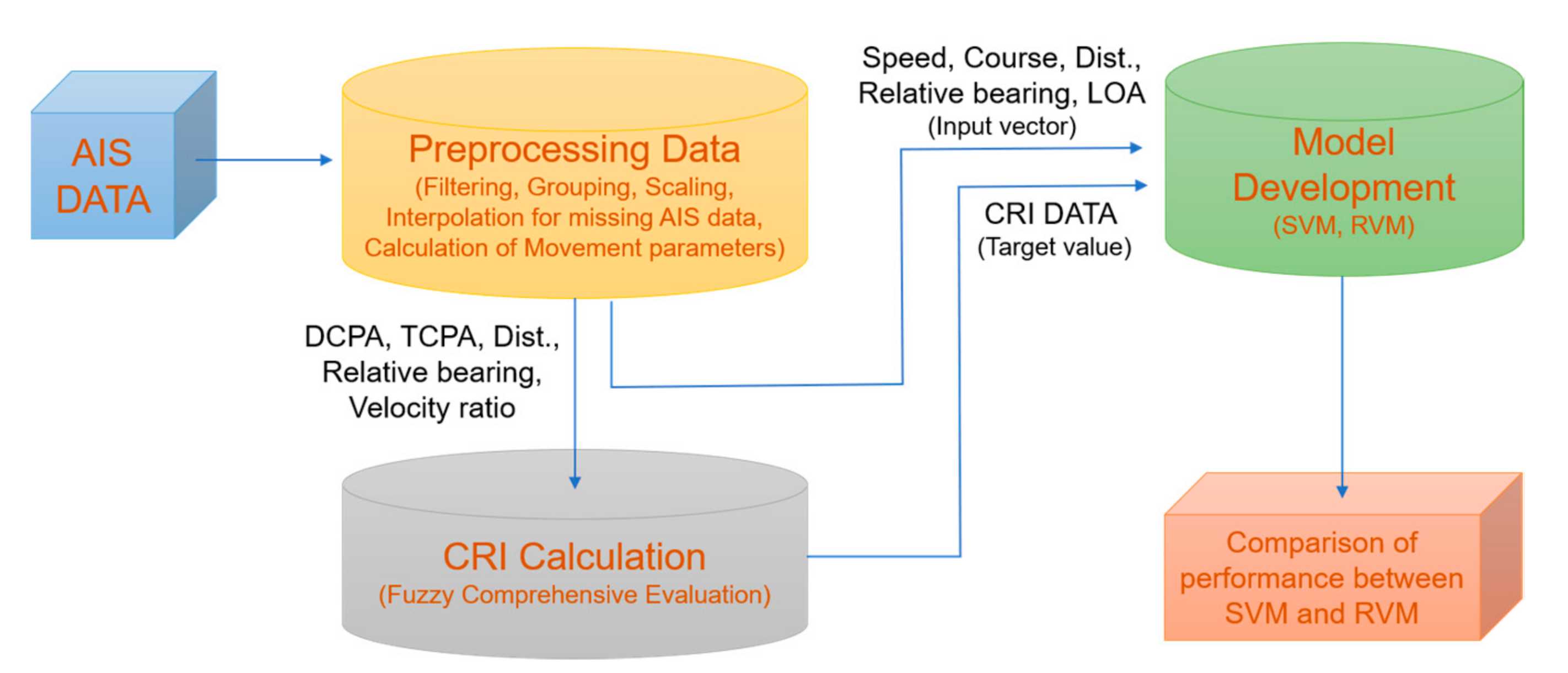
In order to estimate the CRI of encountering vessels, our approach followed the method illustrated in Figure 1. First, the AIS data were preprocessed to secure the variables used as input vectors and target values. The FCE method was used to obtain the CRIs used as the target values after that, and the SVM model and RVM model derived at the model development stage were compared and analyzed.

2.1. Preprocessing AIS Data

AIS data contain inaccurate information, and some information is missing. Thus, it is crucial to preprocess the AIS data to ensure it is accurate and efficient. We used methods for filtering, grouping, and scaling. According to the performance standards of shipborne AIS required by the International Maritime Organization (IMO), the static information should be updated every 6 min or on demand, and the dynamic information should be reported at a minimum interval of 2 s to 3 min depending on the speed of the vessel [19]. However, among the collected AIS data, the dynamic information of most vessels was not updated according to the performance standards. Therefore, it is necessary to interpolate the missing dynamic information in order to estimate the risk of collision between vessels at the same time with a repeat interval. In this study, using the MATLAB software, the observed position, speed, and course data of all target vessels were interpolated at 1 s intervals by applying the spline function for each interval.

Moreover, as shown in Figure 1 above, in order to calculate CRI and develop an estimated model, the values of various variables must be derived. In this study, DCPA, TCPA, distance (D), relative bearing (B), and velocity ratio (K) were selected as target factors among the many factors affecting CRI to calculate CRI by FCE method. In the Cartesian coordinate system, it is assumed that its origin is the position of the own vessel, (X, Y) denotes the coordinates corresponding to the relative position of the target vessel, $V_o$ denotes the true velocity of the own vessel, $V_t$ denotes the true velocity of the target vessel, $V_r$ denotes the relative velocity of the target vessel with respect to the own vessel, and $V_{rx}$, $V_{ry}$ denote the components of $V_r$. Based on this assumption, we can obtain the DCPA, TCPA, D, and K as follows [20,21]:

$$DCPA=\left|\frac{X{V}_{ry}-Y{V}_{rx}}{V_r}\right|$$

(1)

$$TCPA=-\frac{X{V}_{rx}+Y{V}_{ry}}{V_r^2}$$

(2)

$$D=\sqrt{X^2+Y^2}$$

(3)

$$K=V_t / V_o$$

(4)

2.2. CRI Calculation

According to FCE method, CRI can be obtained by the dot product of weight vector and membership vector as follows [3,10]:

$$CRI=W·U=W_{DCPA}·U_{DCPA}+W_{TCPA}·U_{TCPA}+W_D·U_D+W_B·U_B+W_K·U_K$$

(5)

where W denotes the weight vector of target factors. It was determined by using the analytic hierarchy process (AHP), which is a measurement theory for deriving priority scales through pairwise comparisons based on the judgments of experts [22]. According to this process, we surveyed the experts of navigation and constructed the set of pairwise comparison matrices to calculate the weight values of each target factor. As a result, the following weight vector was obtained [21]:

$$W=\left[W_{\mathrm{DCPA}}, W_{\mathrm{TCPA}}, W_{\mathrm{D}}, W_{\mathrm{B}}, W_{\mathrm{K}}\right]=\left[0.4457, 0.2258, 0.1408, 0.1321, 0.0556\right].$$

(6)

$U$ denotes the membership vector of target factors. The greater the membership value, the greater the collision risk of encountered vessels. The membership value of each target factor could be obtained through the following membership functions as applied in [3,12,17,21,23]:

DCPA is the most important factor that is considered as a spatial indicator of collision risk, and the smaller the value of DCPA, the greater the collision risk. The membership function of DCPA is as follows:

$$U_{DCPA}=\left\{\begin{array}{c}1, \left|DCPA\right|<d_1\\ {\left(\frac{d_2-\left|DCPA\right|}{d_2-d_1}\right)}^2 d_1\le \left|DCPA\right|\le \\ 0, \left|DCPA\right|>d_2\end{array}\right.d_2$$

(7)

where $d_1$ denotes the minimum safety distance between encountered vessels and $d_2$ denotes the absolute safety distance, which is equal to twice the value of $d_1$. The value of $d_1$ can be obtained as follows:

$$d_1=\left\{\begin{array}{c}1.1, 355°<B\le 67.5°\\ 1, 67.5°<B\le 112.5°\\ 0.6, 112.5°<B\le 247.5°\\ 0.9, 247.5°<B\le 355°\end{array}\right.$$

(8)

TCPA represents a temporal indicator of collision risk, and the smaller the value of TCPA, the greater the collision risk of encountered vessels. The membership function of TCPA is as follows:

$$U_{TCPA}=\left\{\begin{array}{c} 1 0\le \left|TCPA\right|\le t_1\\ {\left(\frac{t_2-\left|TCPA\right|}{t_2-t_1}\right)}^2 t_1\le \left|TCPA\right|\le t_2\\ 0 \left|TCPA\right|>t_2\end{array}\right.$$

(9)

where $t_1$ denotes the time remaining until collision and $t_2$ denotes the collision avoidance time. $t_1$ and $t_2$ can be obtained as follows:

$$t_1=\left\{\begin{array}{c}\frac{\sqrt{d_1^2-DCP{A}^2}}{V_R} DCPA\le d_1\\ 0 DCPA>d_1\end{array}\right.$$

(10)

$$t_2=\left\{\begin{array}{c}\frac{\sqrt{d_2^2-DCP{A}^2}}{V_R} DCPA\le d_2\\ 0 DCPA>d_2\end{array}\right.$$

(11)

The membership function of D is as follows:

$$U_D=\left\{\begin{array}{c} 1 0<D<D_1\\ {\left(\frac{D_2-D}{D_2-D_1}\right)}^2{D}_1\le D\le D_2\\ 0 D>D_2 \end{array}\right.$$

(12)

where $D_1$ denotes critical safety distance and equals 12 times the length of the own vessel ($L_o$); i.e., $D_1=12L_o$. $D_2$ denotes the distance at which the final action of collision avoidance can be taken. $D_2$ can be obtained as follows:

$$D_2=1.7\cos \left(B-19°\right)+\sqrt{4.4+2.89{\cos }^2\left(B-19°\right)}$$

(13)

The membership function of B is as follows:

$$U_B=\frac{1}{2}\left[ \cos \left(B-19°\right)+\sqrt{\frac{440}{289}+{\cos }^2\left(B-19°\right)}\right]-\frac{5}{17}$$

(14)

The membership function of K is as follows:

$$U_K=\frac{1}{1+\frac{2}{K\sqrt{K^2+1+2K\sin C}}}$$

(15)

2.3. Model Development

We modeled the dataset, applying SVM regression and RVM regression separately. A dataset of input vectors ${\left\{{\mathrm{x}}_n\right\}}_{n=1}^N$ with corresponding target values ${\left\{t_n\right\}}_{n=1}^N$ is required in the modeling process. The variables used as input vectors are the distance (D), relative bearing (B), the own vessel ($V_o$), velocity of the target vessel ($V_t$), course of the own vessel ($C_o$), course of the target vessel ($C_t$), length of the own vessel ($L_o$), and length of the target vessel ($L_t$). Unlike in [3], the length of the vessel was included in the input vectors for improving the estimation, considering that the risk of collision depends on the length of the target vessel in an encountering situation under the same condition. The target values refer to the CRI calculated by FCE method. All procedures of the model development were carried out using MATLAB software.

2.3.1. SVM Regression

The SVM is a supervised learning tool for classification and regression analysis using the optimal separating hyperplane that is built through some fixed nonlinear transformation that maps the input vectors into the high-dimensional feature space. It was first introduced by Vladimir Vapnik, Bernhard Boser, and Isabelle Guyon in 1992 [24] and was generalized by Vladimir Vapnik and Corinna Cortes in 1995 [25]. As indicated in [26], the details of SVM regression are as follows:

Suppose we are given a dataset of observed pairs comprising input vectors with corresponding target values ${\left\{{\mathrm{x}}_n, t_n\right\}}_{n=1}^N$ in order to obtain a solution in the form

$$y\left(\mathrm{x}\right)={\mathrm{w}}^{\mathrm{T}}\varphi \left(\mathrm{x}\right)+b,$$

(16)

where $\mathrm{w}$ denotes the weight vectors, $\varphi \left(\mathrm{x}\right)$ denotes a fixed function that maps the input vectors into the high-dimensional feature space, and $b$ denotes the bias parameter. We have to define $\mathrm{w}$ and $b$.

To obtain sparse solutions, the $ϵ$-insensitive loss function was used as follows:

$${\left|y\left(\mathrm{x}\right)-t\right|}_{ϵ}=\left\{\begin{array}{c}0 if \left|y\left(x\right)-t\right|\le ϵ\\ \left|y\left(x\right)-t\right|-ϵ \mathrm{otherwise}\end{array}\right.$$

(17)

The loss is equal to 0 if the discrepancy between the predicted and the target values is less than $ϵ$. Therefore, we have to minimize the following regularized objective function:

$$C{\displaystyle \sum }_{n=1}^N{\left|y\left({\mathrm{x}}_n\right)-t_n\right|}_{ϵ}+\frac{1}{2}\parallel \mathrm{w}{\parallel }^2$$

(18)

where the last term penalizes the model for using more weight vectors and makes it as flat as possible. The parameter $C$ in the first term determines the relative importance of the loss term compared with the penalty term and helps to avoid overfitting. This optimization problem can be transformed into a problem that minimizes the following function by introducing slack variables ${\mathsf{\xi }}_n$ and ${\mathsf{\xi }}_n^{*}$ for each data point:

$$C{\displaystyle \sum }_{n=1}^N\left({\mathsf{\xi }}_n+{\mathsf{\xi }}_n^{*}\right)+\frac{1}{2}\parallel \mathrm{w}{\parallel }^2$$

(19)

subject to the constraints

$$t_n-y\left({\mathrm{x}}_n\right)\le ϵ+{\mathsf{\xi }}_n^{*} {\mathsf{\xi }}_n^{*}\ge 0$$

(20)

$$y\left({\mathrm{x}}_n\right)-t_n\le ϵ+{\mathsf{\xi }}_n {\mathsf{\xi }}_n\ge 0$$

(21)

To solve this problem, Lagrange multipliers ${\alpha }_n\ge 0$, ${\alpha }_n^{*}\ge 0$, ${\beta }_n\ge 0$, and ${\beta }_n^{*}\ge 0$ are introduced for each data point, and the Lagrangian is constructed as follows:

$$L=\frac{1}{2}\parallel \mathrm{w}{\parallel }^2+C{\displaystyle \sum }_{n=1}^{\mathrm{N}}\left({\mathsf{\xi }}_n+{\mathsf{\xi }}_n^{*}\right)-{\displaystyle \sum }_{n=1}^N{\alpha }_{\mathrm{n}}\left(t_n-y\left({\mathrm{x}}_n\right)+ϵ+{\mathsf{\xi }}_n\right)$$

(22)

$$-{\displaystyle \sum }_{n=1}^N{\alpha }_n^{*}\left(y\left({\mathrm{x}}_n\right)-t_n+ϵ+{\mathsf{\xi }}_n^{*}\right)-{\displaystyle \sum }_{n=1}^N\left({\beta }_n{\mathsf{\xi }}_n+{\beta }_n^{*}{\mathsf{\xi }}_n^{*}\right)$$

This Lagrangian whose is minimum over $\mathrm{w}$, ${\mathsf{\xi }}_n$, ${\mathsf{\xi }}_n^{*}$ leads to the following equations:

$$\mathrm{w}={\displaystyle \sum }_{n=1}^N\left({\alpha }_n^{*}-{\alpha }_n\right)\varphi \left({\mathrm{x}}_n\right)$$

(23)

$${\displaystyle \sum }_{n=1}^N\left({\alpha }_n-{\alpha }_n^{*}\right)=0$$

(24)

$${\alpha }_n^{*}+{\beta }_n^{*}=C {\alpha }_n+{\beta }_n=C$$

(25)

Substituting (23) into (16), we can obtain the desired function as follows:

$$y\left(\mathrm{x}\right)={\displaystyle \sum }_{n=1}^N\left({\alpha }_n^{*}-{\alpha }_n\right)K(\mathrm{x},{\mathrm{x}}_n)+b$$

(26)

where $K\left(\mathrm{x},{\mathrm{x}}_n\right)$ is the kernel function that generates the inner products in a high-dimensional feature space.

2.3.2. RVM Regression

The RVM is also a supervised learning tool for classification and regression analysis based on the Bayesian framework and provides posterior probabilistic outputs. It was first introduced by Tipping in 2000 [16]. As indicated in [15,16], the details of RVM regression are as follows:

Suppose we are given a dataset of observed pairs comprising input vectors with corresponding target values ${\left\{{\mathrm{x}}_n, t_n\right\}}_{n=1}^N$ and we assume $p(t|\mathrm{x})$ is Gaussian distribution $N(t|y\left(\mathrm{x}\right),{\mathsf{\sigma }}^2)$, where the mean $y\left(\mathrm{x}\right)$ is defined as

$$y\left(\mathrm{x}\right)={\displaystyle \sum }_{n=1}^N{w}_{n}K(\mathrm{x},{\mathrm{x}}_n)+w_0$$

(27)

This function has the same form as the function (16) for the SVM. The likelihood of the dataset can be written as

$$p\left(\mathrm{t}|\mathrm{w},{\sigma }^2\right)={\left(2\mathsf{\pi }{\sigma }^2\right)}^{-\frac{N}{2}}\exp \left\{-\frac{1}{2{\sigma }^2}\mathrm{t}-{\mathsf{\Phi }\mathrm{w}}^2\right\}$$

(28)

where $\mathrm{t}={\left(t_1. . .t_{\mathrm{N}}\right)}^{\mathrm{T}}, \mathrm{w}={\left(w_0. . .w_{\mathrm{N}}\right)}^{\mathrm{T}}$, and $\mathsf{\Phi }$ is the $N\times \left(N+1\right)$ ‘design’ matrix with $\mathsf{\Phi }={\left[\varphi \left({\mathrm{x}}_1\right)\dots \varphi \left({\mathrm{x}}_N\right)\right]}^{\mathrm{T}}$, wherein $\varphi ({\mathrm{x}}_n)={\left[1, K\left({\mathrm{x}}_n,{\mathrm{x}}_1\right), K\left({\mathrm{x}}_n,{\mathrm{x}}_2\right)\dots K\left({\mathrm{x}}_n,{\mathrm{x}}_N\right)\right]}^{\mathrm{T}}.$ The notation of the implicit conditioning upon the set of input vectors $\left\{x_n\right\}$ is omitted in (28) and subsequent expressions. Since the maximum-likelihood estimation of $\mathrm{w}$ and ${\sigma }^2$ from (28) lead to a data overfitting problem, a zero-mean Gaussian prior distribution over $\mathrm{w}$ is defined as

$$p\left(\mathrm{w}|\mathsf{\alpha }\right)={\displaystyle \prod }_{n=0}^{N}N\left(w_n|0,{\alpha }_n{}^{-1}\right)$$

(29)

with $\alpha$ as a vector of N + 1 hyperparameters. According to Bayes’ rule, the posterior distribution over $\mathrm{w}$ can be obtained as follows:

$$\mathrm{p}\left(\mathrm{w}|\mathrm{t},\mathsf{\alpha },{\sigma }^2\right)={\left(2\mathsf{\pi }\right)}^{-\frac{\left(N+1\right)}{2}}{\left|\mathsf{\Sigma }\right|}^{-\frac{1}{2}}\exp \left\{-\frac{1}{2}{\left(\mathrm{w}-\mathsf{\mu }\right)}^{\mathrm{T}}{\mathsf{\Sigma }}^{-1}\left(\mathrm{w}-\mathsf{\mu }\right)\right\}$$

(30)

where the posterior covariance and mean, respectively, are as follows:

$$\mathsf{\Sigma }={\left({\sigma }^{-2}{\mathsf{\Phi }}^{\mathrm{T}}\mathsf{\Phi }+\mathrm{A}\right)}^{-1}$$

(31)

$$\mathsf{\mu }={\sigma }^{-2}{\mathsf{\Sigma }\mathsf{\Phi }}^{\mathrm{T}}\mathrm{t}$$

(32)

with $\mathrm{A}=diag\left({\mathsf{\alpha }}_0,{ \mathsf{\alpha }}_1. . .{\mathsf{\alpha }}_{\mathrm{N}}\right)$.

The marginal likelihood is obtained by integrating out $\mathrm{w}$ for the hyperparameters

$$p\left(\mathrm{t}|\mathsf{\alpha },{\mathsf{\sigma }}^2\right)={\left(2\mathsf{\pi }\right)}^{-\frac{N}{2}}{\left|{\sigma }^2\mathrm{I}+{\mathsf{\Phi }\mathrm{A}}^{-1}{\mathsf{\Phi }}^{\mathrm{T}}\right|}^{-\frac{1}{2}}\exp \left\{-\frac{1}{2}{\mathrm{t}}^{\mathrm{T}}{\left({\sigma }^2\mathrm{I}+{\mathsf{\Phi }\mathrm{A}}^{-1}{\mathsf{\Phi }}^{\mathrm{T}}\right)}^{-1}\mathrm{t}\right\}$$

(33)

Since values of $\alpha$ and ${\sigma }^2$ that maximize (33) cannot be obtained in closed form, the alternative formulae are considered for their iterative re-estimation.

For $\alpha$, differentiation of (33), equating to zero, and rearranging give:

$${\alpha }_n^{\mathrm{new}}=\frac{{\gamma }_n}{{\mu }_n^2}$$

(34)

where ${\mu }_n$ is the n-th posterior mean weight from (32) and the quantities ${\gamma }_n\in \left[0, 1\right]$ are defined as

$${\gamma }_n\equiv 1-{\alpha }_n{\mathsf{\Sigma }}_{nn}$$

(35)

with ${\mathsf{\Sigma }}_{nn}$ as the n-th diagonal element of the posterior weight covariance from (31) computed with the current $\alpha$ and ${\sigma }^2$ values.

For the noise variance ${\sigma }^2$, differentiation leads to the re-estimate

$${({\sigma }^2)}^{\mathrm{new}}=\frac{\parallel \mathrm{t}-\mathsf{\Phi }\mathsf{\mu }{\parallel }^2}{N-{{\displaystyle \sum }}_n{\gamma }_n}$$

(36)

2.4. Parameter Optimization

In order to obtain a model that estimates the risk of vessel collision properly, a process of optimizing the parameters that affect the estimation performance is required. In this study, a method of partitioning the dataset into a training set and a validation set was applied. We inputted the validation set to the model trained with the training set to estimate the CRI ($\widehat{CRI}$), and we selected the optimal parameters that minimize the differences between the $\widehat{CRI}$ and the target value (CRI). The model that shows the lower estimation error for the new dataset possesses a successful generalization performance, so the data overfitting problem can be solved. The root mean square error (RMSE) was calculated to measure the estimation error. The Gaussian kernel function is applied for both SVM and RVM. This kernel function is as follows.:

$$\mathrm{K}\left(\mathrm{x},x_n\right)=\exp \left\{-\frac{x-x_n{}^2}{2{\sigma }^2}\right\}$$

(37)

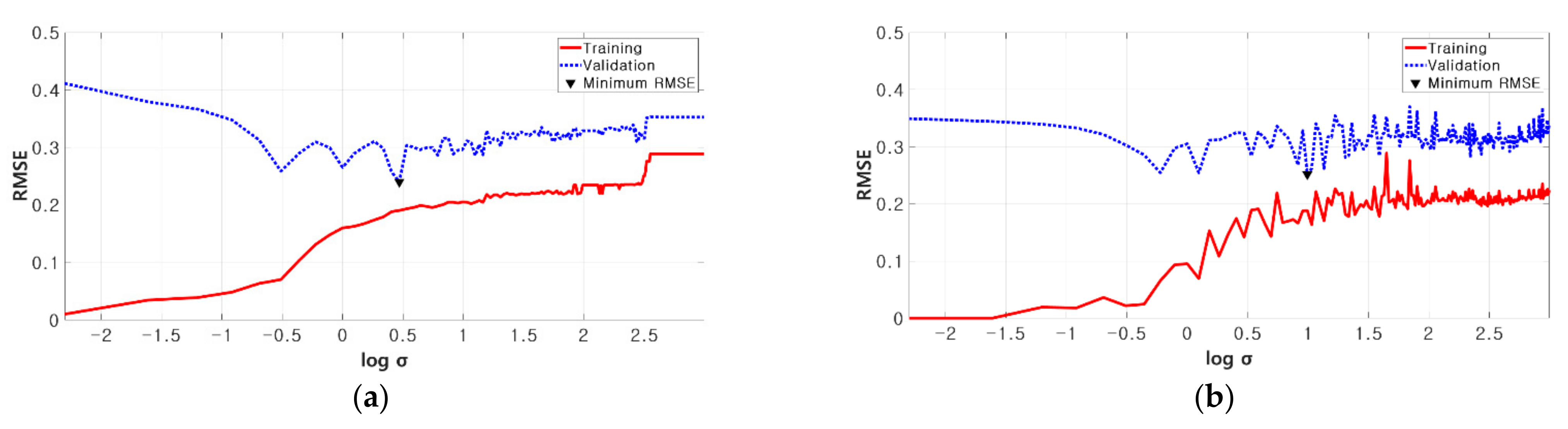
where the $\sigma$ denotes the kernel width to be optimized for both RVM and SVM. In order to optimize the parameter $\sigma$, the range of candidate values was specified as [0.1, 20]. By applying all the values within the range, the value that minimizes the RMSE for the verification set was determined as the best $\sigma$. In the case of SVM, additionally, parameters C and $ϵ$ were optimized with 4-fold cross-validation. Figure 2 shows the optimization process both of RVM (left) and SVM (right) as the change of RMSE with respect to the log$\sigma$.

3. Simulations and Results

3.1. Data Collection

Table 1. Vessel entry/departure and marine accidents by major ports of Korea (2014–2018).

Content	Year	Busan	Ulsan	Gwangyang	Incheon	Pyeongtaek
No. of vessel entry/ departure	2014	95,378	51,565	46,746	35,363	18,591
	2015	98,087	51,525	48,229	37,560	19,383
	2016	100,197	50,495	52,263	37,407	19,924
	2017	99,687	48,182	51,269	36,215	19,442
	2018	94,816	46,664	48,225	31,351	18,829
	Total	488,165	248,431	246,732	177,896	96,169
No. of marine accidents	2014	45	25	6	14	1
	2015	66	58	11	22	5
	2016	85	47	13	37	11
	2017	52	52	27	22	10
	2018	19	30	16	43	20
	Total	267	212	73	138	47

shows the volume of vessel traffic and the number of marine accidents by major ports of Korea in the last 5 years [2,27]. According to this table, the port with the largest number of vessel entries and departures and the largest number of marine accidents is Busan port. Therefore, in this study, we selected all vessels that were equipped with AIS and navigated in the predetermined area of 1453 km² in the vicinity of the entrance to Busan port as objects of research for the use of actual AIS data.

In order to be used as input data in the model development process, AIS data of vessels detected in the above-mentioned area from 1 to 3 April 2014 were selected. A total of 543 vessels were detected, and the static information such as vessel’s name, maritime mobile service identity (MMSI), and vessel’s length and the dynamic information such as vessel’s position (latitude and longitude), speed, and course were selected as variables for systematic analysis. After selecting the variables, a spreadsheet composed of the variables was created, and then all data for each variable were entered. A total of 2350 datasets were prepared through the collection and above-mentioned preprocessing of actual AIS data in the target sea area. The total of 2350 preparatory datasets were partitioned into 2000 training sets and 350 validation sets.

3.2. Results of Model Development

Table 2. Comparison of SVM and RVM models.

Method	$\mathbf{Best} \mathit{\sigma }$	Elapsed Time (min)	SVs/RVs	MAE	RMSE
SVM	2.7	8.73	634	0.2349	0.2518
RVM	1.6	0.14	129	0.2145	0.2401

shows the results of regression analysis for the estimation of CRI using SVM and RVM after the previous process of the parameter optimization. As a result of comparison, the values of RMSE and MAE show that the RVM model estimates more accurately than the SVM model. Furthermore, it was also shown that the number of vectors required in the RVM model (relevance vectors (RVs)) is much smaller than that in the SVM model (support vectors (SVs)), so the RVM model reduced the use of unnecessary basis functions. We can also see that the elapsed time of the RVM model for learning of data is significantly shorter than that of the SVM model. These results indicate that the RVM has higher accuracy and a faster, more efficient learning process compared to the SVM.

3.3. Model Validation

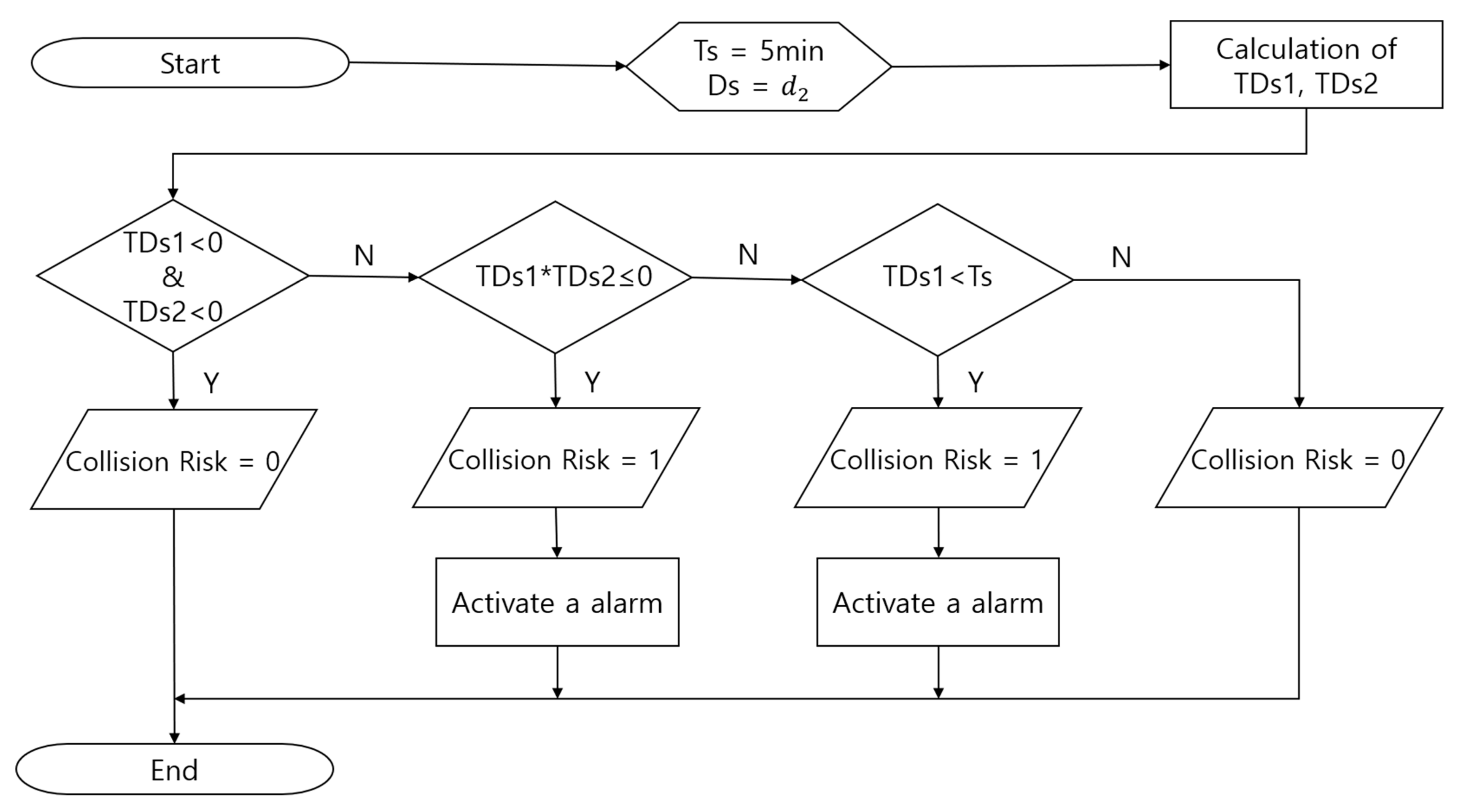
In order to validate the models developed by SVM and RVM, as indicated in [20], the algorithm for the detection of collision risk was applied [21]. The algorithm detects collision risk stably by introducing the time to safe distance ($\mathrm{TDs}$), which is the time required to reach the safety distance (Ds) between encountering vessels. If the $\mathrm{TDs}$ exists, it has two values represented by the following equations:

$$\mathrm{TDs}1=\mathrm{TCPA}-t_2$$

(38)

$$\mathrm{TDs}2=\mathrm{TCPA}+t_2$$

(39)

where $t_2$ denotes the time required to reach DCPA from Ds for the distance between encountering vessels. Figure 3 is a flowchart for the detection of collision risk. The value of Ds was applied by the value of $d_2$, which was used to calculate the CRI, and the threshold value of $TDs$ (Ts) was set to 5 min to run the algorithm. The outputs of the algorithm were programmed using a binary number to display a value of 1 if the risk of collision exists and a value of 0 if not. The dataset used as a test dataset in the previous modeling and the AIS data of head-on situations in which a real risk of collision exists were used as the verification data.

3.4. Results of Simulations

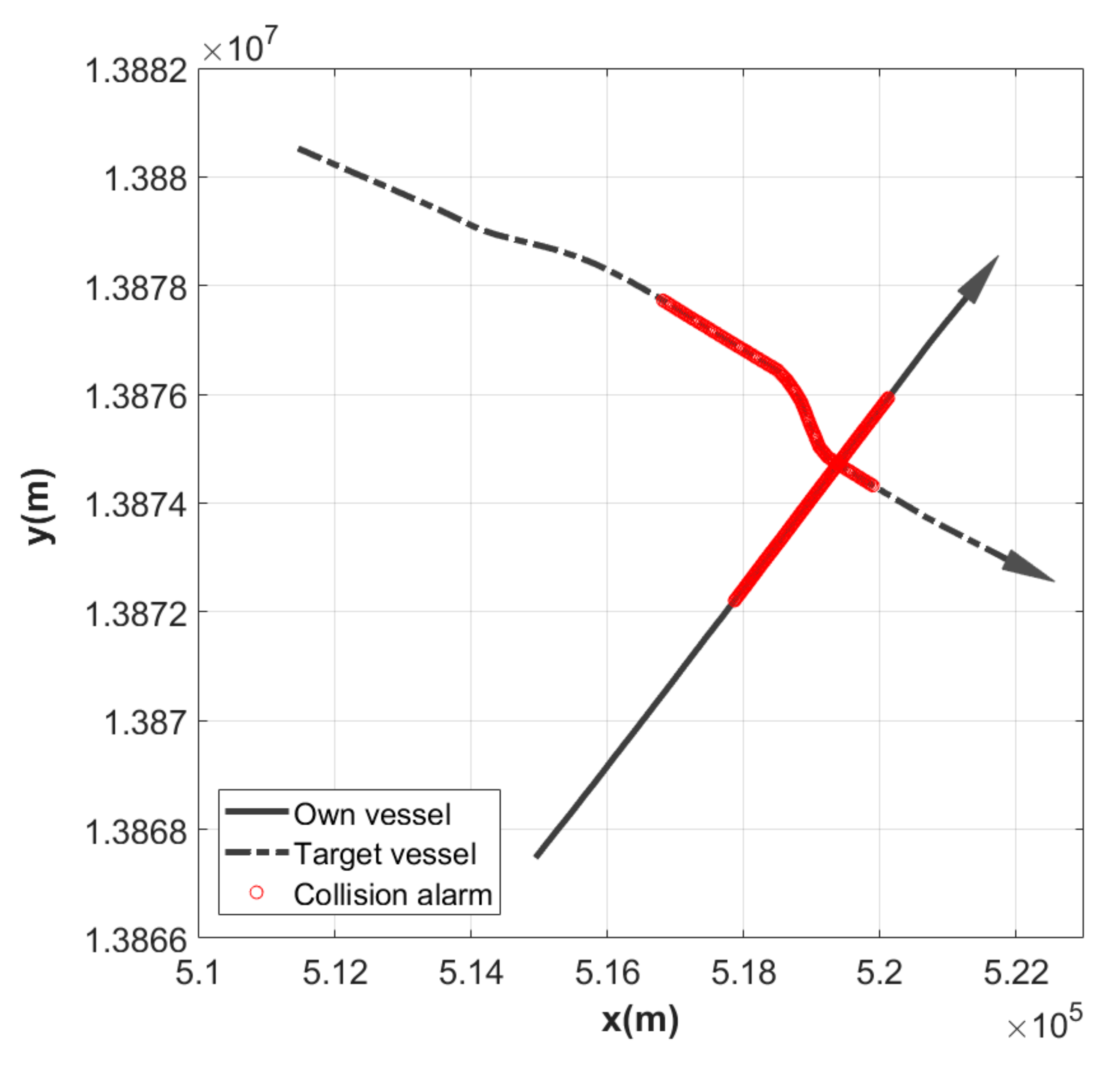
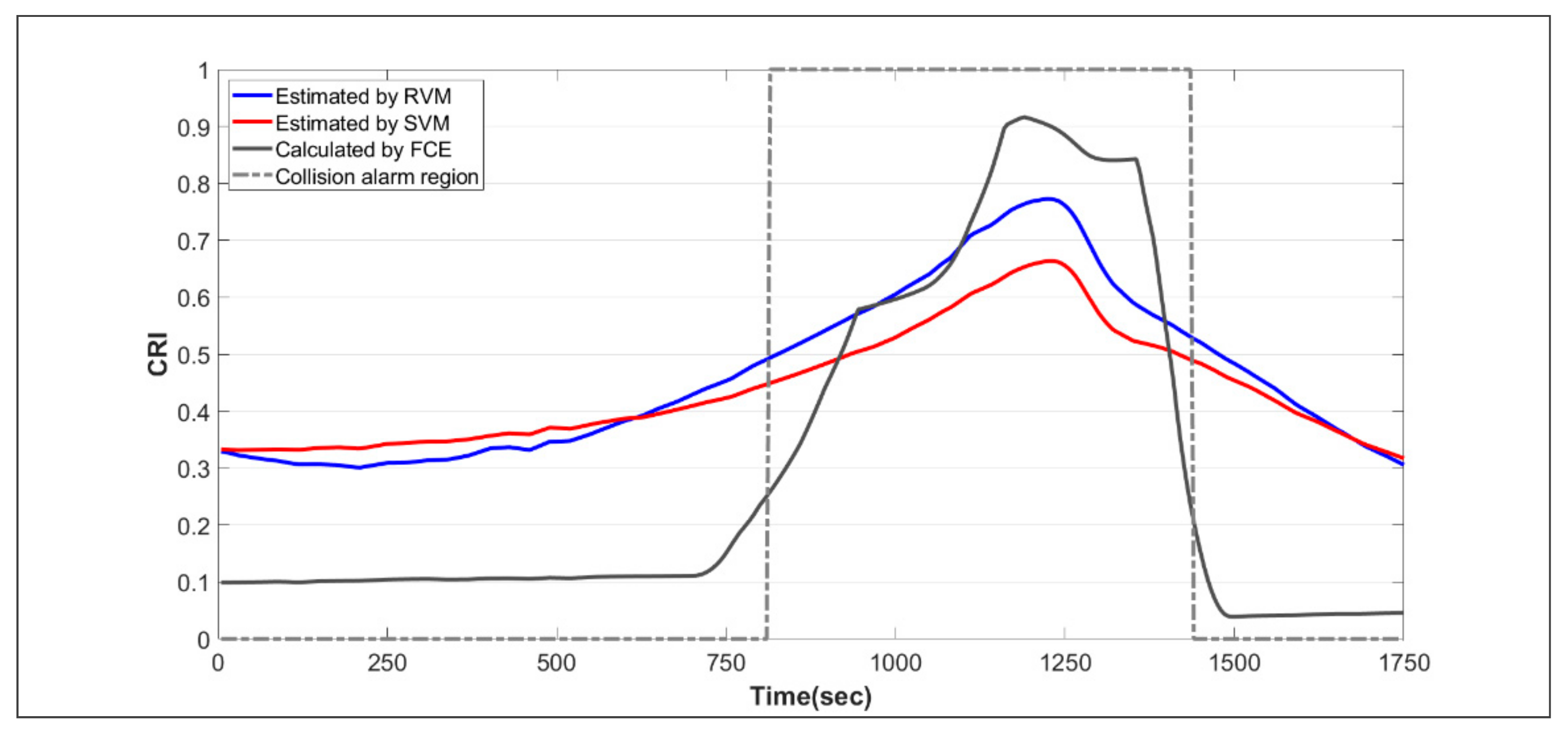
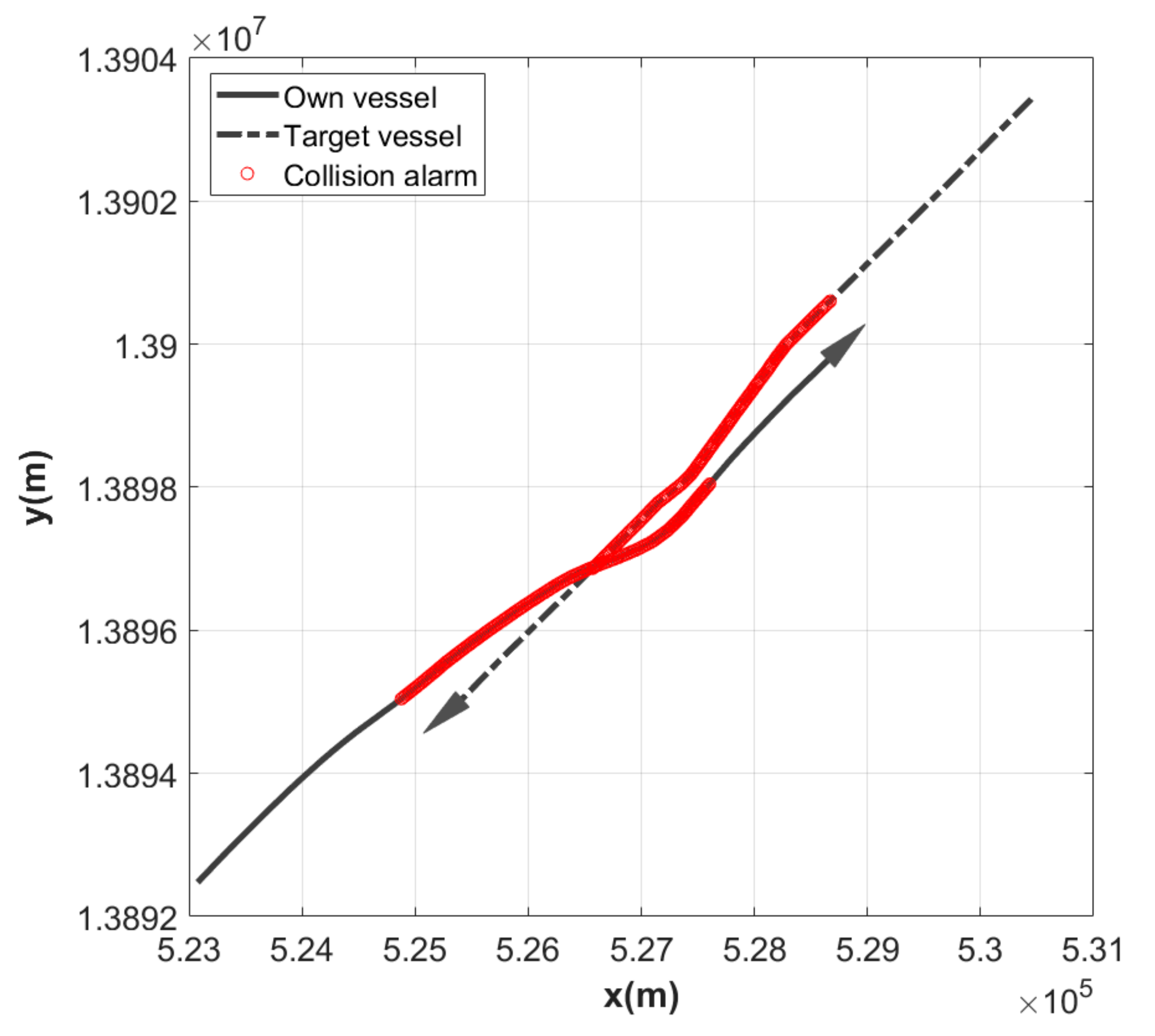
The actual AIS data of the crossing situation between the two vessels were used for the validation of the developed model. Figure 4 shows the trajectory of the vessels, displaying the section where the alarm occurred for each vessel based on the algorithm for the detection of collision risk. According to Figure 4, we can see that the target vessel altered her course to starboard to avoid collision with the own vessel. Figure 5 represents the results of estimating CRI for this situation using the developed SVM and RVM models. The maximum CRI values for each model are shown in the region of the collision alarm. Although each time point corresponding to the maximum value of CRI is similar for all models, the highest value of CRI is 0.92 for the FCE model, and the lowest value of CRI is 0.66 for the SVM model. Moreover, among the minimum CRI values at which an alarm occurred for each model in the region of collision alarm, the highest value is 0.5 for the RVM model and the lowest value is 0.2 for the FCE model.

The actual AIS data of the head-on situation between the two vessels were used for additional verification. Figure 6 shows the trajectory of the vessels, displaying the section where the alarm occurred for each vessel based on the algorithm for the detection of collision risk. According to Figure 6, we can see that the own vessel altered her course to starboard to avoid collision with the target vessel. Figure 7 represents the results of estimating CRI for this situation using the developed SVM and RVM models. The maximum CRI values for each model are shown in the region of the collision alarm. Although each time point corresponding to the maximum value of CRI is similar for all models, the highest value of CRI is 0.92 for the FCE model, and the lowest value of CRI is 0.71 for the SVM model. Moreover, among the minimum CRI values at which an alarm occurred for each model in the region of collision alarm, the highest value is 0.62 for the RVM model and the lowest value is 0.19 for the FCE model. Similar to the crossing situation, in the region of collision alarm, it was found that the CRI value of the FCE model shows a steep curve, while each CRI value of the RVM and SVM models shows a gentle curve.

4. Discussion

In this study, we developed the models of SVM and RVM for estimating CRI using actual AIS data, which were collected from the coastal sea area of the entrance to Busan port in Korea. We focused on comparing RVM and SVM under the same conditions as much as possible in the process of optimizing the parameters. As a result of the comparison between SVM and RVM, it was shown that the accuracy of each CRI estimated by inputting a new dataset into the developed models was higher for the RVM model than the SVM model. It was confirmed that the RVM model avoids the data overfitting problem and represents successful generalization performance. In addition, we confirmed that the computational complexity of RVM was lower than SVM since the number of basis functions required for the SVM model was shown to be about 5 times that of the RVM model, and the time required to create the RVM model was much shorter than that to create the SVM model, so the efficiency of learning data was improved by RVM. As verification results of estimation performance through applying the two cases, the FCE model has a collision alarm in the CRI range of [0.19, 0.92], so the model represented too broad a range of collision risk because the range of the CRI was defined as [0,1]. However, the time point at which the highest collision risk appeared was similar to other models. In contrast, the RVM model has a collision alarm in the CRI range of [0.5, 0.89], and the SVM model has a collision alarm in the CRI range of [0.45, 0.71]. Considering that the actions for collision avoidance were taken in both encounter cases used for the verification, we can know that the collision of risk was very high in the two cases. So, it is judged that the estimation performance of the RVM model is better than that of the SVM model, since the overall CRI estimated by the RVM is higher than that of the SVM. In the case of the RVM model developed through this research, it must be determined that there is a risk of collision if the CRI reaches the value of 0.5 on the actual voyage. In order to properly verify the accuracy of this result, a comparison with the CRI estimated by the actual navigator at the time is required. In addition, the CRI estimation should be improved so that it can be applied even in the case of encounters with several target vessels at the same time. If more experts’ evaluations are additionally reflected in the FCE method, the proposed method can be further improved. Accurate and rapid collision risk estimation can have a good effect on the development of an excellent collision avoidance algorithm.

5. Conclusions

As described in Section 1, in order to prevent collision accidents, it is necessary to assist individual navigators in the decision-making on the existence of collision risk. In this study, we utilized actual AIS data to observe the CRI by the FCE method. Then, based on the RVM and SVM, we developed the models for estimating the CRI between the encountering vessels under the same conditions. As a result of comparing the two developed models, the RVM model showed better performance by solving the shortcomings of the SVM model. In addition, the comparison results of the developed model were validated through case studies such as crossing situations and head-on situations. In particular, the CRI value calculated using FCE has too broad a range of the collision alarm, making it difficult to specify the quantitative risk range. However, in the case of the RVM model, since the alarm of collision risk was generated from the CRI value of 0.5, this value can be defined as the threshold value at which the action of collision avoidance is required.

We confirmed the possibility for accurate and intuitional assistance in determining whether the risk of collision exists through the real-time estimation of CRI by machine learning on the actual voyage. In order to establish a collision risk estimation system applicable to actual navigation, further simulations considering human factors and navigator’s experience and skill level are required in the future. In this study, we focused on improving conventional machine learning, and we will apply advanced machine learning in the future. Comparing the results of the proposed method with the state-of-the-art approaches will help to improve the estimation performance for CRI. It is expected to be of great assistance in the development of a practical system that can automatically take collision avoidance actions based on COLREGS and optimize the vessel’s route in real time.

References

- IMO (International Maritime Organization). COLREGS—International Regulations for Preventing Collisions at Sea. In Convention on the International Regulations for Preventing Collisions at Sea; IMO (International Maritime Organization): London, UK, 1972; pp. 1–74. [Google Scholar]
- KMST (Korean Maritime Safety Tribunal). 2020 Annual Report of Marine Accident Statistics. Available online: https://www.kmst.go.kr (accessed on 10 March 2020).
- Gang, L.; Wang, Y.; Sun, Y.; Zhou, L.; Zhang, M. Estimation of vessel collision risk index based on support vector machine. Adv. Mech. Eng. 2016, 8, 1–10. [Google Scholar] [CrossRef] [Green Version]
- Ahn, J.H.; Rhee, K.P.; You, Y.J. A study on the collision avoidance of a ship using neural networks and fuzzy logic. Appl. Ocean Res. 2012, 37, 162–173. [Google Scholar] [CrossRef]
- Li, C.; Li, W.; Ning, J. Calculation of Ship Collision Risk Index Based on Adaptive Fuzzy Neural Network; Atlantis Press: Paris, France, 2018. [Google Scholar]
- Kearon, J. Computer program for collision avoidance and track keeping. In Proceedings of the International Conference on Mathematics Aspects of Marine Traffic; Academic Press: London, UK, 1977; pp. 229–242. [Google Scholar]
- Imazu, H.; Koyama, T. The Determination of Collision Avoidance Action. J. Jpn. Inst. Navig. 1984, 70, 31–37. [Google Scholar] [CrossRef] [Green Version]
- Zec, D. An Algorithm for a Real-Time Detection of Encounter Situations. J. Navig. 1996, 49, 121–126. [Google Scholar] [CrossRef] [Green Version]
- Chin, H.C.; Debnath, A.K. Modeling perceived collision risk in port water navigation. Saf. Sci. 2009, 47, 1410–1416. [Google Scholar] [CrossRef] [Green Version]
- Xu, Q.; Meng, X.; Wang, N. Intelligent evaluation system of ship management. Mar. Navig. Saf. Sea Transp. 2009, 4, 787–790. [Google Scholar] [CrossRef]
- Zhao, Y.; Li, W.; Shi, P. A real-time collision avoidance learning system for Unmanned Surface Vessels. Neurocomputing 2016, 182, 255–266. [Google Scholar] [CrossRef]
- Li, B.; Pang, F.W. An approach of vessel collision risk assessment based on the D-S evidence theory. Ocean Eng. 2013, 74, 16–21. [Google Scholar] [CrossRef]
- Zadeh, L.A. Simple View of the Dempster-Shafer Theory of Evidence and Its Implication for the Rule of Combination. AI Mag. 1986, 7, 85–90. [Google Scholar]
- Voorbraak, F. On the justification of Dempster’s rule of combination. Artif. Intell. 1991, 48, 171–197. [Google Scholar] [CrossRef] [Green Version]
- Tipping, M.E. The relevance vector machine. In Proceedings of the Advances in Neural Information Processing Systems; Solla, S.A., Leen, T.K., Müller, K.-R., Eds.; MIT Press: Cambridge, MA, USA, 2000; Volume 12, pp. 653–658. [Google Scholar]
- Tipping, M.E. Sparse Bayesian Learning and the Relevance Vector Machine. J. Mach. Learn. Res. 2001, 1, 211–244. [Google Scholar] [CrossRef] [Green Version]
- Zhou, J.H.; Wu, C.J. The construction of the collision risk factor model. J. Ningbo Univ. 2004, 17, 61–65. [Google Scholar]
- Ren, Y.; Mou, J.; Yan, Q.; Zhang, F. Study on assessing dynamic risk of ship collision. In Proceedings of the ICTIS 2011: Multimodal Approach to Sustained Transportation System Development: Information, Technology, Implementation, Wuhan, China, 30 June–2 July 2011; pp. 2751–2757. [Google Scholar]
- IMO (International Maritime Organization). Adoption of New and Amended Performance Standards for Navigational Equipment; IMO (International Maritime Organization): London, UK, 1998; Volume 86, pp. 13–16. [Google Scholar]
- Lenart, A.S. Analysis of Collision Threat Parameters and Criteria. J. Navig. 2015, 68, 887–896. [Google Scholar] [CrossRef] [Green Version]
- Park, J.; Jeong, J. Assessment of Ship Collision Risk in Coastal Waters by Fuzzy Comprehensive Evaluation. J. Korean Inst. Intell. Syst. 2020, 30, 325–330. [Google Scholar] [CrossRef]
- Saaty, T.L. Decision making with the Analytic Hierarchy Process. Int. J. Serv. Sci. 2008, 1, 83–98. [Google Scholar] [CrossRef] [Green Version]
- Nguyen, M.; Zhang, S.; Wang, X. A novel method for risk assessment and simulation of collision avoidance for vessels based on AIS. Algorithms 2018, 11, 204. [Google Scholar] [CrossRef] [Green Version]
- Vapnik, V.N. The Nature of Statistical Learning Theory; Springer: New York, NY, USA, 1995. [Google Scholar]
- Vapnik, V. Estimation of Dependences Based on Empirical Data; Springer Science & Business Media: Berlin/Heidelberg, Germany, 2006; ISBN 0387342397. [Google Scholar]
- Vapnik, V.; Vapnik, V. Statistical Learning Theory; Wiley: New York, NY, USA, 1998; Volume 1. [Google Scholar]
- Ministry of Oceans and Fisheries Statistics of Vessels Arrival and Departure at Major Port of Korea. Available online: http://www.mof.go.kr (accessed on 8 January 2020).
Figure 1.
Proposed method for estimating the CRI with AIS data.
Figure 2.
Process of optimizing the parameter for RVM (a) and SVM (b).
Figure 3.
Flowchart for the detection of collision risk.
Figure 4.
Trajectories of encountering vessels in the case of crossing situation.
Figure 5.
Results of estimation in the case of crossing situation.
Figure 6.
Trajectories of encountering vessels in the case of head-on situation.
Figure 7.
Results of estimation in the case of head-on situation.