A Multifaceted Approach to Advance Oil Spill Modeling and Physical Oceanographic Research at the United States Bureau of Ocean Energy Management

Abstract

The Environmental Studies Program (ESP) at the United States Bureau of Ocean Energy Management (BOEM) is funded by the United States Congress to support BOEM’s mission, which is to use the best available science to responsibly manage the development of the Nation’s offshore energy and mineral resources. Since its inception in 1973, the ESP has funded over $1 billion of multidisciplinary research across four main regions of the United States Outer Continental Shelf: Gulf of Mexico, Atlantic, Alaska, and Pacific. Understanding the dynamics of oil spills and their potential effects on the environment has been one of the primary goals of BOEM’s funding efforts. To this end, BOEM’s ESP continues to support research that improves oil spill modeling by advancing our understanding and the application of meteorological and oceanographic processes to improve oil spill modeling. Following the Deepwater Horizon oil spill in 2010, BOEM has invested approximately $28 million on relevant projects resulting in 73 peer-reviewed journal articles and 42 technical reports. This study describes the findings of these projects, along with the lessons learned and research information needs identified. Additionally, this paper presents a path forward for BOEM’s oil spill modeling and physical oceanographic research.

1. Introduction

The tragic incident of the Deepwater Horizon (DWH) oil spill in the Gulf of Mexico (GOM) killed 11 crewmen and resulted in $71 billion in response costs, penalties and damages (according to the latest estimate as of 18 April 2020 [1]). The DWH incident also marked the beginning of an unprecedented level of oil spill research efforts. Shortly after the DWH disaster, BP announced a commitment of up to $500 million over 10 years to fund an independent research program, the Gulf of Mexico Research Initiative (GoMRI), designed to study the impact of the oil spill and its associated response to the environment and public health [2]. In 2013, the legal settlements with BP and Transocean led to the creation of the Gulf Research Program at the National Academy of Sciences (NAS). The 30-year program aims to improve the safety of oil and gas development and transportation and the potential impacts they pose to public health and the environment in the GOM and other Outer Continental Shelf (OCS) regions in the United States (U.S.) [3]. Before the DWH oil spill, the Bureau of Ocean Energy Management (BOEM) and its predecessor, the Minerals Management Service (MMS), was a major source of funding for oceanographic research in the GOM [4] and other OCS regions. The outcomes and expertise developed through BOEM’s Environmental Studies Program (ESP) provided critical information to the response efforts during and after the DWH event [5]. Now, as the GoMRI program comes to a close, BOEM continues to support oil spill research efforts on the OCS. In this paper, we review relevant oil spill modeling and physical oceanographic studies funded by BOEM’s ESP over the last decade, while identifying potential information needs and establishing a strategy for future research efforts in these areas.

The Outer Continental Shelf Lands Act (OCSLA; 43 U.S.C. 1331 et seq.) mandates that the Secretary of the U.S. Department of the Interior (DOI) conduct environmental studies and provide information to assess and monitor the potential impacts to human, marine, and coastal environments from offshore energy development. The U.S. OCS, as defined by OCSLA, consists of all submerged lands in U.S. waters that are 3 nautical miles (nm) seaward of state waters, except Texas and the Gulf Coast of Florida, which are extended 3 marine leagues (9 nm) offshore from the baseline.

Established by the U.S. Congress in 1973, the ESP at BOEM, an agency under DOI, supports research efforts intended to inform decision makers on the development of oil and gas, renewable energy, and marine mineral resources on the OCS. The ESP has provided over $1 billion for research since its inception. Much of the sponsored research from BOEM’s ESP centers on understanding and mitigating possible risk from energy and minerals development in the U.S. OCS. As such, the ESP funds what it refers to as “use-inspired” research which aims to use the latest science to better inform decision makers. BOEM’s ESP follows a rigorous process to develop its scientific research, which is documented and updated every year in its Studies Development Plan [6]. To help accomplish its mission, BOEM partners and leverages funds with other Federal, state, and private stakeholders.

With an average annual budget of roughly $30 million, BOEM’s ESP supports a wide range of research topics including habitats and ecology; marine mammals and other protected species; oil spill fate and effects; physical oceanography; social science and economics; air quality, and information management [6]. The allocation of funds over these disciplines varies from year to year, depending on the information needs. All reports, conference proceedings, and peer-reviewed publications generated by the ESP studies are archived in Environmental Studies Program Information System (ESPIS) and are accessible at https://marinecadastre.gov/espis/ (accessed on 20 July 2020).

The ESP-funded studies supporting oil spill modeling over the last decade cover a wide range of topics, including mapping the deep circulation in the GOM; characterizing the circulation of surface and subsurface flow for the Chukchi and Beaufort Seas in the Arctic; using remote sensing to detect the surface oil distribution; simulation of deep oil spills in the GOM; studying sediment transport caused by hurricanes in the GOM; characterizing the DWH oil and sediment interactions; developing a coupled ocean and ice model in the Arctic; tracking non-toxic dye to simulate an oil spill in the Chukchi Sea; conducting field and laboratory studies of oil spill characteristics; and estimating oil spill occurrence rates in various regions of the OCS. Additionally, the ESP sponsored the publication of the first book covering the DWH by the American Geophysical Union in 2011—Monitoring and Modeling the Deepwater Horizon Oil Spill: A Record-Breaking Enterprise [7], and the synthesis reports by the National Academies of Science, Engineering, and Medicine (NASEM) in 2019 —The Use of Dispersants in Marine Oil Spill Response [8].

OCSLA requires BOEM to assess potential oil spill impacts to the environment prior to oil and gas exploration and development in the U.S. OCS. BOEM’s support of oil spill modeling research is largely driven by the need to conduct in-house Oil Spill Risk Analysis (OSRA) (Section 1.1 gives a historical perspective on OSRA). The OSRA model provides estimates of the probabilities of oil spill occurrence, oil spill contact, and the combined probability of oil spill occurrence and contact with environmental resources from activities associated with potential oil and gas leasing, exploration, or development in the U.S. OCS. These estimates are used for oil spill response planning and the development of environmental impact statements, environmental assessments, and other documents as part of the National Environmental Policy Act (NEPA) process. The OSRA model results provide valuable information to subject matter experts for evaluating the potential impacts to environmental and socioeconomic resources from oil spills. The OSRA model requires reliable, long-term surface wind, ocean current, and sea ice data (for Alaska OCS) and an applicable oil spill occurrence rate, which is a focus area of the ESP’s research efforts. A companion paper will discuss OSRA model improvements over the last decade [9].

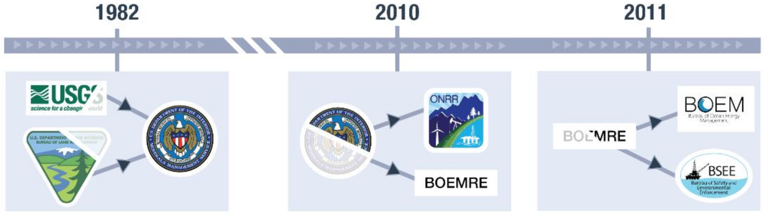
1.1. Historical Perspective

DOI’s U.S. Geological Survey (USGS) developed the foundation of OSRA in the 1970s to support the OCS leasing program [10,11,12]. At that time, DOI’s Bureau of Land Management (BLM) managed the OCS leasing program and environmental assessments using a system similar to land-based leasing within the OCSLA legal structure [13]. USGS performed the estimation of potential petroleum resources and the scientific foundation of spill risk analysis in the environmental assessments. Scientists at USGS determined that a stochastic oil spill trajectory calculation would be the most appropriate for estimating the potential effects of hypothetical large oil spills [10]. In addition, an estimate of the probability of oil spill occurrence coincident to holding a lease sale was made based on historical spills. The combined analysis of the trajectories and the spill probability was renamed OSRA [12]. In 1982, DOI created the MMS by combining elements of BLM and USGS (Figure 1). Following the DWH oil spill, MMS was reorganized into three Bureaus: Office of Natural Resource Revenue (ONRR); BOEM; and Bureau of Safety and Environmental Enforcement (BSEE).

OSRA utilizes a mapped coastline marking the location of critical onshore and offshore environmental resources or resource habitats. The trajectories of the hypothetical spills are calculated using a spatially gridded time series data of ocean currents, surface winds, and sea ice, where applicable. After all of the trajectories have been calculated, the probability of contact to each resource, weighted by the probability of a spill occurring, is estimated [12].

In the late 1970s and early 1980s, studies were funded to investigate seasonal circulation in coastal areas proposed for leasing using diagnostic methods, incorporating climatological observations of temperature, salinity, and ship drift [14,15,16]. The results of those studies allowed estimated climatology of currents to be replaced with fields of ocean surface currents. The ocean currents used prior to the fully dynamic, three-dimensional ocean models were either climatological “maps” of currents or “diagnostic method” currents, which were based on temperature and salinity climatologies.

The dynamic model currents were not used until the assimilation of the satellite altimeter data [17]. The advent of satellite ocean altimeter observations improved the dynamic ocean model estimates by assimilating the altimeter data to nudge the location of the Loop Current, Loop Current Eddies and the Gulf Stream to the appropriate positions. Additional studies produced updated dynamic ocean model results for use in the OSRA model [18,19,20,21,22,23,24,25]. A review of the MMS’s physical oceanography studies and the OSRA model was performed in NAS report in 1990 [26]. Most of the recommendations in the NAS report were adopted in the 1990s.

The environmental studies supporting oil spill modeling have included: (1) physical oceanography and ocean circulation modeling; (2) improved methods of oil spill probability estimation; (3) improved methods of trajectory analysis; and (4) temporal and spatial representations of environmental and socioeconomic resources within and adjacent to OCS areas.

Among field observational studies, the Louisiana–Texas Shelf Physical Oceanography Program ([27]) studied the shelf and shelf break circulation and included hydrographic surveys, ocean moorings, river plume samplings, and satellite observations of the Loop Current and Loop Current Eddies [28,29,30,31,32]. The Surface Current and Lagrangian-Drift Program I & II used primarily surface drifting buoys to improve the understanding of statistical properties of the northern GOM [33].

Results of these studies have been incorporated into OSRA primarily as (1) increased resolution and accuracy of the ocean and atmospheric fields that are used to calculate the oil spill trajectories, and (2) improved detail to the resources that could be impacted.

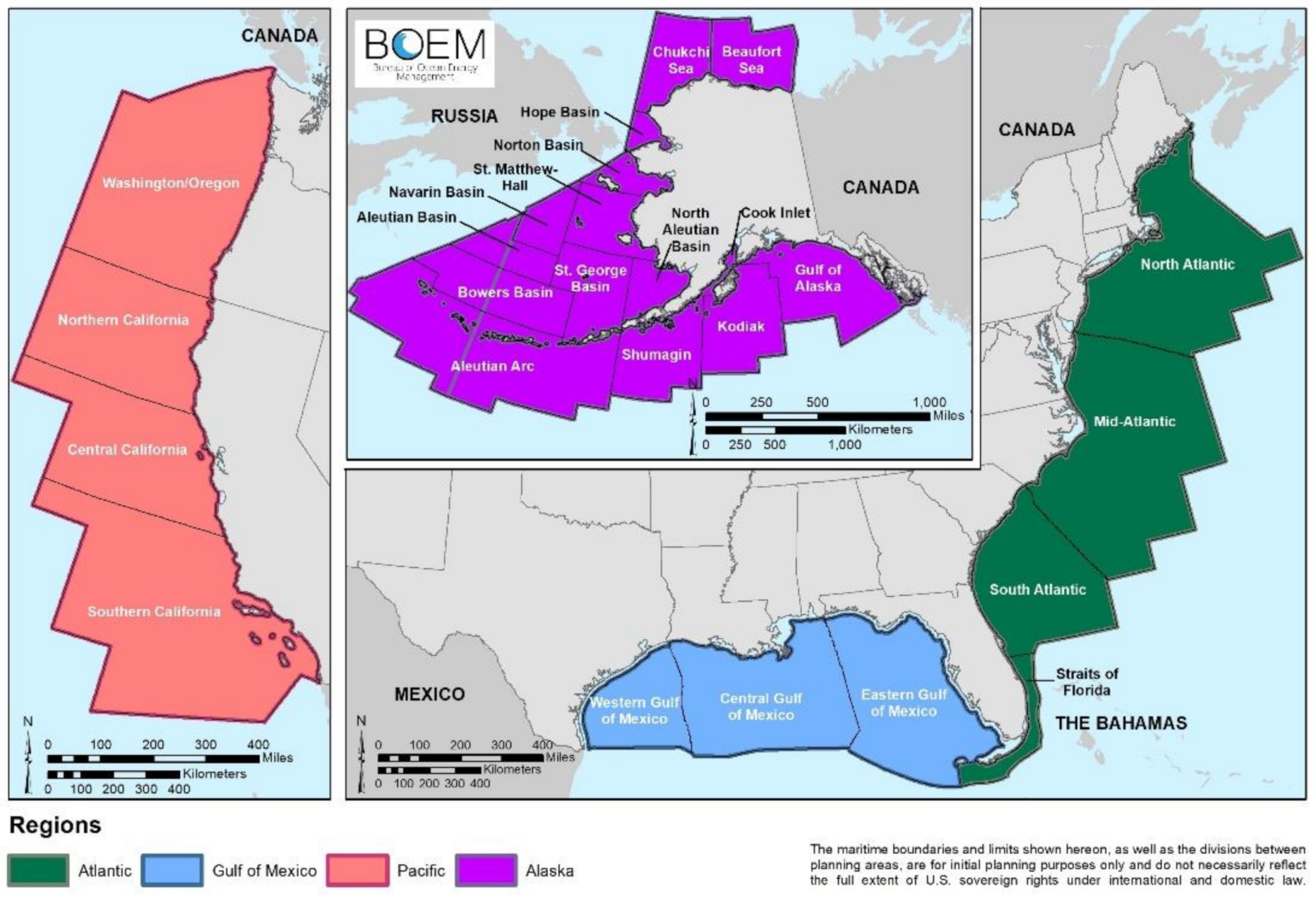
2. Geographic Scope and Scientific Focus of BOEM’s ESP

As shown in Figure 2, the U.S. OCS is divided into four regions: Alaska, Pacific, GOM, and Atlantic. BOEM’s corresponding regional offices are responsible for managing the development of energy and mineral resources on each OCS area. As of March 1, 2021, approximately 12.5 million OCS acres managed by BOEM were actively leased for oil and gas development [34]. In 2019, OCS resources provided about 16% of the Nation’s oil production and almost 3% of domestic natural gas production [35].

3. Summary of BOEM’s Oil Spill Modeling and Physical Oceanographic Studies

This section will highlight BOEM’s studies on advancing oil spill modeling and physical oceanography in the four OCS regions since the DWH oil spill. Studies include field observations of ocean currents and sea ice, numerical modeling of ocean circulation and sea ice, oil spill modeling, and oil spill transports and fates. Studies evaluating the impact of oil spills are not included in this discussion.

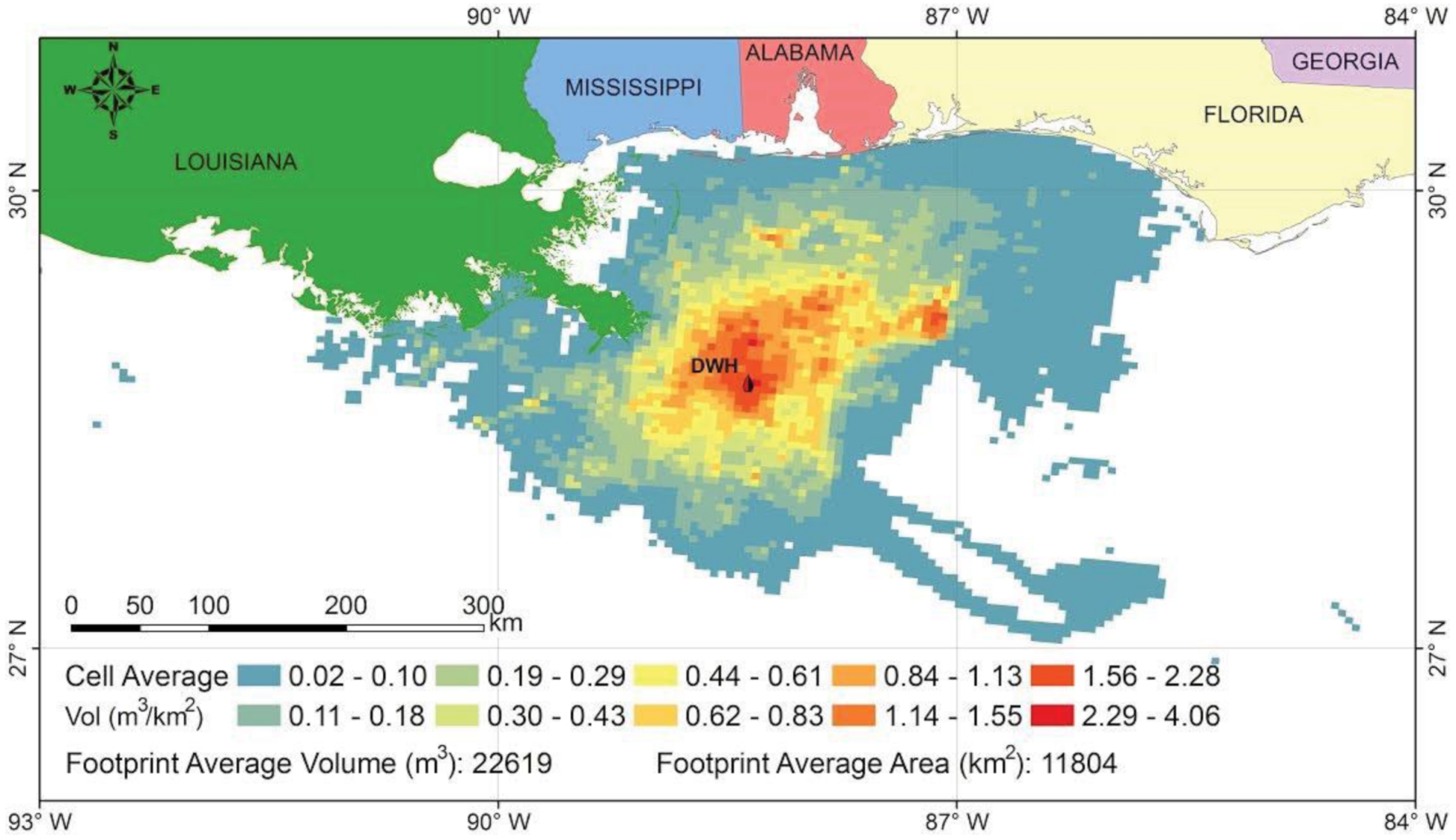
3.1. Gulf of Mexico OCS

Over the last 10 years, BOEM completed 10 oil spill modeling-related studies in the GOM OCS, totaling $9.8 million, of which $7.2 million was spent on physical oceanography and $2.6 million on oil spill modeling (See

Table 1. Summary of ESP studies supporting Oil Spill Modeling (OSP) and Physical Oceanography (PO), including numerical simulations, field observations and sediment transports in the GOM since the DWH oil spill.

No.	Title	Duration	Type	Website & References
1	Data Assimilative Hindcast for the Gulf of Mexico for Oil Spill Risk Analysis	2012/08/17–2015/08/03	PO	27301; [36]
2	A Study to Improve Oil-Spill Risk Analysis in the Gulf of Mexico: A Multi-Model Approach	2012/08/27–2017/08/24	PO	14539; [37]
3	Update to the BOEMRE Oil Spill Risk Analysis (OSRA) Model: Applying Lagrangian Stochastic Model to Track Oil Spills	2010/10/01–2014/02/01	PO	23175; [38]
4	Lagrangian Study of the Deep Circulation in the Gulf of Mexico	2010/10/04–2017/01/20	PO	100029; [39,40,41,42,43,44]
5	A Critical Real-Time Louisiana Coastal Ocean Observing Station	2015/10/01–2019/09/30	PO	1000148; [45,46,47]
6	Simulation Modeling of Ocean Circulation and Oil Spills in the Gulf of Mexico	2011/10/01–2017/08/01	OSP	100032; [48,49,50,51,52,53,54,55,56]
7	Oil/Disbursed Oil-Sediment Interactions in Deepwater Environments	2012/06/01–2016/10/31	OSP	100035; [57,58,59,60,61,62,63,64,65,66,67,68,69,70,71,72,73,74]
8	Remote Sensing Assessment of Surface Oil Transport and Fate During Spills in the Gulf of Mexico	2012/08/27–2017/08/24	OSP	100036; [75,76,77,78,79,80,81,82,83,84,85,86,87,88,89,90,91]
9	Evaluation of the Use of Chemical Dispersants in Oil Spill Response	2017/06/15–2020/03/31	OSP	100211; [8]
10	Shelf-Slope Sediment Exchange in the Northern Gulf of Mexico: Application of Numerical Models for Extreme Events	2011/11/15–2015/08/30	PO	27010; [92,93,94,95]
11	Oil in the Sea IV: Inputs, Fates, and Effects	2020/04/01–2022/03/31	OSP
12	High Resolution Modeling of the Gulf of Mexico	2020/09/23–2023/09/22	PO

Note: For website information, the hyperlink provides the corresponding webpage in ESPIS, e.g., 2730127301 represents the web address https://marinecadastre.gov/espis/#/search/study/27301 (accessed on 5 April 2021).

). These studies generated 12 technical reports and 48 peer-reviewed journal articles.

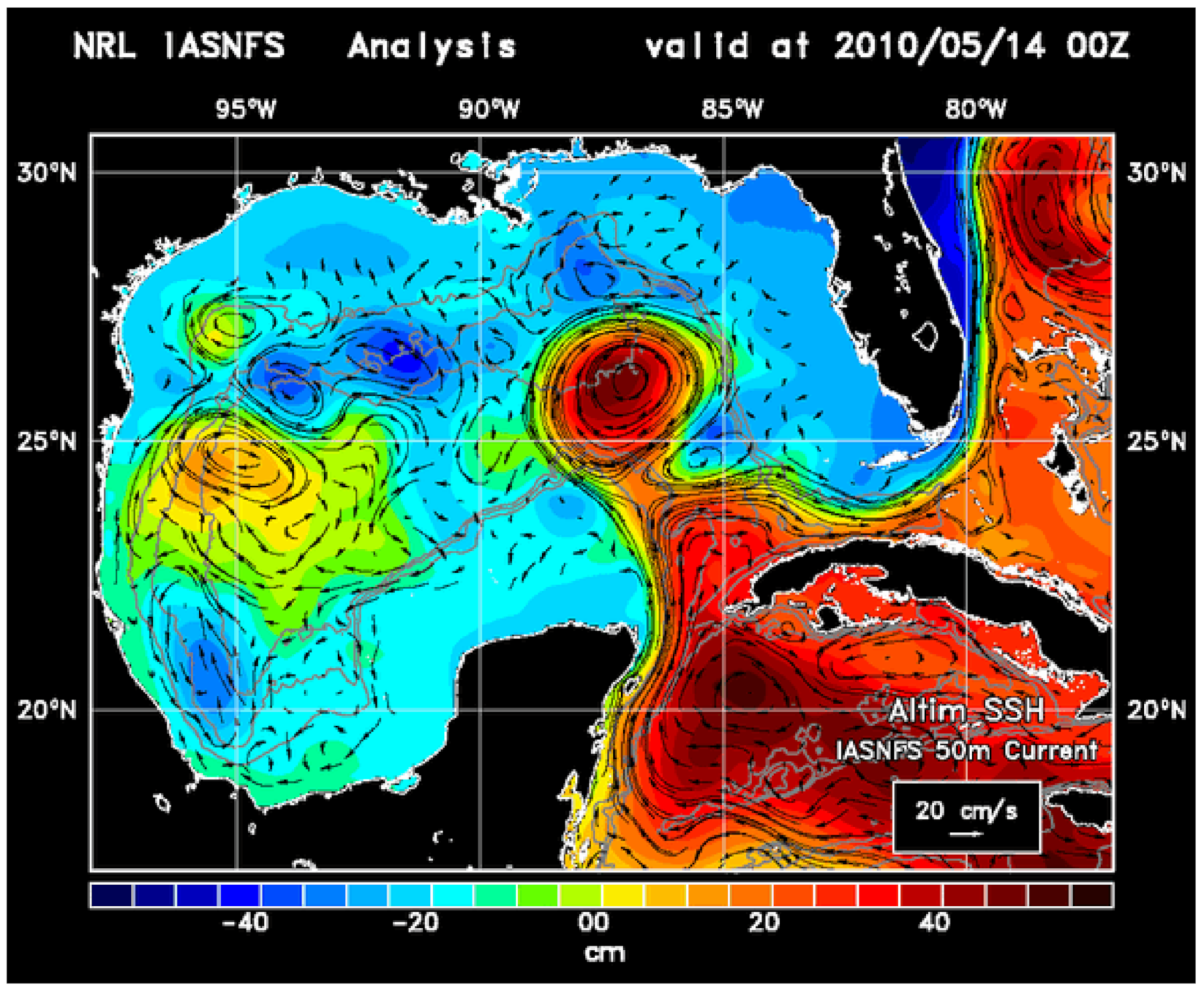
3.1.1. Numerical Simulations

To estimate the spill risk associated with oil and gas development in the GOM OCS, the high-resolution gridded products of surface currents and winds in the GOM are needed to drive an oil spill trajectory model. After the DWH oil spill, BOEM funded two numerical modeling studies [36,37] to simulate ocean circulations in the GOM. The goal was to improve the accuracy of the OSRA for the projected areas of OCS operations and provide more accurate information to BOEM on the oil spill risk management and contingency planning in the GOM.

In 2012, BOEM initiated a numerical modeling study titled Data Assimilative Hindcast for the Gulf of Mexico Oil Spill Risk Analysis with Florida State University (FSU) to produce a high-resolution (in space and time) dataset of ocean state variables from 2003 to 2012 [36]. The latest version of the HYbrid Coordinate Ocean Model (HYCOM) and an ensemble-based data assimilative framework were used to estimate the ocean state variables necessary for OSRA. The model data include three-dimensional ocean currents, temperature, and salinity at hourly intervals.

A parallel numerical modeling study through an Interagency Agreement with the Naval Research Laboratory delivered a ten-year reanalysis of sea surface height (SSH), ocean current, sea temperature, and salinity for the GOM to support this effort [37]. The model output is from the Navy Coastal Ocean Model (NCOM) for the period 2003–2012 in the GOM (Figure 3). The NCOM has been adapted to run in real-time for the Intra-Americas Sea Ocean Nowcast/Forecast System (IASNFS) since 2003. The IASNFS covers the GOM, Caribbean Sea, and Straits of Florida.

In support of BOEM’s policy of using the best available information for safe operations and environmental protection, BOEM has explored new methodologies to improve statistical estimates for OSRA. As mentioned earlier, ocean currents are one of the most critical inputs to OSRA, and the eddy-permitting ocean model cannot resolve the submesoscale (SMS) ocean currents (i.e., motions at the spatial scale of 100 m to 10 km and time scale of a few days). Thus, BOEM contracted with the University of Miami to correct the surface Lagrangian transport by applying Lagrangian stochastic models (LSM) in the SMS range with Lagrangian coherent structures from the eddy-permitting ocean model in the mesoscale range [38]. This study enhanced the scale-dependent relative dispersion of a HYCOM 1/25° simulation from the small scale of about 1 km to twice the scale of the baroclinic radius of deformation, while preserving the relative dispersion at the larger scales. The University of Miami team developed three LSMs that were adapted to the GOM region to estimate the dispersion events at the submesoscale time scales, as these processes play a critical role in the transport of oil spills and other pollutants.

3.1.2. Field Observations

Understanding the patterns of the circulation in the GOM is critical for the successful management of natural resources and the response to accidental oil spills [96]. The ESP-funded studies have significantly improved our understanding of the physical oceanography in the GOM, as summarized by Lugo-Fernández and Green [5]. Beginning around 2001, as oil and gas infrastructure was being installed in deeper waters, BOEM began funding studies to understand the circulation patterns at greater depths. The findings indicate that circulation in the GOM is a two-layered system, a clockwise circulation in the upper layer, and a counter-clockwise circulation in the lower layer.

In 2010, BOEM funded the Lagrangian Study of the Deep Circulation in the Gulf of Mexico project, where a total of 186 floats were deployed over two years, including underwater (RAFOS) floats at depths of 1500 and 2500 m and autonomous profiling (APEX) floats to observe the deep circulation in the GOM [39]. A total of 194 location/velocity and 597 profiles of conductivity, temperature, and depth (CTD) and bio-optical data were obtained, resulting in unprecedented observations of deep circulation throughout the basin in a single four-year interval (2011–2015). The study revealed that there is no deep mass exchange from the eastern to the western basin and also identified new features in the less-studied, deep western basin—an anticlockwise current moving along the escarpment from south of the Mississippi delta, along the Mexican slope, and around the Bay of Campeche to the northeastern point of the Campeche-Yucatan shelf and a cyclonic gyre in the abyssal plain named the Sigsbee Abyssal Gyre. In the eastern GOM, very high eddy kinetic energy was observed [44]. The mesoscale processes were studied by analyzing the RAFOS float trajectory data which revealed a new formation region for anticyclonic eddies off the Campeche Escarpment, located northwest of the Yucatan Peninsula [42]. These eddies seem to be locally formed and are likely to drift westward along the northern edge of the Sigsbee Abyssal Gyre.

The offshore real-time observation of the meteorological and oceanic data in the GOM is critical for supporting BOEM’s mission. In 2015, BOEM funded a project to develop new technology (by reducing the size of the satellite antenna and eliminating onsite computer and cooling systems on the instrument) to establish a new real-time coastal observing station outside coastal Louisiana’s Terrebonne-Timbalier Bays [47]. This was the only real-time station at the time for measuring the current velocity in the Gulf Coast Ocean Observing System network, which collected more than 10 months of real-time data.

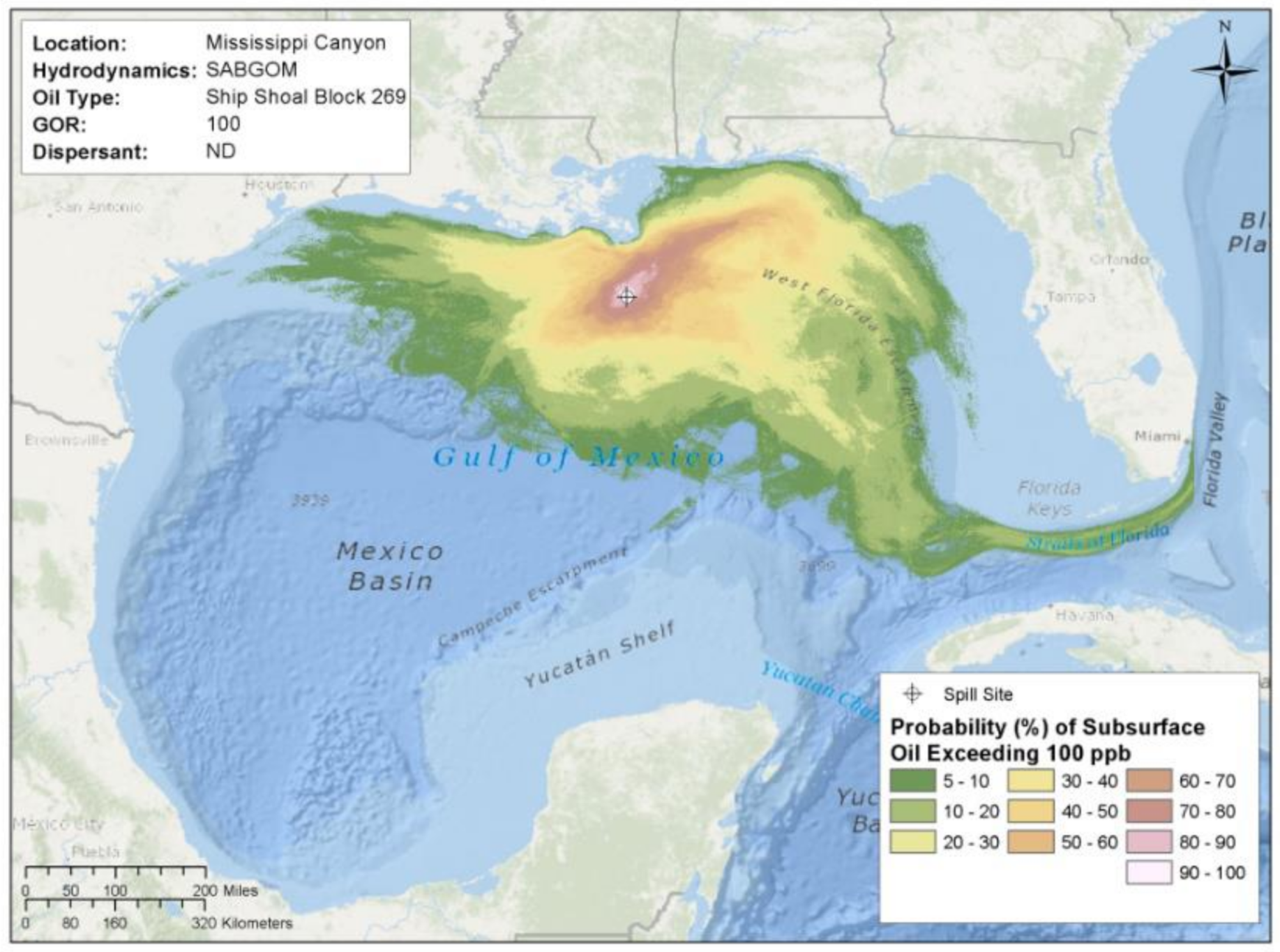
3.1.3. Oil Spill Modeling

Shortly after the DWH oil spill, BOEM initiated the project Simulation Modeling of Ocean Circulation and Oil Spills in the Gulf of Mexico to investigate the effects of oil releases from various depths and locations within the GOM [53,54,55]. The primary objective was to develop and apply an oil spill model that incorporates the processes responsible for oil transport and fate unique to deep oil spills. To accomplish this, the Spill Impact Model Application Package (SIMAP) oil transport and fate model was chosen to simulate spills and perform spill risk assessments. Over the years, SIMAP had undergone extensive testing and code verification to ensure each algorithm was operating as expected and was consistent with the underlying theoretical framework. This work was carried out under a separate contract with the National Oceanic and Atmospheric Administration (NOAA) and Deepwater Horizon Trustees [97] as part of the Natural Resource Damage Assessment [98]. SIMAP was initialized using calculations by OILMAP DEEP (a well-tested blowout model to simulate subsurface oil and gas releases) to simulate the near-field transport of oil and gas discharged from well blowouts and other high-velocity subsurface discharges. The two models received significant enhancements, including a new unified oil droplet size model algorithm [48,49], updated oil weathering algorithms, and newly developed hydrocarbon component-specific degradation rates applicable to GOM surface and deep waters. To better understand the dynamics of a subsea well blowout, field data was collected during the DWH spill event. The results contributed to verifying and improving both trajectory modeling and the fate and effects of oil discharged at depth [52].

Hydrodynamic models quantifying the three-dimensional flow and meteorological model output datasets quantifying the two-dimensional surface wind field in the GOM were collected and reviewed. Gridded profiles of salinity, temperature, and suspended sediment in the water column, as well as geospatial data defining the bathymetry, shoreline, and habitats, were collected and processed into input files for modeling. The physical and chemical properties of the crude oils were collected and used in the blowout model, fate and transport and spill risk assessment. The spill risk assessment included 72 well blowout scenarios representing a range of possible blowout events from sites across the GOM. A blowout model was used to simulate the plume trap height and oil droplet size distribution for a continuous release of 30 days. Results from the blowout model were used in SIMAP to simulate oil spill fate and transport for 75 days. The varied parameters included location of spill, oil type, gas-to-oil ratio, and assumed subsea dispersant effectiveness.

Overall, the model results provide a characterization of potential oil exposure from a 45,000 barrels/day well blowout in different parts of the GOM (Figure 4). The completed integrated system includes data, simulation models, and post processors designed to model the transport and fate of oil from well blowouts in stochastic mode to calculate the spatial and temporal likelihood of oil contamination, and in deterministic mode to predict the trajectory and fate of individual spill events.

Though spilled oil is expected to undergo complex physical, chemical, and biological processes, information was lacking after the DWH oil spill about the interactions among oil, dispersant, and sediment in the marine environment, and how such interactions affect the environmental fate and transport of key oil compounds, such as polycyclic aromatic hydrocarbons (PAHs), n-alkanes, and total petroleum hydrocarbons (TPHs). Thus, BOEM funded a study, Oil and Dispersed Oil-Sediment Interactions in the Marine Environment and Impacts of Dispersants on the Environmental Fate of Persistent Oil Components, which focused on oil n-alkanes, PAHs, three representative dispersants, and three sample coastal sediments from the GOM [72]. The research objectives were achieved through a series of laboratory experiments that focused on: (1) interactions between dispersants, oil and marine sediments and how such interactions affect the environmental transport and transformation of persistent oil components, (2) effects of dispersants on the oil weathering rate due to photochemical degradation and surface-level ozone oxidation, and (3) engineered technologies for enhanced natural weathering of persistent oil components.

The study found that increasing dispersant concentration progressively enhances sediment uptake of PAHs and other oil compounds, and the presence of oil dispersants during desorption results in remarkable sorption hysteresis of PAHs. Sediment organic matter has a key role in sorption of oil, dispersants and dispersed oil. Oil dispersants accelerate the settling rate of suspended sediment particles, and promote formation of marine oil snow, which in turn facilitates transport and distribution of oil in marine ecosystems. The presence of Corexit EC9500A promotes photodegradation of PAHs due to enhanced formation of superoxide or hydroxyl radicals. Methylated PAHs are more prone to photolysis than their parent PAHs. The surface-level atmospheric ozone plays a significant role in oil weathering. The natural photodegradation processes can be further enhanced or supplemented using highly reactive engineered, photocatalysts based, titanate nanotubes; and combined ozonation and photocatalytic degradation show great synergetic effect.

Remote sensing played a key role in detecting oil spilled during the DWH event. Together with the ocean circulation model, remote sensing products can provide crucial information for determining the location and spread of surface oil. BOEM funded a multi-disciplinary project, Remote Sensing Assessment of Surface Oil Transport and Fate During Spills in the Gulf of Mexico, which was led by scientists from FSU, the University of South Florida, and the Norwegian Technical and Industrial Research Institute—Stiftelsen for Industriell og Teknisk Forskning (SINTEF). As shown in Figure 5, the researchers completed a comprehensive and technically innovative analysis of synthetic aperture radar (SAR) and optical remote sensing images of the DWH oil spill and of lesser discharges from natural and anthropogenic sources [87]. Their work improved the detection methods of floating oil and understanding of the environmental effects (e.g., winds and currents) on spreading and dissipating surface oil slicks. Additionally, they demonstrated the differences between the “actual surface current” and the velocity from the surface layer of the ocean model. The understanding of near-surface physics could lead to improvements in simulating oil spills, as the actual surface current is likely substantially greater than the surface velocity simulated by the ocean circulation model. In this study, SINTEF’s Oil Spill Contingency and Response(OSCAR) model was adapted to simulate the dispersion and fate of the surface oil during the DWH event.

Additionally, BOEM sponsored synthesis efforts focused on oil spill science, leading to the completion of the NASEM report titled The Use of Dispersants in Marine Oil Spill Response [8] in 2019.

3.1.4. Sediment Transport

To improve offshore safety and reduce adverse effects of oil spills, BOEM funded a large modeling study to enhance understanding of sediment transport dynamics in the northern GOM. This information is needed because the two largest oil spills in U.S. OCS waters showed that not only can an oil spill be caused by a sudden high-energy, sediment transport event (as in the Taylor platform spill in Mississippi Canyon block 20 [99]), but also that oil can mix with sediments on the seafloor and be transported to distant locations (which occurred during and after the DWH spill [100]). The Taylor platform spill is the largest hurricane-induced oil spill to occur (in terms of volume) in U.S. OCS waters that was generated by gravity currents [101] flowing down a sloping bottom. These currents were induced by the passage of Hurricane Ivan [102] in 2004. The vast majority of sediment transport studies use different types of modeling approaches [103,104,105] while sparse observations are commonly used to validate model solutions [106] and infer past activity from the geological record [107]. For BOEM, this and other information is of great value as it is often used to prepare mandated environmental documents later used to inform leasing and other decisions.

In mid-2010, right after the DWH spill, BOEM started planning a major sediment transport modeling study in the GOM [95]. A partnership among four universities and a modeling center (funded by the U.S. National Science Foundation) conducted this study. The researchers found that wave resuspension of sediments on the shelf generated intermittent sediment fluxes down the DeSoto and Mississippi Canyons after peak atmospheric forcing. This led to the identification of a time lag of about five days between maximum atmospheric forcing at the coastline and maximum offshore sediment transport down the slope at those and other locations. This finding was of great importance because this lag is very similar to the observed lag (about four days) between the time the Taylor platform was toppled by gravity currents and maximum sea level rise at the shoreline [95]. It is speculated here that the relaxation process that followed the maximum storm surge at the coastline (maximum sea level rise) not only enabled offshore flows, but it also led to the sedimentation of previously re-suspended sediments, thus enhancing the sediment load after waters returned to calmer conditions on the continental shelf.

Harris et al. (2020) [95] quantified the contributions made by different atmospheric events to sediment transport from the shelf to the slope area. They noted that hurricane conditions from two events, despite only lasting for a few days, accounted for about 30% of the sediment delivered from the continental shelf to the slope in one year. They also found that delivery of sediment due to settling from the freshwater Mississippi River plume at the canyon head or over the continental slope provided a more gradual source of sediment delivery from October 2007 to September 2008. The remaining 70% was accounted for by plume delivery and transport during the moderate intensity frontal passage, a common occurrence during the spring season in the northern GOM. Significant movement of sediments can, therefore, lead to oil spills by toppling oil platforms and breaking pipelines, and they can also form oil-sediment mixes that get transported away from the contact area. Although major sediment transport takes place only during strong atmospheric events or very large Mississippi River discharge episodes, it is important to better understand how different types and sizes of sediments are displaced in the northern GOM. It is well-known that this high-energy and sudden transport of sediments can negatively impact benthic communities [108,109] as well as coastal resources [110] that are distantly located from the spill site. The damage could be more detrimental to these communities if oil is present in the transported sediments.

In 2019, BOEM started a Federal-academic partnership, the Offshore Analysis of Seafloor Instability and Sediments, to target common and complementary goals focusing on high-energy sediment transport events in the GOM and their potential impacts on offshore infrastructure, human safety, and benthic communities. This group takes into account that these large seafloor instability events, in the form of gravity currents, are more common than previously thought [111,112]. These events have been able to displace archaeological cultural resources lying on the seafloor a few hundreds of meters from their original location (Melanie Damour, personal communication). Monitoring the exact location of these resources is of fundamental importance because they need to be protected from diverse activities ranging from drilling to tourism. These seafloor instability events can also generate important changes in water depth, leading to changes affecting sound propagation [113], a key aspect impacting underwater communications for humans and marine mammals. Improving our understanding of gravity currents (in general) and turbidity currents (in particular) would pave the way for more sustainable decisions on offshore energy, e.g., leasing in or near areas with a recent history of instability events. A better understanding of sediment transport physics (e.g., resuspension and deposition) as well as the response to different forcing mechanisms, will aid in addressing environmental concerns related to the discharge of produced waters from oil platforms [114].

Looking forward, it is important to anticipate and prepare for seafloor instability events, as well as to systematically use research findings and monitoring networks to manage the socio-ecological system on the U.S. OCS [115]. Future work will require improving model parametrizations and increasing surveys in areas prone to the presence of powerful gravity currents. Two main tasks need prompt attention from the community: the inclusion of two-way interactions in multi-model workflows ([95]) and the better representation of turbidity currents in current models [116]. Combining results from Direct Numerical Simulations, Large-Eddy Simulations and Reynolds Averaged Navier-Stokes models have the potential to advance the community’s understanding of turbidity currents, as shown in [117].

3.1.5. Ongoing Studies

BOEM is currently supporting NASEM on developing the synthesis report Oil in the Sea IV: Inputs, Fates, and Effects. This project aims to update the previous report (Oil in the Sea III: Inputs, Fates, and Effects, 2003 [118]) and will provide the state-of-the-science assessment on the fate and effects of oil in the marine environment.

BOEM is continuously seeking better and more accurate information on currents and eddy activities in the GOM. A study on high resolution modeling of the GOM was recently awarded to FSU on enhancing the HYCOM with a high grid resolution of 1/100°. This study will provide BOEM with 20 years of hindcast oceanographic data for use in OSRA applications.

3.2. Alaska OCS

In the last decade, Alaska ESP studies sought to incrementally improve coupled sea ice-ocean and sea ice models; collect oceanographic and sea ice data; conduct oil fate and weathering experiments; and analyze the causal factors and frequency of oil spills. Funding these four areas of research has improved inputs to the OSRA and SINTEF oil weathering models and provided understanding and verification of physical processes and features on the Alaska OCS. The ESP funded 21 studies in these four general areas of research totaling approximately $18 million (

Table 2. Summary of ESP studies supporting oil spill modeling in Alaska since the DWH event.

No.	Title	Duration	Type	Website & References
1	Development of a Very High-Resolution Regional Circulation Model of Beaufort Sea Nearshore Areas	2015/07/24–2018/07/07	NM	100076; [119,120,121]
2	Cook Inlet Circulation Model Calculations	2013/12/17–2016/10/31	NM	26920; [122,123,124]
3	Development of an Accurate Model of the Beaufort and Chukchi Ice Drift and Dispersion for Forecasting Spill Trajectories and Providing Decision Support for Spill Response	2013/05/02–2017/07/24	NM	26899; [125,126]
4	Chukchi Acoustic, Oceanography and Zooplankton Study: Hanna Shoal (CHAOZ, CHAOZ-X including Arctic Whale Ecology Study (ArcWEST)	2014/10/01–2017/08/01	PO	26890; [127,128,129,130,131]
5	Chukchi Offshore Monitoring in Drilling Area (COMIDA) Hanna Shoal Ecosystem Study	2011/09/20–2017/08/31	PO	26833; [132,133,134]
6	Development and Testing of a Low-Cost Satellite-Tracked Ice Drifter for Arctic Alaska	2016/04/02–2018/05/01	PO/FW	26908; [135]
7	Synthesis of Arctic Research (SOAR) Physics to Marine Mammals in the Pacific Arctic	2011/05/13–2018/06/15	S	20001; [136,137,138,139]
8	Satellite-Tracked Drifter Measurements in the Chukchi and Beaufort Seas	2011/04/01–2015/04/15	PO	27208; [140]
9	Characterization of the Circulation on the Continental Shelf Areas of the Northeast Chukchi and Western Beaufort Seas	2012/08/16–2018/01/30	PO	26869; [141,142,143,144,145,146,147]
10	Marine Arctic Ecosystems Study (MARES) Pilot Program Task 3; Biophysical and Chemical Observations	2015/04/24–2018/04/23	PO	100232; [148,149,150]
11	Arctic Tracer Release Experiment (ARCTREX) Applications for Mapping Spilled Oil in Arctic Waters	2013/08/19–2017/12/30	PO/FW	26872; [151]
12	Crude Oil Infiltration and Movement in First-year Sea Ice: Impacts on Ice-associated Biota and Physical Constraints	2014/04/21–2017/07/14	FW	26905; [152,153]
13	Microbial Biodegradation of Alaska North Slope Crude Oil in the Arctic Marine Environment	2017/10/01–2020/06/30	FW	100198; [154,155]
14	Fate and Persistence of Oil Spill Response Chemicals in Arctic Seawater	2015/05/19–2017/05/14	FW	100129; [156,157]
15	Biodegradation and Transport of Crude Oil in Sand and Gravel Beaches of Arctic Alaska	2014/05/19–2015/07/31	FW	26917; [158,159]
16	Physical and Chemical Analyses of Crude and Refined Oils: Laboratory and Mesoscale Oil Weathering	2014/10/01–2016/09/30	FW	26923; [160]
17	Updates to the Fault Tree for Oil-Spill Occurrence Estimators Needed Under the Forthcoming BOEM 2012–2017, 5-Year Program (2011–2016)	2011/10/01–2016/09/30	OE	23172; [161,162,163,164,165,166]
18	Loss of Well Control Occurrence and Size Estimators for the Alaska OCS	2011/10/01–2014/09/24	OE	14552; [167]
19	Updates to the Fault-Tree for Oil Spill Occurrence Estimators (2017–2022)	2017/09/25–Present	OE	100225; [168,169,170]
20	Oil Spill Occurrence Estimators for Onshore Alaska North Slope Crude and Refined Oil Spills	2010/10/01–2015/09/30	OE	23173; [171,172]
21	Oil Spill Occurrence Estimators for Onshore Alaska North Slope and Cook Inlet Crude and Refined Oil Spills	2018/10/02–2021/03/31	OE	100240; [173,174]

Note: For website information, the hyperlink provides the corresponding webpage in ESPIS, e.g., 10076, represents the web address https://marinecadastre.gov/espis/#/search/study/100076 (accessed on 20 July 2020). Key: NM = Numerical Modeling, PO = Physical Oceanography, CR = Cryosphere, S = Synthesis, OE = Occurrence Estimator.

). These studies generated 29 technical reports and 25 peer-reviewed journal articles.

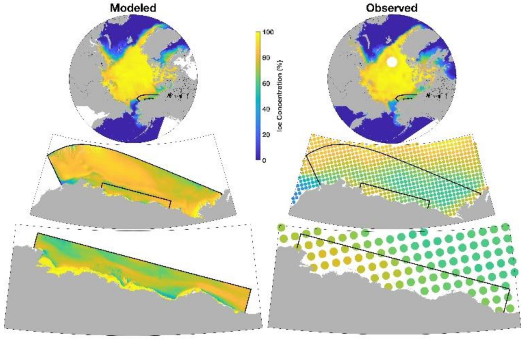
3.2.1. Numerical Simulations

Three numerical modeling studies have been conducted since 2010 (Table 2). The OSRA trajectory simulations for Alaska used output from Rutgers University’s Regional Ocean Modeling System (ROMS) coupled sea ice-ocean model for both the nearshore Beaufort Sea and northwestern Gulf of Alaska, including Cook Inlet. Hindcasts for current, ice velocity, coverage, and thickness were produced using meteorological forcing from available reanalysis data. Incremental improvements to underlying model processes included adding wetting and drying in Cook Inlet, increasing model resolution, and improving estimates of bathymetry, coastal discharge, and landfast ice parameterization.

The ROMS model was set up for the Beaufort Sea as a Pan-Arctic model, a nested regional Beaufort model, and a nested Beaufort shelf model. The nested approach successfully demonstrated the ability to integrate the circulation and sea ice dynamics in the region of interest at a very high resolution for decadal timescales. The nominal resolution of the models was roughly 6 km for the area of interest and coarsening elsewhere for the Pan-Arctic, roughly 3 km curvilinear resolution regionally, and a 0.5 km resolution over the nearshore coastal Beaufort. Simulations were carried out 17 years (1999–2015). Improvements in the nearshore Beaufort Sea included increasing resolution, updated bathymetry, landfast ice parameterization to simulate the formation and breakup of landfast ice, warm river sources and flow, sea ice boundary conditions, and climatology nudging [119,122,175]. Landfast ice parameterization [176] added a large bottom stress to the ice when the estimated keel depth approaches that of the water column. This resulted in a landfast ice field that grew and contracted with changing wind, ice, and oceanographic conditions (Figure 6).

Lu et al. (2020) [121] used an idealized ROMS simulation for a portion of the Chukchi Sea called the Central Channel. They used a series of analyses to investigate the effects on ice ablation of wind, atmospheric fluxes, and the heat and mass flux of Bering Strait flow. These analyses resulted in an organized understanding of how these factors affect ice retreat.

The ROMS model was set up regionally for the Gulf of Alaska at a moderately high resolution (~1.5 km), and simulations were carried out for the ten-year period of 1999–2008. The model evaluation included an analysis of tidal amplitudes, tidal currents, sub-tidal currents, temperature and salinity, and sea ice cover. Advances were implemented in the coastal freshwater forcing for Gulf of Alaska ocean circulation models and the addition of wetting and drying for the dynamic tides in upper Cook Inlet [122,124]. Improvements to the coastal discharge allowed the reproduction of coastal plumes or buoyancy-driven currents.

Kulchitsky et al. (2017) [125] developed a discrete element method (DEM) model of sea ice, Siku, to forecast lead patterns. The DEM was set up with a moderately high regionally-scaled resolution of 2.5 km for the Chukchi and Beaufort Seas, and 25–100 km resolution across the rest of the Arctic Ocean. Simulation results were used to evaluate the physical validity of the proposed physics of ice-ice and ice-coast contact and to compare to lead patterns. The results showed that a simple elastic-brittle model is suitable for modeling the propagation and extent of these leads; however, the results also showed that the model does not adequately simulate the curvature of arches (Figure 7). Lewis and Hutchings (2019) [126] described lead patterns in the Beaufort Sea and identified four general patterns: (1) resulting from tensile failure; (2) associated with shear; (3) coastal flaw; or (4) internal pack, which followed the seasonality in atmospheric pressure systems.

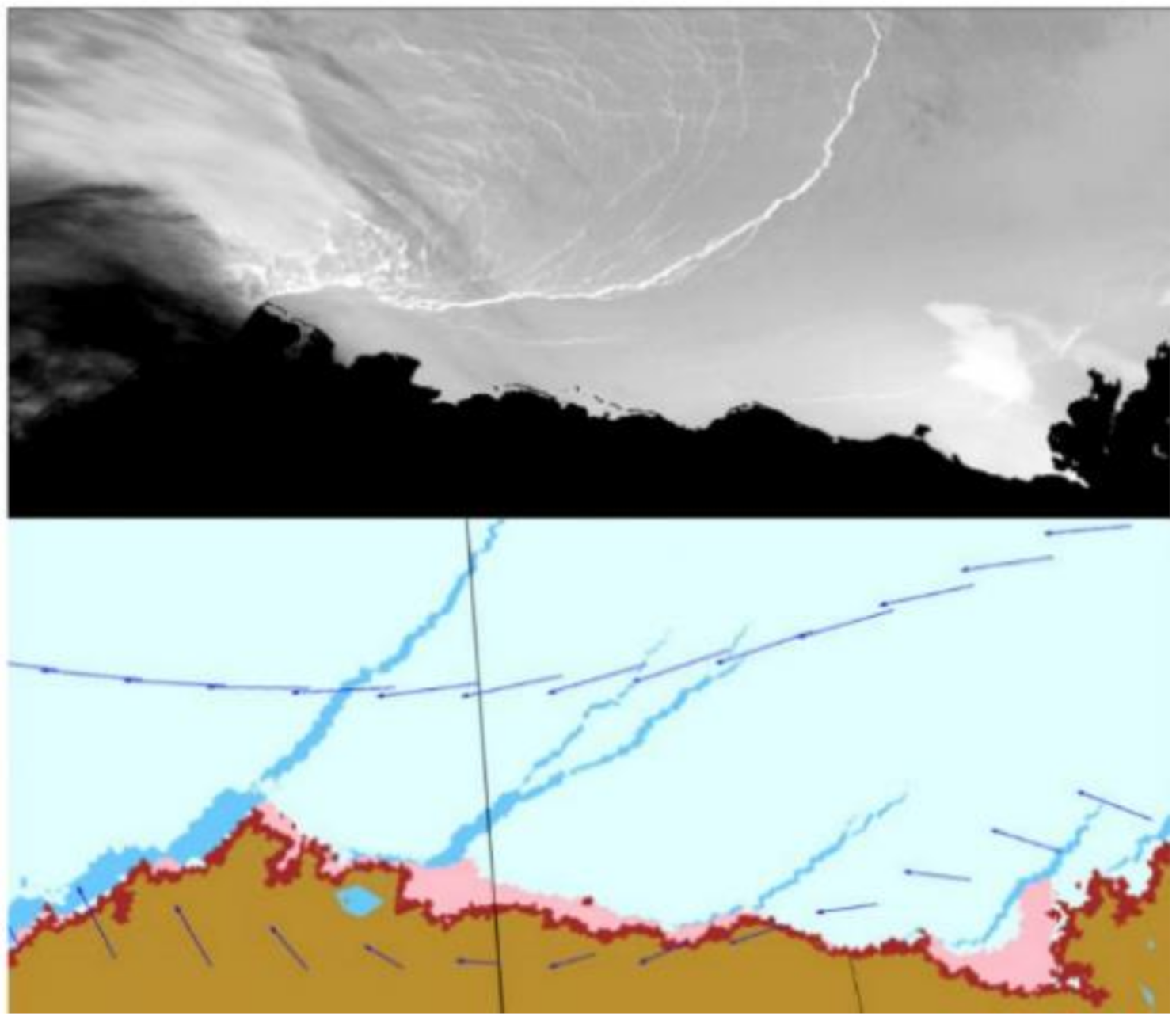
3.2.2. Field Observations

OCS areas adjacent to Alaska are challenging environments for obtaining in-situ oceanographic observations. BOEM partnered with Federal and State agencies, universities, Alaska Native tribes, and industry to leverage scientific opportunities. Table 2 shows several large-scale observational programs including the Chukchi Acoustic, Oceanography and Zooplankton Study (CHAOZ), CHAOZ-Extension (CHAOZ-X), Arctic Whale Ecology Study (ArcWEST), Chukchi Offshore Monitoring in Drilling Area (COMIDA) Hanna Shoal Ecosystem Study, Marine Arctic Ecosystems Study (MARES), and Characterization of the Circulation on the Continental Shelf Areas of the Northeast Chukchi and Western Beaufort Seas. Collectively, these studies refined the understanding of the seasonal circulation and water mass properties on the U.S. Arctic shelf and slope. Observations from these programs and others, listed in Table 2, are used for validation and verification of the hindcast output of coupled ice-ocean circulation models and to provide insight into and improve modeled processes.

From 2012–2014, Weingartner et al. (2017) developed a comprehensive understanding of the physical oceanography in the northeast Chukchi Sea shelf and slope region between the Central Channel and the western Beaufort Sea shelf and slope using a variety of instruments.: moorings; satellite-tracked drifters; towed CTD (acrobat); autonomous underwater vehicles (gliders); shipboard measurements; high frequency radars; and meteorological buoys [144]. This research effort identified the Chukchi Slope current—a subsurface current transporting Pacific-origin water westward over the upper continental slope—and quantified its seasonality [142,146,147]. Major surface current patterns in the northeastern Chukchi, and the wind conditions under which they occur, were derived and mapped [141,143]. The researchers also calculated the seasonal transport (and variations) at the head of Barrow Canyon [145].

From 2011–2013 in the Hanna Shoal portion of the northeastern Chukchi Sea, Dunton et al. (2016) utilized shipboard and towed CTDs, current meters, satellite-tracked drifters, and remotely sensed sea ice data, and found large interannual variations in the hydrographic properties surrounding Hanna Shoal [132]. Further study also provided understanding of the complex interactions of bathymetry, water mass contributions, sea ice, and formation of dense winter water affecting circulation [133]. Circulation patterns showed a general clockwise flow around the north and east sides of Hanna Shoal, as well as on the west flank. Unlike the rest of the shelf, observations east of Hanna Shoal indicated the circulation and hydrography maintained a year-round stratification with westward or northwestward flow in the upper layer and southward flow along the bottom [134].

Moorings, satellite-tracked drifters, and hydrographic surveys collected from 2010–2015 as part of CHAOZ, CHAOZ-X, and ArcWEST supplied new information on currents, transports, and their variability on the eastern Chukchi shelf and slope [127,129,131].

Moorings collected from 2016–2017 as part of MARES elucidated the circulation in the vicinity of Mackenzie Canyon on the Beaufort shelf, its response to wind and ice, and how the topography of the canyon influences it [150]. Wind appeared to be the main driver of shelfbreak and Mackenzie Trough circulation. Furthermore, multi-year variability of summertime winds seemed to affect the structure of the Beaufort Gyre, shelfbreak boundary current, and downstream fate of Mackenzie River water. The shelfbreak jet and the coastal current can change strength and direction on event time scales of days to weeks, and thus the summertime Chukchi and Beaufort shelfbreak jet cannot be assumed to be steady on the interannual timescale [149].

Findings from the Synthesis of Arctic Research (SOAR) enhanced scientific understanding of the relationships among oceanographic conditions and biological resources with an emphasis on the northeastern Chukchi Sea. The outcomes supported an enhanced capability to predict future changes in oceanographic features, such as currents, upwelling, and ice leads [136,137,138,139].

3.2.3. Fate and Weathering Studies

Table 2 shows four oil fate and weathering experiments with the majority focused on the U.S. Arctic. In Alaska, the possible distribution and fate of oil spills includes components of the environment not found in other OCS regions— sea ice and cold temperatures. These two variables affect the behavior, fate, weathering, and transport of oils. Laboratory and mesoscale analyses of six crude and refined oils, including in ice and at lower temperatures, were conducted to maintain a current oil library for use in the SINTEF oil weathering model [160]. Composite Alaska North Slope (ANS) crude oil has been extensively studied but other individual crude and diesel oils, especially low sulfur diesel oils, have not. The physical properties of different oil types determine how they behave and weather and ultimately their fate and interaction with the environment and organisms.

Sharma and Schiewer (2016) [159] investigated the effects of temperature, salinity, and crude oil concentration on biodegradation of oil in Arctic seashore sediments. Their results showed a quick initial removal of hydrocarbons by volatilization, but microbial biodegradation of crude oil was low, especially at the lower temperature. McFarlin et al. (2018) [157] and Gofstein et al. (2020) [154] quantified biodegradation and abiotic losses of ANS crude oil and Corexit 9500 in Arctic seawater mesocosms. They identified microorganisms potentially involved in biodegradation of these substrates using tools based on gene analysis. Oggier et al. (2020) [153] developed a semi-empirical multi-stage oil migration and surfacing model to help predict oil in ice behavior which was guided by results from three sets of ice-tank experiments.

3.2.4. Oil Spill Occurrence Estimates

Estimating the frequency of oil spill occurrence is a separate but related avenue of research needed to support OSRA modeling. Attempts to quantify risks from oil spills, which could occur as random events over two to three decades of OCS exploration, development, production, and decommissioning, benefit from evaluating historical oil spill patterns and trends. Five studies collated oil spill data and evaluated the frequency and causal factors of oil spills using historical data and either statistical regression methods or fault tree modeling (Table 2).

Due to the limited offshore exploration and development in the Arctic OCS, it is difficult to compute oil spill frequencies using the small amount of empirical data from that region. Rather, empirical data on OCS spills from the GOM and Pacific OCS were evaluated using a fault tree method based on modification or addition of causal factors unique to the Arctic OCS- such as lack of fishing, low temperatures, and sea ice-related processes, such as ice gouging or strudel scour [162,165,170].

Information about regional oil spill patterns within or adjacent to Alaska, and their causal factors, was evaluated for the ANS and Cook Inlet [171,172,173,174]. Analyzing regional patterns and trends determines if causal factors or occurrence rates vary between regions.

Of particular interest was the update on offshore loss of well control frequency information through 2011 conducted after the DWH event for offshore regions of the U.S., Canada, and Australia; the North Sea; and other areas with a comparable regulatory regime. This included a collation of associated exposure variable information and a statistical characterization of rare catastrophic blowouts such as Ixtoc in 1979 and DWH in 2010 [167].

3.2.5. Ongoing Studies

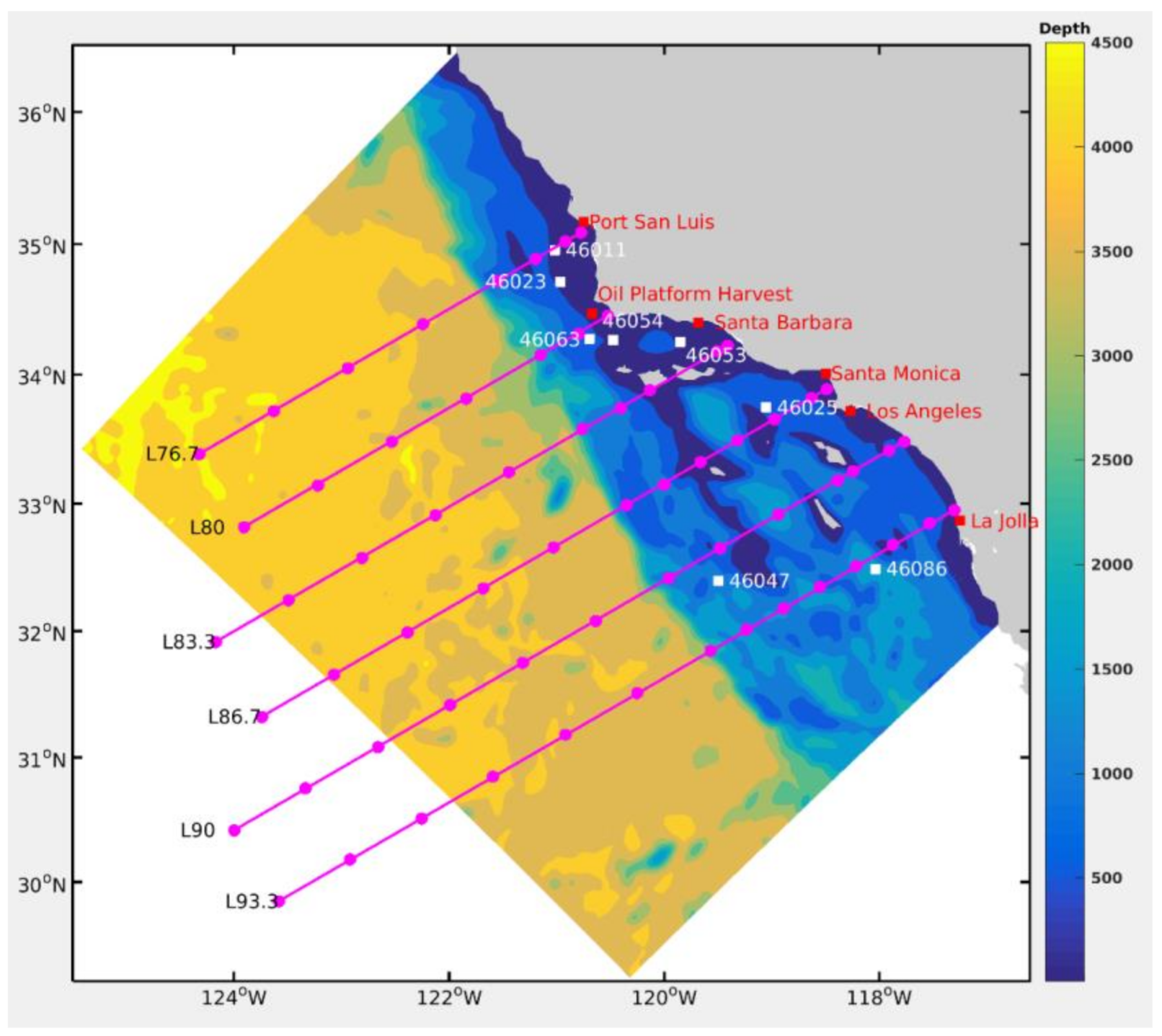
Two ongoing avenues of research include improvements to BOEM’s sea ice modeling by using a new coupled ocean-ice code (i.e., Modular Ocean Model (MOM) version 6 coupled with Community Ice CodE (CICE), known as MOM6-CICE) [177] and characterizing and modeling the wavefield in the nearshore Beaufort Sea [178]. Stefansson Sound and Foggy Island Bay within the Beaufort Sea are difficult to model due to the complex shallow bathymetry and coastal topography, and the highly variable and mobile sea ice conditions. The wavefield study will produce high resolution wave output in the nearshore region of the Beaufort Sea and will collect offshore observations using fixed moorings and buoys for validation.

3.3. Pacific OCS

In the BOEM Pacific Region, the Southern California Planning Area has a mature oil and gas program and has had no new leasing over the past decade. To inform environmental analyses for ongoing operations, BOEM Pacific Region conducts oil spill trajectory modeling as a precaution in the event of a spill from oil and gas facilities in offshore southern California. To improve BOEM’s ability to conduct OSRA offshore southern California, BOEM partnered with the University of California, Los Angeles (UCLA) to conduct a multi-year hindcast (reanalysis) of winds, waves, and currents along the coast of California [179]. BOEM is also partnering with NOAA to utilize the surface currents and winds from UCLA’s ROMS hindcast analysis with the General NOAA Operational Modeling Environment to produce multiple trajectories for NOAA’s Trajectory Analysis Planner (TAP) [180]. Using realistic oil spill scenarios over a range of different regional oceanographic regimes (such as upwelling, relaxation, and eddy-driven flow), TAP will calculate the probabilities of oil contacting parcels of water and shoreline if oil were to spill from southern California platforms. This enables analysts to understand where an oil spill may travel, how long it could take to get there, and the likelihood of spilled oil contacting environmental resources.

The hindcast input to the oil spill models utilized in the BOEM Pacific Region needed to be updated and expanded to provide more accurate information to conduct offshore oil and gas risk analyses over a wider geographic area. The Integrated Ocean Observing Systems along the West Coast of the U.S. maintains real-time observational data of wind, waves, and the currents of offshore coastal California. Reanalysis or hindcast of these observational data enables analysts and decision makers to understand the seasonal and annual variation of wind, waves, and currents. Broadening the geographic range of available data and acquiring, compiling, and converting real-time data through numerical modeling into a format to run oil spill models improved BOEM Pacific Region’s ability to conduct OSRA for southern California. This study applied the Weather Research Forecast, ROMS, and Simulating WAves Nearshore models to provide new ten-year (2004–2013) hindcasts. The model domain extends from just south of Monterey Bay to the Mexican border. The ROMS model has 1 -km horizontal resolution with 42 vertical levels. In this study, hindcast data are validated against observations (Figure 8).

While the UCLA ten-year ROMS hindcast was being developed, BOEM began collaborating with NOAA’s Office of Response and Restoration to develop the TAP study for the Southern California Planning Area. The Southern California TAP utilizes the UCLA ten-year ROMS to force the model. The TAP receptor grid has a 2.5 km horizontal resolution and simulates hypothetical oil spills from the 23 Federal offshore oil and gas platforms (source sites) in the Southern California Planning Area. TAP runs 250 hypothetical spills from each platform for each season (all year, summer, winter) that are initialized at random times during the ten-year period of forcing data. Each oil spill run uses the specific oil type that is produced from each platform and oil particles are weathered along their trajectory, reproducing realistic spill characteristics. TAP has multiple analysis modes to view the oil spill trajectories: impact, oiling, response time, threat, impact by spill, and response time by spill. Impact analysis shows oil spill impact on the receptor grid as the percentage of spills that will affect a receptor cell over a defined limit (spill size). Oiling analysis shows the percentage of oil that will be in a receptor cell. Response time analysis estimates time available to mount a response before oil from a source site will reach each receptor cell. Threat analysis displays the relative threat from each source site at a selected receptor cell. Impact by spill and response time by spill show impact and response time analyses for each of the 250 individual spills from a selected source site. Through this collaboration, NOAA’s Emergency Response Division will develop a web-based TAP viewer to enable this tool to be more flexible and easily available for oil spill response planners and resource evaluators.

3.4. Atlantic OCS

For the Atlantic OCS, BOEM is currently supporting the project Alternative Oil Spill Occurrence Estimators for Determining Rates for the Atlantic Outer Continental Shelf [181]. This study will develop alternative methodologies for determining oil spill occurrence rates of appropriate size for oil and gas activities on the Atlantic OCS, should they be proposed in the future.

4. Conclusions and Outlook

BOEM’s ESP has a long history of supporting research efforts that further our understanding of fundamental physical oceanographic processes and the role they play in the fate and transport of spilled oil. Over the last decade, using a combination of observational tools (moorings, CTDs, satellite-tracked drifters, gliders, high-frequency radars, meteorological buoys, acoustically tracked floats) and numerical models, BOEM’s ESP has sought to fulfill its federal mandate while addressing fundamental scientific questions, such as the deep circulation in the western basin of the Gulf of Mexico and the parameterization of landfast sea ice. BOEM’s funding efforts helped improve algorithms of several leading oil spill models (such as SIMAP and SINTEF’s OSCAR) and contributed significantly to the oil spill modeling community.

Looking ahead, BOEM will continue supporting field observations of ocean currents on the OCS when necessary, while seeking partnerships with other stakeholders. Monitoring and understanding the changes of sea ice in the U.S. Arctic is even more critical as the pace of climate change is accelerating (https://climate.nasa.gov/evidence/ (accessed on 10 December 2020)). BOEM hopes to incorporate results from field observations to improve the parametrization of hydrodynamic models within a five- to seven-year time frame to better support in-house OSRA modeling efforts [182]. The state-of-the-science High Resolution Modeling of the Gulf of Mexico (Section 3.1.5) will likely reveal the submesoscale circulation patterns that are previously undocumented and have few observations to validate model results (Eric Chassignet, personal communication). BOEM will keep funding these numerical modeling studies as they will guide the implementation of field observation programs in the future.

Strategically allocating resources for funding oil spill science will remain important to BOEM’s ESP, particularly as the GoMRI program funding has now ended. Currently, projects are typically initiated on a short-term basis (one- to two- years) corresponding to the ESP study development cycle. Over the long term, BOEM will continue to address strategic science questions for oil spill modeling and related physical oceanography.

Externally, BOEM seeks collaborations with other Federal agencies, especially BSEE. BSEE conducts oil spill response research and tracks oil spill incidents on the OCS. BSEE and BOEM’s 2016 update of oil spill occurrence rates [183] helped support BOEM’s NEPA requirements. BOEM is actively involved in the Interagency Coordinating Committee on Oil Pollution Research, “a 15-member Interagency Committee established by Title VII of the Oil Pollution Act of 1990 (Section 7001) (https://www.dco.uscg.mil/ICCOPR/ (accessed on 10 December 2020))”. BOEM participates in the National Oceanographic Partnership Program (NOPP), which coordinates research priorities in ocean science between Federal agencies to leverage resources for projects that are too large for a single agency to fund or that have overlapping scientific objectives that could benefit from agency collaboration. BOEM is also participating in the Arctic Maritime Spill Response Modeling Working group (https://crrc.unh.edu/amsm-arctic-maritime-spill-response-modeling-working-groups (accessed on 10 December 2020)), which discusses the challenges of modeling oil spills in the Arctic and develops recommendations for addressing modeling needs. BOEM uses these resources to leverage its oil spill modeling efforts and achieve its mission.

References

1. Schleifstein, M. BP and its Partners have Spent $71 Billion over 10 Years on Deepwater Horizon Disaster. Available online: https://www.nola.com/news/business/article_ca773cc0-80f4-11ea-8fbe-ffa77e5297bd.html (accessed on 10 December 2020).
2. The Gulf of Mexico Research Initiative. Available online: https://gulfresearchinitiative.org/ (accessed on 20 July 2020).
3. National Research Council. The Gulf Research Program: A Strategic Vision; The National Academies Press: Washington, DC, USA, 2014. [Google Scholar] [CrossRef]
4. Lugo-Fernández, A. A Temporary Bonanza of Ocean Research Funds in the Gulf of Mexico. Mar. Technol. Soc. J. 2015, 49, 84–87. [Google Scholar] [CrossRef]
5. Lugo-Fernández, A.; Green, R.E. Mapping the Intricacies of the Gulf of Mexico’s Circulation. Eostrans. Am. Geophys. Union 2011, 92, 21–22. [Google Scholar] [CrossRef]
6. Studies Development Plan 2021–2022. Available online: https://www.boem.gov/sites/default/files/documents/environment/environmental-studies/SDP%20FY2021-2022.pdf (accessed on 20 July 2020).
7. Liu, Y.; MacFadyen, A.; Ji, Z.-G.; Weisberg, R.H. Monitoring and Modeling the Deepwater Horizon Oil Spill: A Record-Breaking Enterprise; American Geophysical Union: Washington, DC, USA, 2011. [Google Scholar]
8. National Academies of Sciences, Engineering, and Medicine. The Use of Dispersants in Marine Oil Spill Response; The National Academies Press: Washington, DC, USA, 2020. [Google Scholar] [CrossRef] [Green Version]
9. Ji, Z.-G.; Li, Z.; Johnson, W.R.; Auad, G. Progress of the Oil Spill Risk Analysis (OSRA) Model and Its Applications. J. Mar. Sci. Eng. 2021, 9, 195. [Google Scholar] [CrossRef]
10. Lanfear, K.J. Applications of the USGS Oilspill Trajectory Analysis (OSTA) Model to Decisions Regarding OCS Oil Development. In Proceedings of the Workshop on Government Oilspill Modeling, Wallops Island, VA, USA, 7–9 November 1979; pp. 13–14. [Google Scholar]
11. Samuels, W.B. The USGS Oilspill Trajectory Analysis Model. In Proceedings of the Workshop on Government Oilspill Modeling, Wallops Island, VA, USA, 7–9 November 1979; National Oceanic and Atmospheric Administration, Environmental Data and Information Service: Washington, DC, USA, 1979. 20p. [Google Scholar]
12. Smith, R.A.; Slack, J.R.; Wyant, T.; Lanfear, K.J. The Oilspill Risk Analysis Model of the U.S. Geological Survey. In Geological Survey Professional Paper 1227; United States Government Printing Office: Washington, DC, USA, 1982; p. 40. [Google Scholar]
13. OCS Lands Act History. Available online: https://www.boem.gov/oil-gas-energy/leasing/ocs-lands-act-history (accessed on 27 July 2020).
14. Blumberg, A.F.; Mellor, G.L. A Numerical Calculation of the Circulation in the Gulf Mexico, Report. 66; Dynalysis of Princeton: Princeton, NJ, USA, 1981; 153p. [Google Scholar]
15. Blumberg, A.F.; Mellor, G.L. Diagnostic and Prognostic Numerical Circulation Studies of the South Atlantic Bight. J. Geophys. Res. 1983, 88, 4579–4592. [Google Scholar] [CrossRef]
16. Kantha, L.H.; Mellor, G.L.; Blumberg, A.F. A diagnostic calculation of the general circulation in the South Atlantic Bight. J. Phys. Oceanogr. 1982, 12, 805–819. [Google Scholar] [CrossRef] [Green Version]
17. Mellor, G. Panel recommendations on Oil Spill Risk Assessment. Eos Trans. 1986, 67, 1356. [Google Scholar] [CrossRef]
18. Mellor, G.L.; Ezer, T. A Gulf Stream Model and an Altimetry Assimilation Scheme. J. Geophys. Res. 1991, 96, 8779–8795. [Google Scholar] [CrossRef]
19. Oey, L.-Y. Eddy and wind-forced shelf circulation. J. Geophys. R. 1995, 100, 8621–8638. [Google Scholar] [CrossRef]
20. Oey, L.-Y. Simulation of Mesoscale Variability in the Gulf of Mexico: Sensitivity Studies, Comparison with Observations, and Trapped Wave Propagation. J. Phys. Oceanogr. 1996, 26, 145–175. [Google Scholar] [CrossRef] [Green Version]
21. Herring, H.J.; Inoue, M.; Mellor, G.L.; Mooers, C.N.K.; Niiler, P.P.; Oey, L.-Y.; Patchen, R.C.; Vukovich, E.; Wiseman, J. Coastal Ocean. Modeling Program. for the Gulf of Mexico; U.S. Department of the Interior, Minerals Management Service: Herndon, VA, USA, 1999; p. 539.
22. Wang, D.-P.; Ezer, T.; Oey, L.-Y.; Hamilton, P. Near-Surface Currents in DeSoto Canyon (1997–1999): Comparison of Current Meters, Satellite Observation, and Model Simulation. J. Phys. Oceanogr. 2003, 33, 313–326. [Google Scholar] [CrossRef] [Green Version]
23. Oey, L.-Y. A Wetting and Drying Scheme for POM. Ocean. Model. 2004, 9, 133–350. [Google Scholar] [CrossRef]
24. Lin, X.-H.; Oey, L.-Y.; Wang, D.-P. Altimetry and drifter data assimilations of loop current and eddies. J. Geophys. Res. 2007, 112, C05046. [Google Scholar] [CrossRef] [Green Version]
25. Oey, L.-Y. Loop Current and Deep Eddies. J. Phys. Oceanogr. 2008, 38, 1426–1449. [Google Scholar] [CrossRef]
26. National Research Council. Assessment of the U.S. Outer Continental Shelf Environmental Studies Program: I. Physical Oceanography; The National Academies Press: Washington, DC, USA, 1990; Available online: https://www.nap.edu/catalog/1609/assessment-of-the-us-outer-continental-shelf-environmental-studies-program (accessed on 27 July 2020).
27. Louisiana-Texas Shelf Physical Oceanography Program. Available online: https://www.gulfbase.org/project/louisiana-texas-shelf-physical-oceanography-program (accessed on 22 October 2020).
28. Biggs, D.C.; Fargion, G.S.; Hamilton, P.; Leben, R.R. Cleavage of a Gulf of Mexico loop current eddy by a deepwater cyclone. J. Geophys. Res. 1996, 101, 20629–20641. [Google Scholar] [CrossRef]
29. Li, Y.; Nowlin, W.D.; Reid, R.O. Spatial-scale analysis of hydrographic data over the Texas-Louisiana continental shelf. J. Geophys. Res. 1996, 101, 20595–20605. [Google Scholar] [CrossRef]
30. Murray, S.P. An Observational Study of the Mississippi-Atchafalaya Coastal Plume; OCS Study 98-0040. Obligation No.: 14-35-0001-30632; U.S. Department of the Interior, Minerals Management Service: Herndon, VA, USA, 1998; p. 539.
31. Hamilton, P.; Berger, T.J.; Johnson, W. On the structure and motions of cyclones in the northern Gulf of Mexico. J. Geophys. Res. 2002, 107, 1–18. [Google Scholar] [CrossRef]
32. Nowlin, W.D.; Jochens, A.E.; DiMarco, S.F.; Reid, R.O.; Howard, M.K. Low-frequency circulation over the Texas-Louisiana continental shelf. In Circulation in the Gulf of Mexico: Observations and Models; Sturges, W., Lugo-Fernandez, A., Eds.; American Geophysical Union: Washington, DC, USA, 2005; pp. 219–240. [Google Scholar] [CrossRef]
33. Ohlmann, J.C.; Niiler, P.P. Circulation over the continental shelf in the northern Gulf of Mexico. Prog. Oceanogra. 2005, 64, 45–81. [Google Scholar] [CrossRef]
34. Combined Leasing Report (As of 1 March 2021). Available online: https://www.boem.gov/sites/default/files/documents/about-boem/Lease%20stats%203-1-21.pdf (accessed on 2 April 2021).
35. Oil and Gas Energy: Facilitating the Responsible Development of Oil and Gas Resources on the OCS. Available online: https://www.boem.gov/oil-and-gas-energy (accessed on 22 October 2020).
36. Chassignet, E.P.; Srinivasan, A. Data Assimilative Hindcast for the Gulf of Mexico; OCS Study BOEM 2015-035; U.S. Department of the Interior, Bureau of Ocean Energy Management: Sterling, VA, USA, 2015; p. 46.
37. Ko, D.S.; Wang, D.-P. Intra-Americas Sea Nowcast/Forecast. System Ocean. Reanalysis to Support. Improvement of Oil-spill Risk Analysis in the Gulf of Mexico by Multi-model Approach; OCS Study 2014-1003; U.S. Department of the Interior, Bureau of Ocean Energy Management: Herndon, VA, USA, 2014; p. 65.
38. Haza, A.C.; Ozgokmen, T.M.; Griffa, A.; Ryan, E. Implementation of Lagrangian Stochastic Models to Parameterize Submesoscale Transport. for Tracking Oil Spills in the Gulf of Mexico; OCS Study BOEM 2014-053; U.S. Deptartment of the Interior, Bureau of Ocean Energy Management: Herndon, VA, USA, 2014; p. 70.
39. Hamilton, P.; Bower, A.; Furey, H.; Leben, R.; Pérez-Brunius, P. Deep Circulation in the Gulf of Mexico: A Lagrangian Study; OCS Study BOEM 2016-081; U.S. Department of the Interior, Bureau of Ocean Energy Management: Sterling, VA, USA, 2016; p. 292.
40. Green, R.; Bower, A.; Fernandez, A. First Autonomous Bio-Optical Profiling Float in the Gulf of Mexico Reveals Dynamic Biogeochemistry in Deep Waters. PLoS ONE 2014, 9, e101658. [Google Scholar] [CrossRef] [Green Version]
41. Pasqueron de Fommervault, O.; Perez-Brunius, P.; Damien, P.; Camacho-Ibar, V.F.; Sheinbaum, J. Temporal variability of chlorophyll distribution in the Gulf of Mexico: Bio-optical data from profiling floats. Biogeosciences 2017, 14, 5647–5662. [Google Scholar] [CrossRef] [Green Version]
42. Furey, H.; Bower, A.; Perez-Brunius, P.; Hamilton, P.; Leben, R. Deep Eddies in the Gulf of Mexico Observed with Floats. J. Phys. Oceanogr. 2018, 48, 2703–2719. [Google Scholar] [CrossRef] [Green Version]
43. Hamilton, P.; Leben, R.; Bower, A.; Furey, H.; Pérez-Brunius, P. Hydrography of the Gulf of Mexico Using Autonomous Floats. J. Phys. Oceanogr. 2018, 48, 773–794. [Google Scholar] [CrossRef]
44. Pérez-Brunius, P.; Furey, H.; Bower, A.; Hamilton, P.; Candela, J.; García-Carrillo, P.; Leben, R. Dominant Circulation Patterns of the Deep Gulf of Mexico. J. Phys. Oceanogr. 2018, 48, 511–529. [Google Scholar] [CrossRef] [Green Version]
45. Chaichitehrani, N.; Li, C.; Xu, K.; Allahdadi, M.N.; Hestir, E.L.; Keim, B.D. A numerical study of sediment dynamics over Sandy Point dredge pit, west flank of the Mississippi River, during a cold front event. Cont. Shelf Res. 2019, 183, 38–50. [Google Scholar] [CrossRef]
46. Li, C.; Huang, W.; Milan, B. Atmospheric Cold Front–Induced Exchange Flows through a Microtidal Multi-Inlet Bay: Analysis Using Multiple Horizontal ADCPs and FVCOM Simulations. J. Atmos. Ocean. Technol. 2019, 36, 443–472. [Google Scholar] [CrossRef]
47. Li, C.; Milan, B.; Huang, W.; Luo, Y. A Real-Time Ocean Observing Station Off Timbalier Bay, Louisiana; OCS Study BOEM 2020-015; U.S. Department of the Interior, Bureau of Ocean Energy Management: Sterling, VA, USA, 2020; p. 74.
48. Li, Z.; Spaulding, M.; French-McCay, D.; Crowley, D.; Payne, J.R. Development of a unified oil droplet size distribution model with application to surface breaking waves and subsea blowout releases considering dispersant effects. Mar. Poll. Bull. 2017, 114, 247–257. [Google Scholar] [CrossRef]
49. Li, Z.; Spaulding, M.L.; French-McCay, D. An algorithm for modeling entrainment and naturally and chemically dispersed oil droplet size distribution under surface breaking wave conditions. Mar. Pollut. Bull. 2017, 119, 145–152. [Google Scholar] [CrossRef]
50. Spaulding, M.; Li, Z.; Mendelsohn, D.; Crowley, D.; French-McCay, D.; Bird, A. Application of an Integrated Blowout Model System, OILMAP DEEP, to the Deepwater Horizon (DWH) Spill. Mar. Pollut. Bull. 2017, 120, 37–50. [Google Scholar] [CrossRef]
51. Spaulding, M.L. State of the art review and future directions in oil spill modeling. Mar. Pollut. Bull. 2017, 115, 7–19. [Google Scholar] [CrossRef]
52. French-McCay, D.; Horn, M.; Li, Z.; Jayko, K.; Spaulding, M.; Crowley, D.; Mendelsohn, D. Modeling Distribution Fate and Concentrations of Deepwater Horizon Oil in Subsurface Waters of the Gulf of Mexico. In Oil Spill Environmental Forensics Case Studies; Stout, S., Wang, Z., Eds.; Elsevier: Amsterdam, The Netherlands, 2018; pp. 683–736. [Google Scholar] [CrossRef]
53. Galagan, C.W.; French-McCay, D.; Rowe, J.; McStay, L.; Crowley, D. Simulation Modeling of Ocean Circulation and Oil Spills in the Gulf of Mexico. Volume I: Synthesis Report; OCS Study BOEM 2018-039; U.S. Department of the Interior, Bureau of Ocean Energy Management, Gulf of Mexico OCS Region: New Orleans, LA, USA, 2018; p. 168.
54. Galagan, C.W.L.; French-McCay, D.; Rowe, J.; McStay, L. Simulation Modeling of Ocean Circulation and Oil Spills in the Gulf of Mexico, Volume II: Appendixes I–V; OCS Study BOEM 2018-040; U.S. Department of the Interior, Bureau of Ocean Energy Management, Gulf of Mexico OCS Region: New Orleans, LA, USA, 2018; p. 425.
55. French-McCay, D.; Horn, M.; Li, Z.; Crowley, D.; Spaulding, M.; Mendelsohn, D.; Jayko, K.; Kim, Y.; Isaji, T.; Fontenault, J.; et al. Simulation Modeling of Ocean. Circulation and Oil Spills in the Gulf of Mexico, Volume III: Data Collection, Analysis and Model. Validation; OCS Study BOEM 2018-041; U.S. Department of the Interior, Bureau of Ocean Energy Management, Gulf of Mexico OCS Region: New Orleans, LA, USA, 2018; p. 382.
56. French-McCay, D.P.; Spaulding, M.L.; Crowley, D.; Mendelsohn, D.; Fontenault, J.; Horn, M. Validation of Oil Trajectory and Fate Modeling of the Deepwater Horizon Oil Spill. Front. Mar. Sci. 2021, 8, 8463. [Google Scholar] [CrossRef]
57. Fu, J.; Gong, Y.; Zhao, X.; O’Reilly, S.E.; Zhao, D. Effects of Oil and Dispersant on Formation of Marine Oil Snow and Transport of Oil Hydrocarbons. Environ. Sci. Technol. 2014, 48, 14392–14399. [Google Scholar] [CrossRef]
58. Gong, Y.; Zhao, X.; Cai, Z.; O’Reilly, S.E.; Hao, X.; Zhao, D. A review of oil, dispersed oil and sediment interactions in the aquatic environment: Influence on the fate transport and remediation of oil spills. Mar. Pollut. Bull. 2014, 79, 16–33. [Google Scholar] [CrossRef]
59. Gong, Y.; Zhao, X.; O’Reilly, S.; Qian, T.; Zhao, D. Effects of oil dispersant and oil on sorption and desorption of phenanthrene with Gulf Coast marine sediments. Environ. Pollut. 2014, 185, 240–249. [Google Scholar] [CrossRef]
60. Fu, J.; Cai, Z.; Gong, Y.; O’Reilly, S.E.; Hao, X.; Zhao, D. A new technique for determining critical micelle concentrations of surfactants and oil dispersants via UV absorbance of pyrene. Coll. Surface A 2015, 484, 1–8. [Google Scholar] [CrossRef]
61. Gong, Y.; Fu, J.; O’Reilly, S.E.; Zhao, D. Effects of oil dispersants on photodegradation of pyrene in marine water. J. Haz. Mat. 2015, 287, 142–150. [Google Scholar] [CrossRef]
62. Zhao, X.; Gong, Y.; O’Reilly, S.E.; Zhao, D. Effects of oil dispersant on solubilization, sorption and desorption of polycyclic aromatic hydrocarbons in sediment–seawater systems. Mar. Pollut. Bull. 2015, 92, 160–169. [Google Scholar] [CrossRef]
63. Cai, Z.; Gong, Y.; Liu, W.; Fu, J.; O’Reilly, S.E.; Hao, X.; Zhao, D. A surface tension based method for measuring oil dispersant concentration in seawater. Mar. Pollut. Bull. 2016, 109, 49–54. [Google Scholar] [CrossRef]
64. Liu, W.; Cai, Z.; Zhao, X.; Wang, T.; Li, F.; Zhao, D. High-Capacity and Photoregenerable Composite Material for Efficient Adsorption and Degradation of Phenanthrene in Water. Environ. Sci. Technol. 2016, 50, 11174–11183. [Google Scholar] [CrossRef]
65. Zhao, X.; Cai, Z.; Wang, T.; O’Reilly, S.E.; Liu, W.; Zhao, D. A new type of cobalt-deposited titanate nanotubes for enhanced photocatalytic degradation of phenanthrene. Appl. Catal. B Environ. 2016, 187, 134–143. [Google Scholar] [CrossRef]
66. Zhao, X.; Liu, W.; Fu, J.; Cai, Z.; O’Reilly, S.E.; Zhao, D. Dispersion, sorption and photodegradation of petroleum hydrocarbons in dispersant-seawater-sediment systems. Mar. Pollut. Bull. 2016, 109, 526–538. [Google Scholar] [CrossRef]
67. Cai, Z.; Fu, J.; Liu, W.; Fu, K.; O’Reilly, S.E.; Zhao, D. Effects of oil dispersants on settling of marine sediment particles and particle-facilitated distribution and transport of oil components. Mar. Pollut. Bull. 2017, 114, 408–418. [Google Scholar] [CrossRef]
68. Cai, Z.; Liu, W.; Fu, J.; O’Reilly, S.E.; Zhao, D. Effects of oil dispersants on photodegradation of parent and alkylated anthracene in seawater. Environ. Pollut. 2017, 229, 272–280. [Google Scholar] [CrossRef]
69. Cai, Z.; Zhao, X.; Wang, T.; Liu, W.; Zhao, D. Reusable Platinum-Deposited Anatase/Hexa-Titanate Nanotubes: Roles of Reduced and Oxidized Platinum on Enhanced Solar-Light-Driven Photocatalytic Activity. ACS Sustain. Chem. Eng. 2017, 5, 547–555. [Google Scholar] [CrossRef]
70. Fu, J.; Gong, Y.; Cai, X.; O’Reilly, S.E.; Zhao, D. Mechanistic investigation into sunlight-facilitated photodegradation of pyrene in seawater with oil dispersants. Mar. Pollut. Bull. 2017, 114, 751–758. [Google Scholar] [CrossRef]
71. Gong, Y.; Zhao, D. Effects of oil dispersant on ozone oxidation of phenanthrene and pyrene in marine water. Chemosphere 2017, 172, 468–475. [Google Scholar] [CrossRef]
72. Zhao, D.; Cai, Z.; Liu, W.; Gong, Y.; Fu, J.; Ji, H.; Duan, J.; Zhao, X.; Xie, W. Oil and Dispersed Oil-Sediment. Interactions in the Marine Environment and Impacts of Dispersants on the Environmental Fate of Persistent Oil Components; OCS Study BOEM 2017-042; U.S. Dept. of the Interior, Bureau of Ocean Energy Management, Gulf of Mexico OCS Region: New Orleans, LA, USA, 2017; p. 280.
73. Duan, J.; Liu, W.; Zhao, X.; Han, Y.; O’Reilly, S.E.; Zhao, D. Study of residual oil in Bay Jimmy sediment 5 years after the Deepwater Horizon oil spill: Persistence of sediment retained oil hydrocarbons and effect of dispersants on desorption. Sci. Total Environ. 2018, 618, 1244–1253. [Google Scholar] [CrossRef]
74. Fu, J.; Kyzas, G.Z.; Cai, Z.; Deliyanni, E.A.; Liu, W.; Zhao, D. Photocatalytic degradation of phenanthrene by graphite oxide-TiO2-Sr(OH)2/SrCO3 nanocomposite under solar irradiation: Effects of water quality parameters and predictive modeling. Chem. Eng. J. 2018, 335, 290–300. [Google Scholar] [CrossRef]
75. Garcia-Pineda, O.; MacDonald, I.; Hu, C.; Svejkovsky, J.; Hess, M.; Dukhovskoy, D.; Morey, S.L. Detection of Floating Oil Anomalies from the Deepwater Horizon Oil Spill with Synthetic Aperture Radar. Oceanography 2013, 26, 124–137. [Google Scholar] [CrossRef] [Green Version]
76. Daneshgar, S.; Amos, J.; Woods, P.; Garcia-Pineda, O.; Macdonald, I. Chronic, Anthropogenic Hydrocarbon Discharges in the Gulf of Mexico. Deep Sea Res. Part. II Top. Stud. Oceanogr. 2014, 129, 187–195. [Google Scholar] [CrossRef]
77. Garcia-Pineda, O.; MacDonald, I.; Shedd, W. Analysis of Oil-Volume Fluxes of Hydrocarbon-Seep Formations on the Green Canyon and Mississippi Canyon: A Study With 3D-Seismic Attributesin Combination With Satellite and Acoustic Data. SPE-169816-PA 2014, 17, 430–435. [Google Scholar] [CrossRef]
78. MacDonald, I.R.; Kammen, D.M.; Fan, M. Science in the aftermath: Investigations of the DWH hydrocarbon discharge. Environ. Res. Lett. 2014, 9, 125006. [Google Scholar] [CrossRef] [Green Version]
79. Dukhovskoy, D.S.; Leben, R.R.; Chassignet, E.P.; Hall, C.A.; Morey, S.L.; Nedbor-Gross, R. Characterization of the uncertainty of loop current metrics using a multidecadal numerical simulation and altimeter observations. Deep Sea Res. Part. I Oceanogr. Res. Pap. 2015, 100, 140–158. [Google Scholar] [CrossRef]
80. Dukhovskoy, D.S.; Ubnoske, J.; Blanchard-Wrigglesworth, E.; Hiester, H.R.; Proshutinsky, A. Skill metrics for evaluation and comparison of sea ice models. J. Geophys. Res. Ocean. 2015, 120, 5910–5931. [Google Scholar] [CrossRef]
81. Hu, C.; Chen, S.; Wang, M.; Murch, B.; Taylor, J. Detecting surface oil slicks using VIIRS nighttime imagery under moon glint: A case study in the Gulf of Mexico. Remote Sens. Lett. 2015, 6, 295–301. [Google Scholar] [CrossRef]
82. MacDonald, I.R.; Garcia-Pineda, O.; Beet, A.; Daneshgar Asl, S.; Feng, L.; Graettinger, G.; French-McCay, D.; Holmes, J.; Hu, C.; Huffer, F.; et al. Natural and unnatural oil slicks in the Gulf of Mexico. J. Geophys. Res. Ocean. 2015, 120, 8364–8380. [Google Scholar] [CrossRef]
83. Sun, S.; Hu, C.; Tunnell, J.W. Surface oil footprint and trajectory of the Ixtoc-I oil spill determined from Landsat/MSS and CZCS observations. Mar. Pollut. Bull. 2015, 101, 632–641. [Google Scholar] [CrossRef]
84. Wang, M.; Hu, C. Extracting Oil Slick Features From VIIRS Nighttime Imagery Using a Gaussian Filter and Morphological Constraints. IEEE Geosci. Remote Sens. Lett. 2015, 12, 2051–2055. [Google Scholar] [CrossRef]
85. Hiester, H.R.; Morey, S.L.; Dukhovskoy, D.S.; Chassignet, E.P.; Kourafalou, V.H.; Hu, C. A topological approach for quantitative comparisons of ocean model fields to satellite ocean color data. Methods Oceanogr. 2016, 17, 232–250. [Google Scholar] [CrossRef]
86. Lu, Y.; Sun, S.; Zhang, M.; Murch, B.; Hu, C. Refinement of the critical angle calculation for the contrast reversal of oil slicks under sunglint. J. Geophys. Res. Ocean. 2016, 121, 148–161. [Google Scholar] [CrossRef] [Green Version]
87. MacDonald, I.; Dukhovskoy, D.; Bourassa, M.; Morey, S.; Garcia-Pindea, O.; Daneshgar, S.; Hu, C.; Reed, M.; Skancke, J. Remote Sensing Assessment of Surface Oil Transport and Fate during Spills in the Gulf of Mexico; OCS Study BOEM 2017-030; U.S. Department of the Interior, Bureau of Ocean Energy Management: Sterling, VA, USA, 2016; p. 137.
88. Özgökmen, T.M.; Chassignet, E.P.; Dawson, C.N.; Dukhovskoy, D.; Jacobs, G.; Ledwell, J.; Garcia-Pineda, O.; MacDonald, I.R.; Morey, S.L.; Olascoaga, M.J.; et al. Over What Area Did the Oil and Gas Spread During the 2010 Deepwater Horizon Oil Spill? Oceanography 2016, 29, 96–107. [Google Scholar] [CrossRef] [Green Version]
89. Sun, S.; Hu, C. Sun glint requirement for the remote detection of surface oil films. Geophys. Res. Lett. 2016, 43, 309–316. [Google Scholar] [CrossRef]
90. Sun, S.; Hu, C.; Feng, L.; Swayze, G.A.; Holmes, J.; Graettinger, G.; MacDonald, I.; Garcia, O.; Leifer, I. Oil slick morphology derived from AVIRIS measurements of the Deepwater Horizon oil spill: Implications for spatial resolution requirements of remote sensors. Mar. Pollut. Bull. 2016, 103, 276–285. [Google Scholar] [CrossRef]
91. Hu, C.; Feng, L.; Holmes, J.; Swayze, G.A.; Leifer, I.; Melton, C.; Garcia, O.; MacDonald, I.; Hess, M.; Muller-Karger, F.; et al. Remote sensing estimation of surface oil volume during the 2010 Deepwater Horizon oil blowout in the Gulf of Mexico: Scaling up AVIRIS observations with MODIS measurements. J. Appl. Remote Sens. 2018, 12, 1–44. [Google Scholar] [CrossRef] [Green Version]
92. Arango, H.G.; Robertson, D.J.; Harris, C.K.; Birchler, J.J.; Kniskern, T.A.; Syvitski, J.P.M.; Jenkins, C.J.; Hutton, E.; Meiburg, E.H.; Radhakrishnan, S. Shelf-slope Sediment Exchange in the Northern Gulf of Mexico: Application of Numerical Models for Extreme Events; OCS Study BOEM 2016-038; U.S. Department of the Interior, Bureau of Ocean Energy Management: Sterling, VA, USA, 2016; p. 116.
93. Birchler, J.J.; Harris, C.K.; Kniskern, T.A.; Sherwood, C.R. Numerical model of geochronological tracers for deposition and reworking applied to the Mississippi subaqueous delta. J. Coast. Res. 2018, 85, 456–460. [Google Scholar] [CrossRef] [Green Version]
94. Birchler, J.J.; Harris, C.K.; Sherwood, C.R.; Kniskern, T.A. Sediment transport model including short-lived radioisotopes: Model description and idealized test cases. J. Mar. Sci. Eng. 2018, 6, 144. [Google Scholar] [CrossRef] [Green Version]
95. Harris, C.K.; Syvitski, J.; Arango, H.; Meiburg, E.; Cohen, S.; Jenkins, C.; Birchler, J.J.; Hutton, E.; Kniskern, T.; Radhakrishnan, S.; et al. Data-Driven, Multi-Model Workflow Suggests Strong Influence from Hurricanes on the Generation of Turbidity Currents in the Gulf of Mexico. J. Mar. Sci. Eng. 2020, 8, 586. [Google Scholar] [CrossRef]
96. Circulation in the Gulf of Mexico: Observations and Models; Geophysical Monograph 161; Sturges, W.; Lugo-Fernandez, A. (Eds.) American Geophysical Union: Washington, DC, USA, 2005. [Google Scholar]
97. Deepwater Horizon Natural Resource Damage Assessment Trustee Council (DWH Trustees). The Deepwater Horizon Oil Spill Final Programmatic Damage Assessment and Restoration Plan and Final Programmatic Environmental impact Statement. National Oceanic and Atmospheric Administration, Office of Response and Restoration. 2016. Available online: http://www.gulfspillrestoration.noaa.gov/restoration-planning/gulf-plan/ (accessed on 6 September 2020).
98. French-McCay, D.P.; Jayko, K.; Li, Z.; Horn, M.; Kim, Y.; Isaji, T.; Crowley, D.; Spaulding, M.; Decker, L.; Turner, C.; et al. Technical Reports for Deepwater Horizon Water Column Injury Assessment–WC_TR.14: Modeling Oil Fate and Exposure Concentrations in the Deepwater Plume and Rising Oil Resulting from the Deepwater Horizon Oil Spill; Administrative Record no. DWH-AR0285776.pdf. Available online: https://www.fws.gov/doiddata/dwh-ar-documents/830/DWH-AR0285776.pdf (accessed on 10 December 2020).
99. Mason, A.L.; Taylor, J.C.; MacDonald, I.R. An Integrated Assessment of Oil and Gas Release into the Marine Environment at the Former Taylor Energy MC20 Site; NOAA Technical Memorandum 260; NOAA National Ocean Service, National Centers for Coastal Ocean Science: Silver Spring, MD, USA, 2019; p. 147.
100. Montagna, P.A.; Baguley, J.G.; Cooksey, C.; Hartwell, I.; Hyde, L.J.; Hyland, J.L.; Kalke, R.D.; Kracker, L.M.; Reuscher, M.; Rhodes, A.C. Deep-sea benthic footprint of the Deepwater Horizon blowout. PLoS ONE 2013, 8, 70540. [Google Scholar] [CrossRef]
101. Benjamin, T.B. Gravity currents and related phenomena. J. Fluid Mech. 1968, 31, 209–248. [Google Scholar] [CrossRef]
102. Sampere, T.P.; Bianchi, T.S.; Wakeham, S.G.; Allison, M.A. Sources of organic matter in surface sediments of the Louisiana Continental margin: Effects of major depositional/transport pathways and Hurricane Ivan. Cont. Shelf Res. 2008, 28, 2472–2487. [Google Scholar] [CrossRef]
103. Chen, S.N.; Geyer, W.R.; Hsu, T.J. A numerical investigation of the dynamics and structure of hyperpycnal river plumes on sloping continental shelves. J. Geophys Res. Ocean. 2013, 118, 2702–2718. [Google Scholar] [CrossRef]
104. Hutton, E.W.; Syvitski, J.P. Advances in the numerical modeling of sediment failure during the development of a continental margin. Mar. Geol. 2004, 203, 367–380. [Google Scholar] [CrossRef]
105. Xu, K.; Mickey, R.C.; Chen, Q.; Harris, C.K.; Hetland, R.D.; Hu, K.; Wang, J. Shelf sediment transport during hurricanes Katrina and Rita. Comput. Geosci. 2016, 90, 24–39. [Google Scholar] [CrossRef]
106. Obelcz, J.; Xu, K.; Georgiou, K.; Maloney, J.; Bentley, S.J.; Miner, M.D. Sub-decadal submarine landslides are important drivers of deltaic sediment flux: Insights from the Mississippi River delta front. Geology 2017, 45, 703–706. [Google Scholar] [CrossRef]
107. Wallace, D.; Woodruff, J.; Anderson, J.; Donnelly, J. Palaeohurricane Reconstructions from Sedimentary Archives along the Gulf of Mexico, Caribbean Sea and Western North Atlantic Ocean Margins; Special Publications; Geological Society: London, UK, 2014; Volume 388, pp. 481–501. [Google Scholar]
108. Baguley, J.G.; Montagna, P.A.; Cooksey, C.; Hyland, J.L.; Bang, H.W.; Morrison, C.; Kamikawa, A.; Bennetts, P.; Saiyo, G.; Parsons, E.; et al. Community response of deep-sea soft-sediment metazoan meiofauna to the Deepwater Horizon blowout and oil spill. Mar. Ecol. Prog. Ser. 2015, 528, 127–140. [Google Scholar] [CrossRef] [Green Version]
109. Sammarco, P.; Kolian, S.; Warby, R.; Bouldin, J.; Subra, W.; Porter, S. Distribution and concentrations of petroleum hydrocarbons associated with the BP/Deepwater Horizon Oil Spill, Gulf of Mexico. Mar. Pollut. Bull. 2013, 73, 129–143. [Google Scholar] [CrossRef] [PubMed]
110. Hayworth, J.S.; Clement, T.P.; John, G.F.; Yin, F. Fate of Deepwater Horizon oil in Alabama’s beach system: Understanding physical evolution processes based on observational data. Mar. Pollut. Bull. 2015, 90, 95–105. [Google Scholar] [CrossRef] [PubMed]
111. McAdoo, B.G.; Pratson, L.; Orange, D.L. Submarine landslide geomorphology, US continental slope. Mar. Geol. 2000, 169, 103–136. [Google Scholar] [CrossRef]
112. Stone, M. Hidden Underwater Landslides Pose New Dangers in the Gulf of Mexico. Available online: https://www.nationalgeographic.com/science/2020/05/hidden-landslides-detected-in-the-gulf-of-mexico/ (accessed on 11 July 2020).
113. Knobles, D.P.; Stotts, S.A.; Koch, R.A. Low frequency coupled mode sound propagation over a continental shelf. J. Acoust. Soc. Am. 2003, 113, 781–787. [Google Scholar] [CrossRef]
114. Atoufi, H.D.; Lampert, D.J. Impacts of Oil and Gas Production on Contaminant Levels in Sediments. Curr. Pollut. Rep. 2020, 12, 1–11. [Google Scholar] [CrossRef]
115. Auad, G.; Blythe, J.; Coffman, K.; Fath, B.D. A dynamic management framework for socio-ecological system stewardship: A case study for the United States Bureau of Ocean Energy Management. J. Environ. Manag. 2018, 225, 32–45. [Google Scholar] [CrossRef] [Green Version]
116. Meiburg, E.; Nasr-Azadani, M.M. Gravity and Turbidity Currents: Numerical Simulations and Theoretical Models. In Mixing and Dispersion in Flows Dominated by Rotation and Buoyancy; Springer: Cham, Switzerland, 2018. [Google Scholar]
117. Davidson, L. Zonal PANS: Evaluation of different treatments of the RANS–LES interface. J. Turbul. 2016, 17, 274–307. [Google Scholar] [CrossRef]
118. Transportation Research Board and National Research Council. Oil in the Sea III: Inputs, Fates, and Effects; The National Academies Press: Washington, DC, USA, 2003. [Google Scholar] [CrossRef]
119. Curchitser, E.N.; Hedström, K.; Danielson, S.; Kasper, J. Development of a Very High.-Resolution Regional Circulation Model. of Beaufort Sea Nearshore Areas; OCS Study BOEM 2018-018; USDOI, BOEM Alaska OCS Region: Anchorage, AK, USA, 2018; p. 81.
120. Hedström, K. Technical Manual for a Coupled Sea-Ice/Ocean. Circulation Model (Version 5); OCS Study BOEM 2018-007; USDOI, BOEM, Alaska OCS Region: Anchorage, AK, USA, 2018; p. 182.
121. Lu, K.; Danielson, S.; Hedstrom, K.; Weingartner, T. Assessing the role of oceanic heat fluxes on ice ablation of the central Chukchi Sea Shelf. Prog. Oceanogr. 2020, 184, 102313. [Google Scholar] [CrossRef]
122. Danielson, S.L.; Hedström, K.S.; Curchitser, E. Cook Inlet Circulation Model. Calculations; OCS Study BOEM 2016-050; USDOI, BOEM Alaska OCS Region: Anchorage, AK, USA, 2016; p. 71.
123. Hedström, K. Technical Manual for a Coupled Sea-Ice/Ocean. Circulation Model. (Version 4); OCS Study BOEM 2016-037; USDOI, BOEM Alaska OCS Region: Anchorage, AK, USA, 2016; p. 176.
124. Danielson, S.L.; Hill, D.F.; Hedstrom, K.S.; Beaner, J.; Curchister, E. Demonstrating a high—Resolution Gulf of Alaska ocean circulation model forced across the coastal interface by high—resolution terrestrial hydrological models. J. Geophys. Res. Ocean. 2020, 125, e2019JC015724. [Google Scholar] [CrossRef]
125. Kulchitsky, A.; Hutchings, J.; Johnson, J.; Lewis, B. Siku Sea Ice Discrete Element Method Model; OCS Study BOEM 2017-043; University of Alaska Coastal Marine Institute and USDOI, BOEM, Alaska OCS Region: Fairbanks, AK, USA, 2017; p. 47.
126. Lewis, B.J.; Hutchings, J.K. Leads and Associated Sea Ice Drift in the Beaufort Sea in Winter. J. Geophys. Res. Ocean. 2019, 124, 3411–3427. [Google Scholar] [CrossRef]
127. Ladd, C.; Mordy, C.W.; Salo, S.A.; Stabeno, P.J. Winter Water Properties and the Chukchi Polynya. J. Geophys. Res. Ocean. 2016, 121, 5516–5534. [Google Scholar] [CrossRef]
128. Mockin, J.A.; Friday, N.A. Chukchi Offshore Monitoring In Drilling Area (COMIDA): Factors Affecting the Distribution and Relative Abundance of Endangered Whales and Other Marine Mammals in the Chukchi Sea. Final Report of the Chukchi Sea Acoustics, Oceanography, and Zooplankton Study: Hanna Shoal Extension (CHAOZ-X); National Marine Mammal Laboratory, Alaska Fisheries Science Center, NMFS, NOAA for USDOI, BOEM, Alaska OCS Region: Anchorage, AK, USA, 2018; p. 457.
129. Stabeno, P.; Kachel, N.; Ladd, C.; Woodgate, R. Flow patterns in the eastern Chukchi Sea: 2010–2015. J. Geophys. Res. Ocean. 2018, 123, 1177–1195. [Google Scholar] [CrossRef]
130. Berchock, C.L.; Crance, J.L.; Stabeno, P.J. Chukchi Sea Acoustics, Oceanography and Zooplankton Study: Hanna Shoal Extension (CHAOZ-X) and Arctic Whale Ecology Study (ARCWEST) Supplemental Report; OCS Study BOEM 2019-024; NOAA, NMFS, Alaska Fisheries Science Center, Marine Mammal Laboratory for USDOI, BOEM, Alaska OCS Region: Anchorage, AK, USA, 2019; p. 156.
131. Stabeno, P.J.; McCabe, R.M. Vertical structure and temporal variability of currents over the Chukchi Sea continental slope. Deep Sea Res. Part. II Top. Stud. Oceanogr. 2020. [Google Scholar] [CrossRef]
132. Dunton, K.H.; Ashijian, C.; Campbell, R.G.; Cooper, L.W.; Grebmeier, J.M.; Harvey, H.R.; Konar, B.; Maidment, D.M.; Trefry, J.H.; Weingartner, T.J. Chukchi Sea Offshore Monitoring in Drilling Area (COMIDA): Hanna Shoal Ecosystem Study, Final Report; University of Texas Marine Science Institute for USDOI, BOEM, Alaska OCS Region: Anchorage, AK, USA, 2016; p. 352.
133. Weingartner, T.J.; Fang, Y.; Winsor, P.; Dobbins, E.; Potter, H.; Mudge, T.; Irving, B.; Sousa, L.B.K. The Summer Hydrographic Structure of the Hanna Shoal Region on the Northeastern Chukchi Sea Shelf: 2011—2013. Deep Sea Res. Part. II Top. Stud. Oceanogr. 2017, 144, 6–20. [Google Scholar] [CrossRef] [Green Version]
134. Fang, Y.-C.; Weingartner, T.J.; Dobbins, E.L.; Winsor, P.; Statscewich, H.; Potter, R.A.; Mudge, T.D.; Stoudt, C.A.; Borg, K. Circulation and Thermohaline Variability of the Hanna Shoal Region on the Northeastern Chukchi Sea Shelf. J. Geophys. Res. Ocean. 2020, 125, e2019JC015639. [Google Scholar] [CrossRef]
135. Kasper, J.L.; Mahoney, A.R.; Arsenau, J.; Winsor, P.; Sybrandy, A.; Dobbins, E.; Irving, B. Low-Cost Tracking of Sea Ice in Remote Environments; OCS Study BOEM 2017-076; University of Alaska Coastal Marine Institute and USDOI, BOEM, Alaska OCS Region: Fairbanks, AK, USA, 2018; p. 47.
136. Frey, K.E.; Moore, G.W.K.; Cooper, L.W.; Grebmeier, J.M. Divergent patterns of recent sea ice cover across the Bering, Chukchi, and Beaufort seas of the Pacific Arctic Region. Prog. Oceanogr. 2015, 136, 32–49. [Google Scholar] [CrossRef]
137. Bond, N.; Stabeno, P.; Napp, J. Flow patterns in the Chukchi Sea based on an ocean reanalysis, June through October 1979–2014. Deep Sea Res. Part. II Top. Stud. Oceanogr. 2018, 152, 35–47. [Google Scholar] [CrossRef]
138. Moore, S.E.; Stabeno, P.J.; Sheffield Guy, L.M.; VanPelt, T.I. Synthesis of Arctic Research (SOAR): Physics to Marine Mammals in the Pacific Arctic; OCS Study BOEM 2018-017; USDOI, BOEM, Alaska OCS Region: Anchorage, AK, USA, 2018; p. 61.
139. Wang, M.; Yang, Q.; Overland, J.E.; Stabeno, P. Sea-ice cover timing in the Pacific Arctic: The present and projections to mid-century by selected CMIP5 models. Deep Sea Res. Part. II Top. Stud. Oceanogr. 2018, 152, 22–34. [Google Scholar] [CrossRef] [Green Version]
140. Weingartner, T.J.; Irvine, C.; Dobbins, E.; Danielson, S.L.; DeSousa, L.; Adams, B.; Suydam, R.S.; Neatok, W. Satellite-Tracked Drifter Measurements in the Chukchi and Beaufort Seas; OCS study BOEM 2015-022; University of Alaska Coastal Marine Institute and USDOI, BOEM, Alaska OCS Region: Fairbanks, AK, USA, 2015; p. 184.
141. Fang, Y.-C.; Weingartner, T.J.; Potter, R.A.; Winsor, P.R.; Statscewich, H. Quality Assessment of HF Radar-Derived Surface Currents Using Optimal Interpolation. J. Atmos. Ocean. Technol. 2015, 32, 282–296. [Google Scholar] [CrossRef]
142. Corlett, W.B.; Pickart, R.B. The Chukchi Slope Current. Prog. Oceanogr. 2017, 153, 50–65. [Google Scholar] [CrossRef] [Green Version]
143. Fang, Y.-C.; Potter, R.A.; Statscewich, H.; Weingartner, T.J.; Winsor, P.; Irving, B.K. Surface Current Patterns in the Northeastern Chukchi Sea and Their Response to Wind Forcing. J. Geophys. Res. Ocean. 2017, 122, 9530–9547. [Google Scholar] [CrossRef] [Green Version]
144. Weingartner, T.J.; Pickart, R.; Winsor, P.; Corlett, W.B.; Dobbins, E.L.; Fang, Y.C.; Irvine, C.; Irving, B.; Li, M.; Lu, K.; et al. Characterization of the Circulation on the Continental Shelf Areas of the Northeastern Chukchi and Western Beaufort Seas; OCS Study BOEM 2017-065; USDOI, BOEM Alaska OCS Region: Anchorage, AK, USA, 2017; p. 246.
145. Weingartner, T.J.; Potter, R.A.; Stoudt, C.A.; Dobbins, E.L.; Statscewich, H.; Winsor, P.R.; Mudge, T.D.; Borg, K. Transport and thermohaline variability in Barrow Canyon on the Northeastern Chukchi Sea Shelf. J. Geophys. Res. Ocean. 2017, 122, 3565–3585. [Google Scholar] [CrossRef]
146. Spall, M.; Pickart, R.S.; Li, M.; Itoh, M.; Lin, P.; Kikuchi, T.; Qi, Y. Transport of Pacific Water into the Canada Basin and the formation of the Chukchi Slope Current. J. Geophys. Res. Ocean. 2018, 132, 7453–7471. [Google Scholar] [CrossRef] [Green Version]
147. Li, M.; Pickart, R.S.; Spall, M.A.; Weingartner, T.J.; Lin, P.; Moore, G.W.K.; Qi, Y. Circulation of the Chukchi Sea shelfbreak and slope from moored timeseries. Prog. Oceanogr. 2019, 172, 14–33. [Google Scholar] [CrossRef]
148. Wiese, F.K.; Harvey, H.H.; McMahon, R.; Neubert, P.; Gong, D.; Wang, H.; Hudson, J.; Picart, R.; Ross, E.; Fabiian, M.; et al. Marine Arctic Ecosystem Study—Biophysical and Chemical Observations from Glider and Benthic Surveys in 2016; OCS Study BOEM 2018-024; USDOI, BOEM, Alaska OCS Region: Anchorage, AK, USA, 2018; p. 105.
149. Wiese, F.K.; Ashijian, C.; Bahr, F.; Fabiian, M.; Fissel, D.B.; Gryba, R.D.; Kasper, J.; Monacci, N.; Nelson, J.; Pickart, R.; et al. Marine Arctic Ecosystem Study (MARES): Moorings on the Beaufort Sea Shelf, 2016-2017; OCS Study BOEM 2019-009; USDOI, BOEM Alaska OCS Region: Anchorage, AK, USA, 2019; p. 179.
150. Lin, P.; Pickart, R.S.; Fissel, D.; Ross, E.; Kasper, J.; Bahr, F.; Torres, D.J.; O’Brien, J.; Borg, K.; Melling, H.; et al. Circulation in the vicinity of Mackenzie Canyon from a year-long mooring array. Prog. Oceanogr. 2020, 187, 102396. [Google Scholar] [CrossRef]
151. Winsor, P.; Simmons, H.S.; Chant, R. Arctic Tracer Release Experiment (ARCTREX) Applications for Mapping Spilled Oil in Arctic Waters; BOEM OCS Study 2017-062; USDOI, BOEM, Alaska OCS Region: Anchorage, AK, USA, 2017; p. 179.
152. Collins, R.E.; Bluhm, B.; Grandinger, R.; Eicken, H.; Dillipaine, K.; Oggier, M. Crude Oil Infiltration and Movement in First-year Sea Ice: Impacts on Ice-Associated Biota and Physical Constraints; OCS Study BOEM 2017-087; University of Alaska Coastal Marine Institute and USDOI, BOEM Alaska OCS Region: Fairbanks, AK, USA, 2017; p. 78.
153. Oggier, M.; Eicken, H.; Wilkinson, J.; Petrich, C.; O’Sadnick, M. Crude oil migration in sea-ice: Laboratory studies of constraints on oil mobilization and seasonal evolution. Cold Reg. Sci. Technol. 2020, 174, 102924. [Google Scholar] [CrossRef]
154. Gofstein, T.R.; Perkins, M.; Field, J.; Leigh, M.B. The Interactive Effects of Crude Oil and Corexit 9500 on their Biodegradation in Arctic Seawater. Appl. Environ. Microbiol. 2020, 86. [Google Scholar] [CrossRef]
155. Leigh, M.G.; Hardy, S.; Walker, A.; Gofstein, T. Microbial Biodegradation of Alaska North. Slope Crude Oil and Corexit 9500 in the Arctic Marine Environment; OCS Study BOEM 2020-033; University of Alaska Coastal Marine Institute and USDOI, BOEM, Alaska OCS Region: Fairbanks, AK, USA, 2020; p. 65.
156. Leigh, M.G.; McFarlin, K.; Gofstein, R.; Perkins, M.; Field, J. Fate and Persistence of Oil Spill Response Chemicals in Arctic Seawater; OCS Study BOEM 2018-036; University of Alaska Coastal Marine Institute and USDOI, BOEM, Alaska OCS Region: Fairbanks, AK, USA, 2018; p. 54.
157. McFarlin, K.M.; Perkins, M.J.; Field, J.A.; Leigh, M.B. Biodegradation of Crude Oil and Corexit 9500 in Arctic Seawater. Front. Microbiology 2018, 9, 1788. [Google Scholar] [CrossRef] [Green Version]
158. Schiewer, S.; Iverson, A.; Sharma, P. Biodegradation and Transport. of Crude Oil in Sand and Gravel Beaches of Arctic Alaska; OCS Study BOEM 2015-041; University of Alaska Coastal Marine Institute and USDOI, BOEM, Alaska OCS Region: Fairbanks, AK, USA, 2015; p. 63.
159. Sharma, P.; Schiewer, S. Assessment of Crude Oil Biodegradation in Arctic Seashore Sediments: Effects of Temperature, Salinity, and Crude Oil Concentration. Environ. Sci. Pollut. Res. 2016, 13, 14881–14888. [Google Scholar] [CrossRef]
160. Sørheim, K.R. Physical and Chemical Analyses of Crude and Refined Oils: Laboratory and Mesoscale Oil Weathering; OCS Study BOEM 2016-062; SEA Consulting Group and SINTEF Materials and Chemistry for USDOI, BOEM, Alaska OCS Region: Anchorage, AK, USA, 2016; p. 106.
161. Bercha, F.G. Summary Final Report Alternative Oil Spill Occurrence Estimators for the Beaufort and Chukchi Seas—Fault Tree Method; OCS Study BOEMRE 2011-030; Bercha Group, Calgary, Alberta, for USDOI, BOEMRE, Alaska OCS Region: Anchorage, AK, USA, 2011; p. 48.
162. Bercha, F.; Prentki, R.; Smith, C. Alaska OCS Oil Spill Occurrence Probabilities. In Proceedings of the IceTech 2012, Banff, AB, Canada, 17–20 September 2012; pp. 1–8. [Google Scholar]
163. Bercha Group, I. Updates to Fault Tree for Oil Spill Occurrence Estimators, Update of GOM and PAC OCS Statistics to 2012; OCS Study BOEM 2013-0116; Bercha International Inc. for USDOI, BOEM, Alaska OCS Region: Anchorage, AK, USA, 2013; p. 35.
164. Bercha, F.; Smith, C.; Crowley, H. Current Offshore Oil Spill Statistics. In Proceedings of the ICETECH 2014, Banff, AL, Canada, 28–31 July 2014; pp. 1–7. [Google Scholar]
165. Bercha Group, I. Updates to Fault Tree Methodology and Technology for Risk Analysis Chukchi Sea Sale 193 Leased Area; OCS Study BOEM 2014-774; Bercha International Inc. for USDOI, BOEM, Alaska OCS Region: Anchorage, AK, USA, 2014; p. 109.
166. Bercha, F.G. Updates to Fault Tree Methodology and Technology for Risk Analysis Liberty Project; Bercha International Inc. for USDOI, BOEM, Alaska OCS Region: Anchorage, AK, USA, 2016; p. 113.
167. Bercha Group, I. Loss of Well Control. Occurrence and Size Estimators for the Alaska OCS; OCS Study BOEM 2014-772; Bercha International Inc. for USDOI, BOEM, Alaska OCS Region: Anchorage, AK, USA, 2014; p. 99.
168. ABSG Consulting Inc. U.S. Outer Continental Shelf Oil Spill Causal Factors Report; OCS Study BOEM 2018-032; ABS Consulting for USDOI, BOEM, Alaska OCS Region: Anchorage, AK, USA, 2018; p. 36.
169. ABSG Consulting Inc. U.S. Outer Continental Shelf Statistics; OCS Study BOEM 2018-006; ABS Consulting for USDOI, BOEM, Alaska OCS Region: Anchorage, AK, USA, 2018; p. 44.
170. Lakhani, D.; Cusano, D.; Vadakkethil, S. Oil—Spill Occurrence Estimators: Fault Tree Analysis for One or More Potential Future Beaufort Sea OCS Lease Sales; OCS Study BOEM 2018-048; ABS Consulting for USDOI, BOEM, Alaska OCS Region: Anchorage, AK, USA, 2018; p. 85.
171. Robertson, T.; Campbell, L.K.; Pearson, L.; Higman, B. Oil Spill Occurrence Rates for Alaska North. Slope Crude and Refined Oil Spills; OCS Study BOEM 2013-205; Nuka Research and Planning Group, LLC for USDOI, BOEM, Alaska OCS Region: Anchorage, AK, USA, 2013; p. 155.
172. Robertson, T.; Decola, E.; Campbell, L. Estimating Oil Spill Occurrence Rates of Alaska’s North Slope. In Proceedings of the Arctic Marine Oil Spill Program, Ottawa, ON, Canada, 10–12 June 2015; pp. 92–122. [Google Scholar]
173. Robertson, T.; Campbell, L.K. Crude and Refined Oil Spill Occurrence rates from Alaska North. Slope Oil and Gas Exploration, Development, and Production; OCS Study BOEM 2020-050; USDOI, BOEM, Alaska OCS Region: Anchorage, AK, USA, 2020.
174. Robertson, T.; Campbell, L.K. Crude and Refined Oil Spill Occurrence Rates for Cook Inlet, Alaska Oil and Gas Exploration, Development, and Production; BOEM OCS Study 2020-051; USDOI, BOEM, Alaska OCS Region: Anchorage, AK, USA, 2020.
175. Whitefield, J.; Winsor, P.; McClelland, J.; Menemenlis, D. A new river discharge and river temperature climatology data set for the pan-Arctic region. Ocean. Model. 2015, 88, 1–15. [Google Scholar] [CrossRef]
176. Lemieux, J.-F.; Tremblay, L.B.; Dupont, F.; Plante, M.; Smith, G.C.; Dumont, D. A basal stress parameterization for modeling landfast ice. J. Geophys. Research Ocean. 2015, 120, 3157–3173. [Google Scholar] [CrossRef] [Green Version]
177. Landfast Ice in the Beaufort and Chukchi Seas and Under Ice Circulation Processes on the Beaufort Sea Shelf. Available online: https://marinecadastre.gov/espis/#/search/study/100258 (accessed on 19 April 2021).
178. Wave and Hydrodynamic Observations and Modeling in the Nearshore Beaufort Sea. Available online: https://marinecadastre.gov/espis/#/search/study/100224 (accessed on 19 April 2021).
179. Dong, C.; Renault, L.; Zhang, Y.; Ma, J.; Cao, Y. Expansion of West Coast Oceanographic Modeling Capability; OCS Study BOEM 2017-055; US Department of the Interior, Bureau of Ocean Energy Management, Pacific OCS Region: Camarillo, CA, USA, 2017; p. 83.
180. Assessing the Impact of Oil Spills Using Three-Dimensional Oil Spill Modeling. Available online: https://marinecadastre.gov/espis/#/search/study/100114 (accessed on 29 October 2020).
181. Alternative Oil Spill Occurrence Estimators for Determining Rates for the Atlantic Outer Continental Shelf. Available online: https://marinecadastre.gov/espis/#/search/study/100250 (accessed on 29 October 2020).
182. Li, Z.; Johnson, W. An Improved Method to Estimate the Probability of Oil Spill Contact to Environmental Resources in the Gulf of Mexico. J. Mar. Sci. Eng. 2019, 7, 41. [Google Scholar] [CrossRef] [Green Version]
183. ABS Consulting inc. 2016 Update of Occurrence Rates for Offshore Oil Spills. 2016; p. 95. Available online: https://www.bsee.gov/sites/bsee.gov/files/osrr-oil-spill-response-research/1086aa.pdf (accessed on 6 December 2020).
Figure 1. After the passage of the Federal Oil and Gas Royalty Management Act, the DOI created the MMS in 1982 by combining elements of BLM and USGS. In 2010, MMS split into the Bureau of Ocean Energy Management, Regulation and Enforcement (BOEMRE) and ONRR. In 2011, BOEMRE was reorganized into the BOEM and BSEE.
Jmse 09 00542 g001
Figure 2. The U. S. OCS is divided into the Alaska, Pacific, GOM, and Atlantic regions.
Jmse 09 00542 g002
Figure 3. This shows the IASNFS reanalysis water currents below the surface boundary layer at 50-m depth (in black vectors) superimposed over color-coded satellite altimeter SSH for May 14, 2010. This analysis indicates that the IASNFS current follows the altimeter SSH remarkably well, even when the GOM Loop Current was evolving rapidly (from [37]).
Jmse 09 00542 g003
Figure 4. Example map of the probability of subsurface total hydrocarbon concentration exceeding 100 part per billion (ppb) (from [53]).
Jmse 09 00542 g004
Figure 5. Map of surface oil spilled from DWH (24 April–3 August 2010) visible to SAR, showing oil distribution and average volume of surface oil (m3 km−2) gridded at 5 × 5 km scale across a cumulative footprint of 149,000 km2 (from [87]).
Jmse 09 00542 g005
Figure 6. Comparison of modelled (left) and observed (right) ice concentration for the coarse resolution (top), medium-resolution (middle) and fine-resolution (bottom) models (from [119]).
Jmse 09 00542 g006
Figure 7. Observations and simulation comparison for 6 April 2001 lead formation (from [125]).
Jmse 09 00542 g007
Figure 8. ROMS model domain and bathymetry. The color shadings show the bathymetry (units: m). Pink lines are the California Cooperative Oceanic Fisheries Investigations cruise lines with dots showing stations and line numbers marked on the western ends. White squares denote the National Buoy Data Center buoy stations. Red squares represent six tidal gauges, including the station ID (from [179]).
Jmse 09 00542 g008