Application of Artificial Neural Networks to Predict Beach Nourishment Volume Requirements

Abstract

The volume of material required for the construction of new and expansion of existing beach sites is an important parameter for coastal management. This information may play a crucial role when deciding which beach sites to develop. This work examines whether artificial neural networks (ANNs) can predict the spatial variability of nourishment requirements on the Croatian coast. We use survey data of the nourishment volume requirements and gravel diameter from 2016 to 2020, fetch length, beach area and orientation derived from national maps which vary from location to location due to a complex coastal configuration on the East Adriatic coast, and wind, tide, and rainfall data from nearby meteorological/oceanographic stations to train and test ANNs. The results reported here confirm that an ANN can adequately predict the spatial variability of observed nourishment volumes (R and MSE for the test set equal 0.87 and 2.24 × 10⁴, respectively). The contributions of different parameters to the ANN’s predictive ability were examined. Apart from the most obvious parameters like the beach length and the beach areas, the fetch length proved to be the most important input contribution to ANN’s predictive ability, followed by the beach orientation. Fetch length and beach orientation are parameters governing the wind wave height and direction and hence are proxies for forcing.

1. Introduction

Beaches greatly interest coastal managers because of their touristic value. Coastal managers in Croatia are interested in expanding existing beaches and building new artificial beaches to accommodate the growing number of tourists. The Mediterranean is projected to accommodate 350 million tourists yearly by the year 2050 [1]. Most beaches on the Croatian Adriatic East Coast (CEAC) are naturally gravel pocket beaches formed from gravelly alluvial fans, supplied by relict or recent torrential surface flows and also by material derived from rockfalls, rock debris, and rock weathering [2]. Croatian beaches are relatively small in comparison to other European beaches, with a mean length of 370 m and a maximal length of 4200 m. The average portion of material used for nourishment is small and equals approximately 0.35 m³/m of the beach length per year. The current practice along the Croatian coast is to maintain and enlarge these beaches using beach nourishment with gravel taken from nearby rivers and rock quarries. In Croatia, beach nourishment takes place usually in spring after the material is lost due to winter storms. Material is mostly transported by trucks, unloaded on the beach, and spread out with dozers. The volume needed for nourishment is estimated by local authorities based on previous experience related to erosion on some specific location and visual observation of the beach geometry. Nourishment is done commonly once per year or every second year.

Prediction of beach nourishment, in terms of type, amount of material needed and timing, is important for coastal managers, policy makers, other stakeholders as well as for coastal communities who are using these beaches [3]. It could be an important factor in deciding which beach sites the coastal managers should develop. There are different techniques and approaches used for predicting beach changes and beach nourishment requirements; from simpler techniques such as linear least squares to more sophisticated models such as stochastic approaches, and finally machine learning techniques [4,5,6,7]. Many models include on longshore and cross shore transport for beach change prediction, as well as equilibrium beach profile expressions [8,9,10,11]. Some notable numerical models (e.g., one-line type) have shown a more favorable practical capability in predicting shoreline change and in assessing the longevity of beach nourishment projects [12,13]. Simple analytical models are easily explainable, but they often cannot accurately model complex and nonlinear interactions—which are common in coastal studies.

As more data is becoming available from regular surveys, coastal managers could use machine learning (ML) models as tools to estimate future beach erosion, inform the coastal communities, and prepare for beach nourishment works [3]. Data-driven predictive models can reproduce the observed variability and be physically meaningful, regardless of the model complexity [14]. ML has a critical role in modeling complex data and fitting unknown functions.

One of the approaches is artificial neural networks (ANNs), which can successfully model highly nonlinear functions, because of the large number of free parameters (weights and biases) [15]. ANNs are often described as a black-box predictor where the commonly large number of free parameters conceals the significance of individual variables [16]. Cross-validation is critical to avoid overfitting of the ANNs to the training set [15]. ML models are often not skillful when extrapolating to cases not observed in the training set [17] while the ability of the predictive modes to generalize and predict beyond the existing data is desirable [7]. Results are commonly based on interpolation of the training data. When input variables for ANNs differ from the parameter space for which the ANN is trained, predictions can be unphysical and so meaningless [14].

A number of studies have found ANNs to be applicable for modeling shoreline position, shore profile, and shore volume change [18,19,20,21,22]. Most studies utilize data collected at one or a few beach sites in a small region [7]. This is approach is often not appropriate when generalizing the model to several hundred kilometers of coastline and searching for suitable new beach locations. Tsekouras et al. and Rigos et al. trained ANNs to predict shoreline features and erosion through time (event-based) as a function of bathymetry and storm characteristics [19,20]. Profile evolution prediction with ANN on a beach (from dunes to mean sea level) has also been successfully conducted [18].

Only a few studies have focused on using machine learning techniques to predict beach change on a longer coastline and the spatial variability of beach stability. To our knowledge, no one has so far used ANNs to predict the spatial variability of beach nourishment requirements along a coast. However, other methods have been used. Wilson et al., based upon [23], used a Bayesian network to predict beach volume change probabilities in a specific coastal region (Fire Island, NY, USA) based on storm event. The Bayesian network is a probabilistic machine learning model where percentages are given for each occurrence/category (erosion, accretion, etc.), as opposed to ANNs which give a specific value in the output layer. The model’s hindcast accuracy was assessed at 65.0–81.9%, depending on the observed event. They have shown that including wave runup in addition to the wave impact duration in hours resulted in higher model skill. However, this study examined one specific region (50 km long barrier), which raises uncertainties when the unmodified model would be applied elsewhere. The study by Yates et al. has shed more light on key factors influencing decadal-scale shoreline stability of European coasts by using a Bayesian network [22]. They used a large data set with over 17,000 observations, but the Croatian coast was not included. The Bayesian network models require data to be divided into classes. For example, Yates et al. used the following classes; geomorphology (four classes): rocky cliffs and platforms, erodible cliffs, beaches, and wetlands; geology (two classes): hard and soft sediments (depending on the erosion potential); significant wave height, tide range and sea level rise (four classes): based upon quantiles. The shoreline evolution data were classified as eroding, stable, or accreting. It was shown that geomorphology was the most important parameter in the model and significantly raised the skill of the model. Accuracy was best for stable coasts (90% correct prediction) followed by accreting (68%) and eroding (47%). Erosion was correctly predicted less than half the time, which indicates that more variables are needed for an accurate prediction (shoreline orientation, longshore transport, etc.). Although this model gives a broad overview of the shore trends in Europe with acceptable accuracy, it does not provide specific values for beach nourishment requirements, which interests coastal management.

While the results of these models provide valuable information for coastal managers, there is still a need to predict beach nourishment volumes for operational beach management, for which ANNs are more suitable and are therefore chosen for this study.

The aim of this paper is to apply an ANN approach that can predict the spatial variability of gravel nourishment requirements on the Croatian coast. ANNs can model highly non-linear phenomena and are therefore suitable for beach nourishment predictions. We aim to provide a tool for predicting nourishment requirements and development of new beaches based on an extensive database of beaches and nourishment data in Croatia. The tool here will focus on beach nourishment requirements in a spatial sense and does not consider nourishment requirements through time as function of changing environmental parameters. In this study, we use a survey of beach nourishment volumes, map data, and statistical data from nearby meteorological/oceanographic stations to train ANNs and show that, for the present dataset, ANNs can accurately predict the spatial variability of beach nourishment requirements at the country level.

2. Materials and Methods

2.1. Data Set

To establish a database, data was collected from three sources—local authorities, maps and meteorological/oceanographic stations (

Table 1. Data that was collected for every beach. Data inputted into the ANN are shown with numbers (1–15), the ANN target value with T, and additional data which were not used in the ANN are shown with lowercase letters (a–d).

Number	Data	Source	Group
1	Longitude	map data	Basic
2	Latitude	map data
3	Beach length	map data
4	Beach area	map data
5	Beach orientation (azimuth)	map data
6	Gravel diameter	survey	Gravel
7	Beach slope	map data	Slope
8	Fetch length in NE direction	map data	Fetch
9	Fetch length in SE direction	map data
10	Fetch length in SW direction	map data
11	Mean yearly number of days when the wind is stronger than 6 Bf	statistical data from a nearby meteorological station	Wind
12	Mean yearly number of days when the wind is stronger than 8 Bf	statistical data from a nearby meteorological station
13	Mean tide range	statistical data from a nearby oceanographic station	Tide
14	Mean extreme tide range	statistical data from a nearby oceanographic station
15	Yearly mean rainfall	statistical data from a nearby meteorological station	Rainfall
T	Yearly beach nourishment	survey	Target
a	Name	survey
b	County	survey
c	Region	survey
d	Yearly expenses for nourishment	survey

). A survey of beach nourishment volumes was conducted with local authorities along the coast. The received data is evenly spread out throughout the Croatian coast. Beaches that are not nourished are not included in the survey. The surveyed data contains the beach name, county name, region name, yearly beach nourishment by volume, yearly expenses for beach nourishment in Croatian kuna, and gravel diameter. The local authorities were asked to report any other factors that could affect beach nourishment volumes such as governmental incentives. However, we will assume that the surveyed beach nourishment volumes are exclusively used to counteract beach erosion. Data extracted from the maps are fetch lengths (calculated using a Python script), beach location coordinates, beach length, beach area, beach orientation, and beach slope. The fetch lengths are defined for the SE, SW and NE directions corresponding to the most dominant wind directions at the Croatian coast. The slope was calculated from the MSL to the 2 m depth. Tide range and wind statistical data were taken from tables in the national navigation handbook for the eastern Adriatic coast [24]. Yearly mean precipitation data were obtained from the Croatian Meteorological society.

Eighty nine counties, which manage 1400 beaches from existing 1904 Croatian beaches (73.5%) have responded to the survey. This included natural and artificial beaches. From these, 255 beaches were nourished in the last five years (2016–2020), which is 18.2% of all beaches. They reported annual beach volumes in that period. Once the outliers were removed (e.g., sandy beaches), the sample reduced to 228 beaches, for which all data from Table 1 were available. For every beach, the data were summed from 2016–2020 (a 5-year nourishment volume requirement) to represent beach nourishment needs at each beach, because temporal variability is not the focus of this paper. Yearly beach expenses in the Croatian national currency will not be considered in this paper.

2.2. Artificial Neural Network Model

A two-layer feed-forward network was used for data-fitting. An ANN comprises input, hidden, and output nodes arranged in layers. The input layer serves to feed the input data to the network. Each input is connected to several neurons, which altogether make up the hidden layer. Information propagates from the input nodes forward to nodes in the hidden layer:

$$h_j=f\left(a_j+{\displaystyle \sum _{i=1}^n{w}_i{x}_i}\right)$$

(1)

where x_i are input variables, h_j are hidden layer neuron responses, w_i are weights, a_j are biases, and f is the activation function. A range of neurons (5, 7, 10, 12, 15, and 20 neurons) was used in the hidden layer was to examine the model sensitivity to the hidden layer width. The sigmoid activation function was used in the hidden layer. The sigmoid activation function is defined as:

$$f(x)=\frac{1}{1+e^{-x}}$$

(2)

Finally, the hidden layer was fully connected with the output layer consisting of 1 node, which corresponds to the 5-year gravel nourishment volume target data. Bayesian regularization backpropagation was implemented as the training procedure [25]. This backpropagation technique improves the neural network’s ability to generalize the knowledge obtained from the training data. When determining the biases and weights for the global minimum of the difference between observations and ANN predictions, local minima may be encountered. Local minima halt the optimization process, while their presence depend on the initial values assigned to biases and weights. Most studies prefer to train ANNs using different random seeds to generate initial weights and then analyze the best ANN, as a solution to the local minima problem [26,27]. This approach was used in this paper, and 10,000 ANNs with different random seeds were created for each group set tested. Preprocessing steps were applied to the input and target data to make the ANN more efficient A common approach to normalize inputs and targets to fall in the range [−1, 1] was applied as when sigmoid activation functions were used in the ANNs. This normalization helped to avoid very small gradients, and thus very long training times. A sensitivity test was performed using different number of nodes in the hidden layer as ANNs can be overtrained on the training set if a large number of nodes in the hidden layer. This can lead to bad performance for the test sets [26].

The complete data is divided into several groups of data (basic, gravel, etc., in Table 1). Different ANNs were trained and tested to quantify the importance of each group of data within the complete data set. First ANN comprised the basic group consisting of the beach length, area, azimuth (beach orientation), longitude and latitude (Table 1, 1–5). This basic data can be extracted from the maps. In this study, data was collected from local authorities and supplemented by data derived from the Google Earth maps. This group is called the ‘Basic’. This was followed by combining Basic ANN with each group of data (Table 1 8–15), to evaluate the importance of each of parameter groups. A ‘Combined’ ANN was constructed using groups, which improved prediction of the basis ANN. Finally, an ‘All’ group using all 15 groups of data was constructed. In addition, a ‘Check’ data set that includes the target values with all the group sets in the input is also tested, to verify the ANNs solving technique. To compare the performance of each ANN in this paper, the mean squared error was used:

$$MSE=\frac{1}{n}{\displaystyle \sum _{i=1}^n{\left(Y_i-{\widehat{Y}}_i\right)}^2},$$

(3)

where n corresponds to the number of sample data points, Y_i corresponds to the observations, and $\widehat{Y_i}$ corresponds to the network outputs. Performance statistics for the training set and combined set is reported alongside the test set performance. Additionally, correlation coefficients are reported for the test models. From the total number of observations, 70% or 160 beaches were used to train the ANN weights and biases, and the remaining 30% or 68 beaches were used for testing. The data was split into training and test sets randomly. The testing data was not seen by the machine learning algorithm in the training stage, while the training data was not used to measure the accuracy of the ANN. Only the test data set (30% of total observations) was used to test the success of the model.

3. Results and Discussion

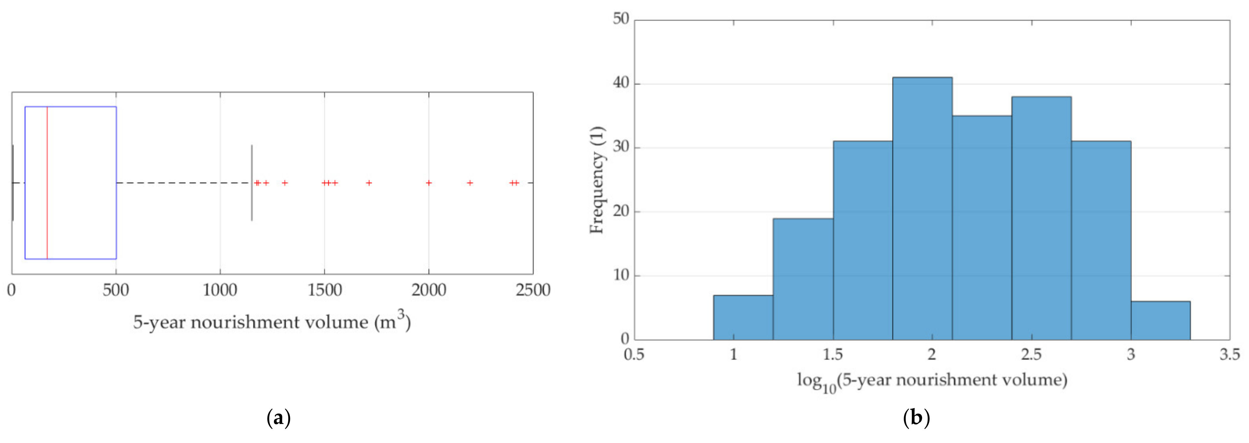
3.1. Beach Nourishment Data

Figure 1a shows a box plot of the surveyed 5-year gravel nourishment volumes along the Croatian coast, with 20 outliers marked with crosses. Here, outliers are defined when they are 1.5 interquartile ranges (IQRs) above the 75th quantile as the data is not normally distributed. Outliers account for the top 8.7% of the dataset. These outliers were not included into ANN. As shown in Figure 1a, the data is too sparse in the region above 1150 m³ to train a reliable ANN. The distribution is extremely right-skewed, as expected when 0 m³ acts as a natural boundary for the dataset because beach nourishment volume cannot have a negative value. Nourishment volumes are always positive values. A log transformation function is commonly applied to highly skewed distribution types. After the log transformation, the 5-year nourishment volume distribution takes a shape similar to a normal distribution, but still negatively skewed (Figure 1b).

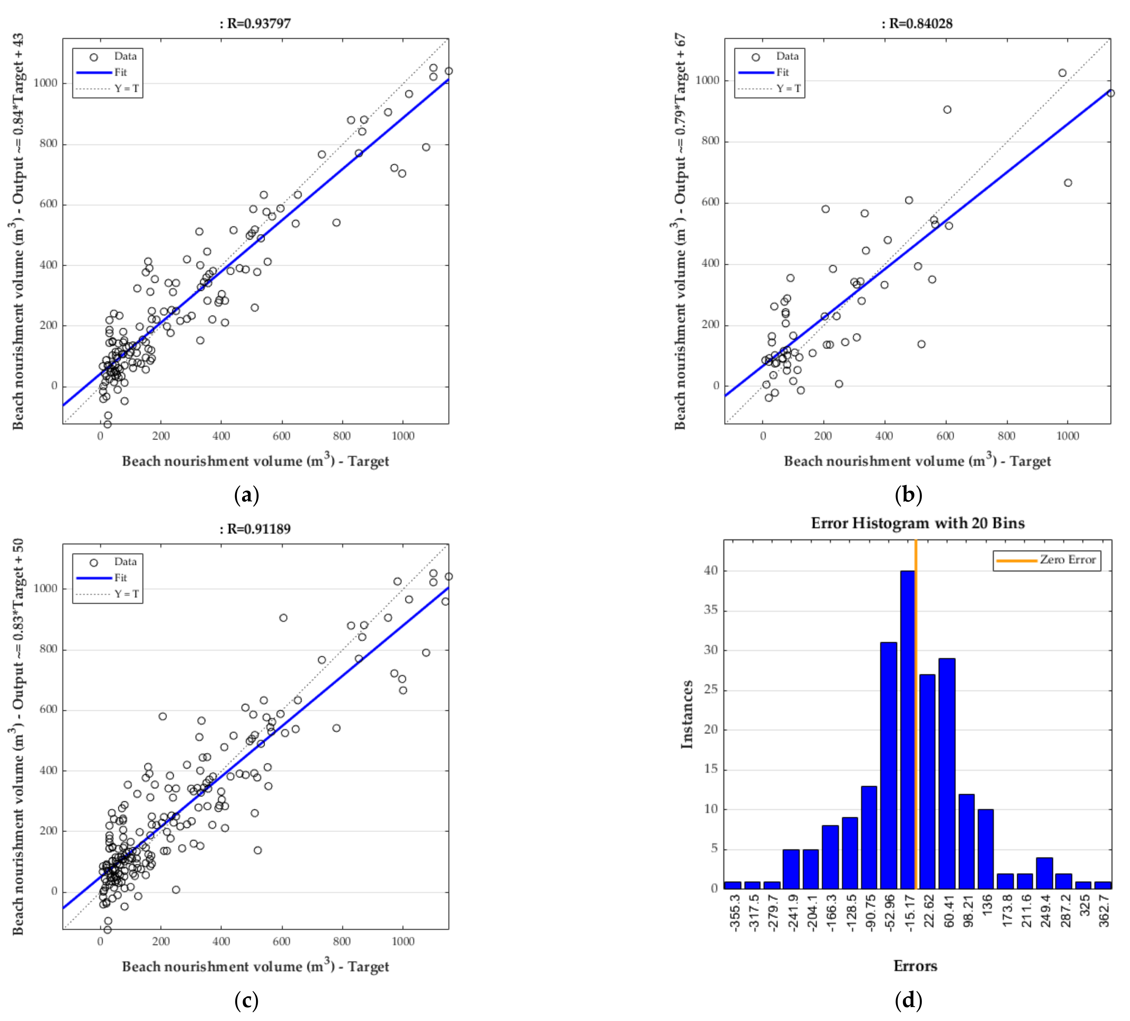
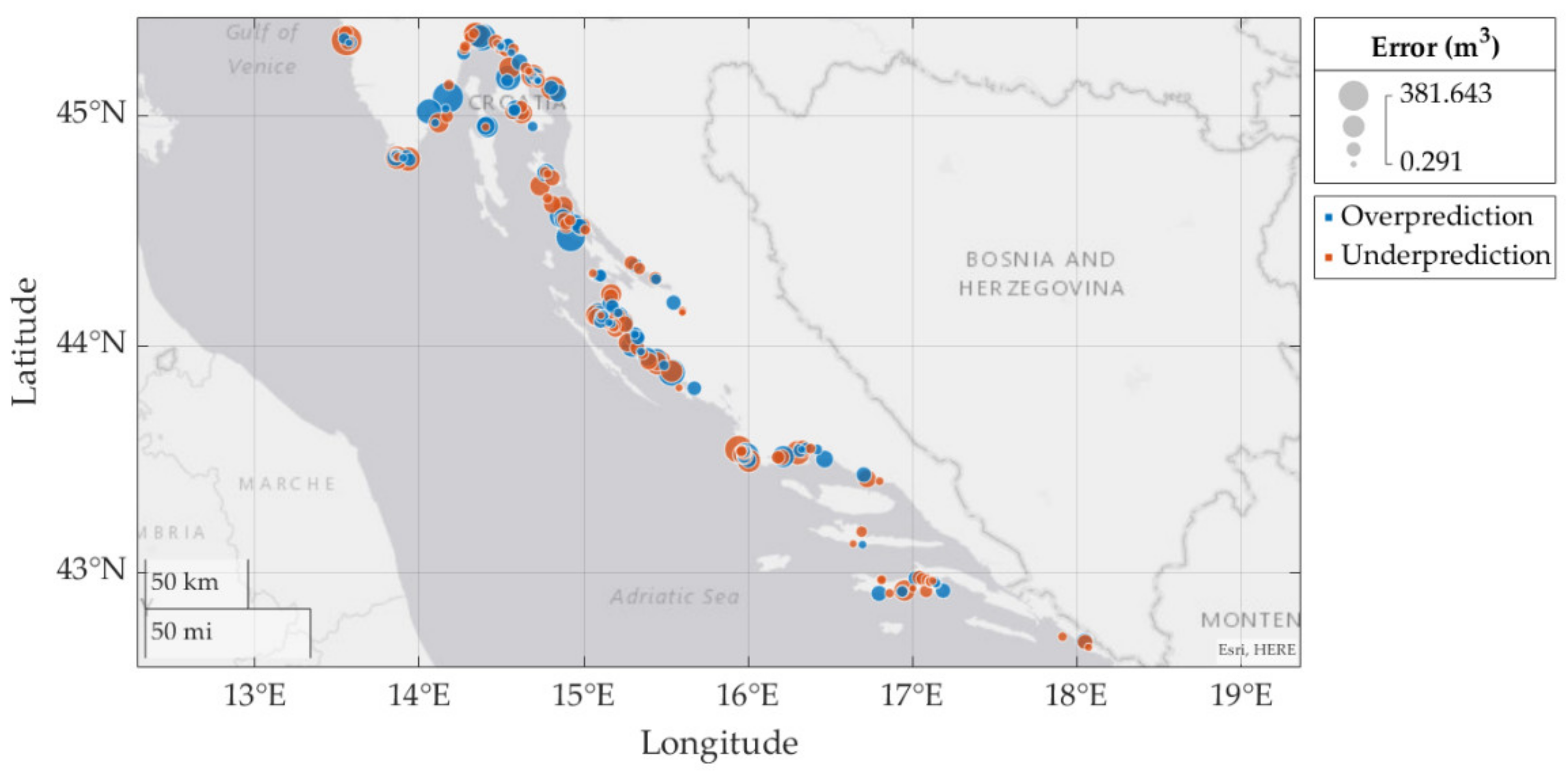
3.2. Artifical Neural Network Model Results

An ANN trained and tested using all 15 input data variables (All network) presented in Table 1 shows good prediction ability for beach nourishment volumes (Figure 2a–c). Mean squared errors are 9.63 × 10³, 1.96 × 10⁴, and 1.26 × 10⁴, for the training set, test set, and overall set, respectively. The corresponding RMSE are 98.13 m³, 140 m³, and 112.25 m³, for the training set, test set, and overall set, respectively. When normalized with the beach nourishment data range, values of 8.53%, 12.17%, and 9.76% are obtained for the training set, test set, and overall set, respectively. These NRMSEs are acceptable because they are at about 10% of the beach nourishment range. Correlation coefficients between the target (observed) and output (predicted) data for the training, test, and overall (training and test) show a strong positive relationship. Correlation coefficients are 0.94, 0.84, and 0.91 for the training set, test set, and overall set, respectively. However, the ANN underestimates the observed values as the beach nourishment volume (target value) increases, which is shown by the regression slope being below 1. The error histogram for the overall set is normally distributed (Figure 2d). This means that there are no inherent biases when the regression equation is applied. The standard deviation of the error histogram equals 76.9 m³. For an average beach area of 6834.01 (

Table 2. Expected beach characteristic based upon means for observed values for each characteristic.

Number	Data	Min	Mean	Max	Dimension
1	Beach length	12	370	2000	meters
2	Beach area	32	6834.01	104,020	square meters
3	Beach orientation (azimuth)	0	192.69	359	degrees
4	Gravel diameter	1	14.82	32	millimeters
5	Fetch length in NE direction	0.54	1033.98	19,259	meters
6	Fetch length in SE direction	0.85	4663.27	108,701	meters
7	Fetch length in SW direction	0.79	11,422.14	137,514	meters
8	Mean yearly number of days when the wind is stronger than 6 Bf	12.90	48.84	123.90	days
9	Mean yearly number of days when the wind is stronger than 8 Bf	0.6	9.10	33.30	days
10	Mean tide range	0.23	0.30	0.48	meters
11	Mean extreme tide range	0.29	0.42	0.67	meters

) this is equal to about 0.01 m in height. There is a 95% probability that the target value will be within the range of output ± 153.8 m³. This could serve to the network user as a model uncertainty indication.

As shown in Figure 2a,b, the data spread is higher for the test set in comparison to the training set as to expect. This is reflected in a higher mean squared error for the test set than the training set. Still, the correlation coefficient shows a strong relationship between the output and target values. This shows ANN’s good ability to generalize the model to unseen data. The ANN underperforms in predicting values near 0 m³ as it sometimes predicts negative values, which is unreasonable. The ANNs with different hidden layer sizes (5, 7, 10, 12, 15, and 20 neurons) revealed no significant variation in network performance on the test set (not shown in this paper). For the rest of the modelling, only networks with 15 neurons in the hidden layer were trained.

The ANN does not overpredict or underpredict certain geographic regions (Figure 3). Overprediction and underprediction of the ANN are evenly spread throughout the Croatian coast. This shows that the ANN is not sensitive to region specifics like geology, geomorphology and meteorology. However, the error values for prediction of nourishment values in the Croatia’s southern part (below 43.5° N) tend to be smaller than the rest. The mean absolute error for Croatia’s southern part equals 49.41 m³, and 88.23 m³ for the rest of Croatia’s coast. The mean absolute error for the whole coast equals 81.96 m³. As a result, the ANN should not massively overpredict or underpredict the gravel nourishment volumes of a certain region for an unseen test case.

3.3. Evaluation of Input Variable Groups Contribution to ANN Prediction Skill

In the present study, we compared ANN’s predictive ability for different input groups as shown in Table 1—column 4 and described in Section 2. Only the test set performance metric (mean squared error according to Equation (3) was considered when comparing ANNs (Figure 3). This way the network’s generalization skill to unseen data is considered.

Firstly, the check network is considered. The check network is normally expected to have perfect performance scores as it includes the target itself. This serves to test the network solving technique. As shown in Figure 4, the check network does indeed have a perfect performance score with virtually no error and perfect correlation.

Further, the ANN trained only with the input of basic group variables showed low prediction skill (Figure 4). The basic group consisted of beach length, area, azimuth, longitude and latitude. The correlation coefficient and mean square error for the test set were equal to 0.47 and 5.96 × 10⁴, respectively. Thus, using only easily extracted map data, the network has low prediction ability.

When ANN’s input comprised the basic and one other variable group, the best results were obtained by adding the fetch variable group (Figure 4). The correlation coefficient and mean square error for the test set were equal to 0.77 and 2.85 × 10⁴, respectively. Hence, including the basic map information together with fetch data gives a good prediction of gravel volume requirements. Gravel, wind, and tide group variables when added to the basic group variables moderately improved network prediction ability and will be considered further in the Combined group set (Figure 4). Rainfall contributed to some extent, but the network’s mean square error was high at 5.24 × 10⁴ on the test set. The rainfall was taken into account as many Croatian beaches are affected by torrential surface flows. However, rainfall has a limited effect on beach nourishment volume prediction. Therefore, rainfall was not considered further.

Interestingly, it was observed from the comparative analysis that the inclusion of beach slope did not add value to ANN prediction ability (Figure 4). The performance metrics with and without the inclusion of the beach slope remained the same. There might be various reasons for this lack of significance. These will be discussed further in Section 4.

A combined group variable was formed to train an ANN to match the performance of the ANN with the All group variable (includes all 15 variables and presented in Section 3.2). The input for the combined group variable comprised the basic, gravel, fetch, wind, tide group variables. The correlation coefficient and mean square error for the test set were equal to 0.83 and 2.23 × 10⁴, respectively.

The mean square error is 13.8% higher than for the All group variable, and the correlation coefficient decreases by 1%. When beach location coordinates were left out from the Combined group variable, no clear decrease in ANN prediction ability is evident. Knowledge already contributed by other included variable groups included might make the beach coordinates irrelevant. For example, latitude would be important only if a northern region has a pattern of bigger or smaller gravel nourishment volume requirements in comparison to the south. In that case, the ANN would include the location knowledge into the nourishment volume prediction with beach coordinates. To sum up, the Combined group variable without beach coordinates (Combined—Coord) is declared the best ANN because of its decreased number of required input variables without losing prediction ability of beach nourishment volumes.

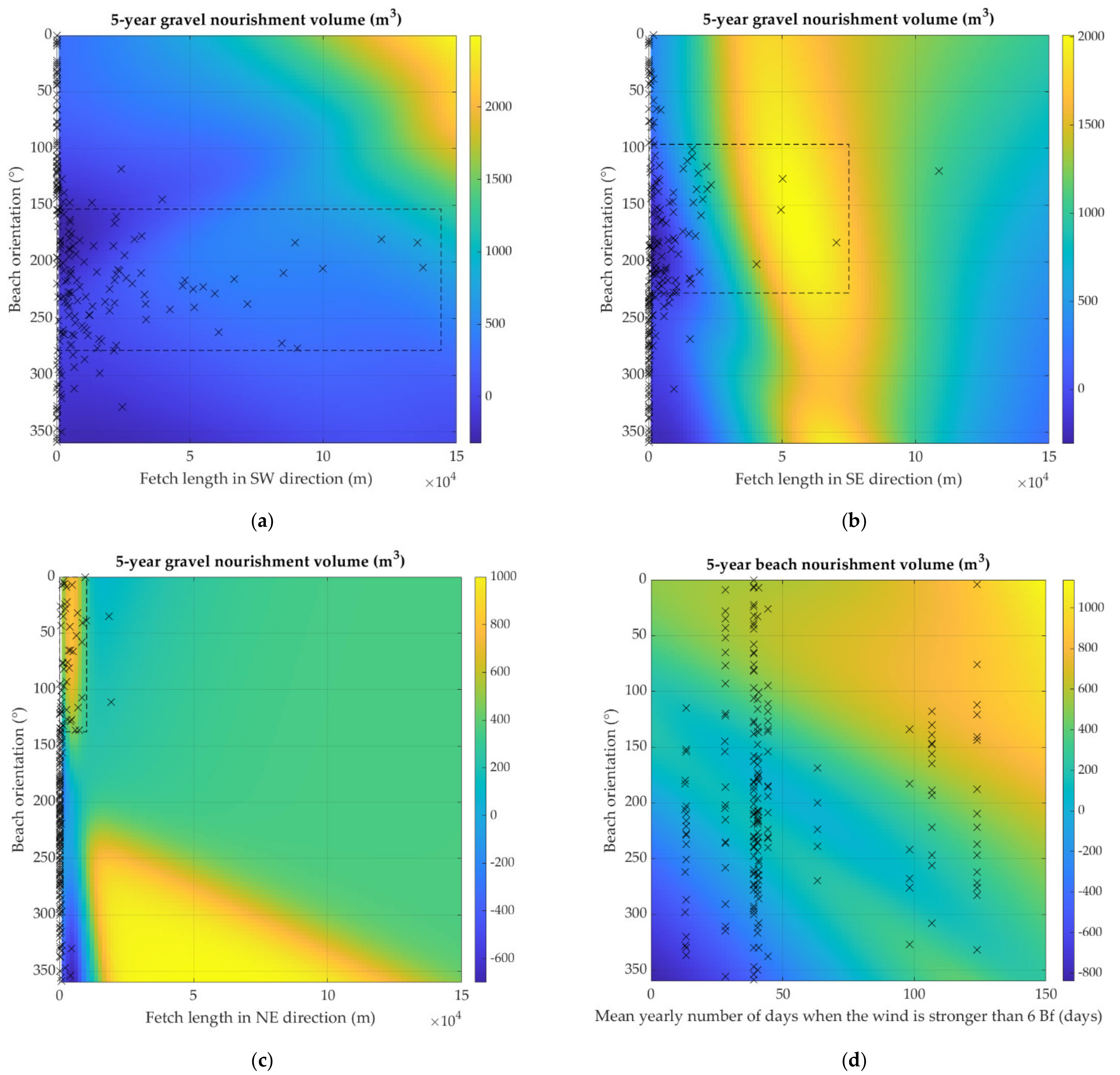
3.4. Sensitivity Analysis of the ANN to Beach Orientation, Fetch, and Wind Variables

To analyze the sensitivity of the ANN, we changed the values of one variable at time, while keeping the other variables constant. For latter we used mean observed values in Croatia (Table 2). Additionally, when one fetch length is varied to examine the ANN’s response, the other two are fixed to zero. Also, when the mean yearly number of days with wind stronger than 6 Bf is varied, the mean yearly number of days with wind stronger than 8 Bf was fixed at 5 times smaller than the one used for duration of wind above 6 Bf. This sensitivity analysis was conducted on the Combined model without coordinates (Combined—Coord) (Figure 4), which showed performance similar to the All ANN.

Figure 5 reveals an extremely nonlinear response of the ANN to the reconstructed test cases. Predictions that extend far beyond the value range considered in the training dataset can lead to unphysical results. Therefore, with a black dashed box, we have designated the region where the data should be reliable. For instance, the 5-year gravel nourishment volumes decrease if the fetch length in the SE direction increases above 8 km (Figure 5b). However, this might not be a reliable prediction because there is only one data point beyond the designated region. Thus, the black boxes are regions where the ANN calculates an interpolation of the training data.

It should be noted that the ANN can also carry out calculations even for unrealistic inputs. For example, if we assume a beach orientation in the SW direction (225 degrees), the NE fetch length should physically be close to zero (black crosses in Figure 5c). However, any other fetch length can be inputted into the network and ANN will always produce an output as one can see in Figure 5c. However, this could be unphysical. In contrary the reliable regions for SW and SE fetch lengths are much larger. And in the case of mean yearly number of days when the wind is stronger than 6 Bf, the whole domain is considered reliable because the training data spans the entire area (Figure 5d).

Figure 5a–c reveals that an increase in the fetch length in any direction increases the 5-year gravel nourishment volumes which is expected (in the reliable region designated with the black box). A fetch length increase in the NE direction shows the biggest increase in 5-year gravel nourishment volumes at 0.09 m³ per meter of fetch length. The increase is 3 times lower for the SE direction at 0.03 m³ per meter of fetch length, and 30 times lower for the SW direction at 0.003 m³ per meter of fetch length. These results show significant susceptibility of 5-year gravel nourishment volumes to the wind and waves from the NE direction. For the most part of Croatia’s coast, the NE wind tends to be a seaward wind. This is not the case for island beaches and some other, where a NE direction orientation is likely.

Figure 5d shows that an increase in mean yearly number of days when the wind is stronger than 6 Bf results in an increase of the 5-year nourishment volumes. This is an expected behavior, because it is assumed that an increase in windy days will increase the number of days with waves. When the beach is exposed to NE waves, the ANN tends to output the highest values of 5-year gravel nourishment volume. Again, pointing to the NE wind as having the most erosion potential of the 3 considered wind directions (NE, SE, and SW). On the other hand, the beach orientation toward the NW tends to have the lowest values. The Figure 5d shows also the ANN ambiguity with beach orientation of 0 and 360 degrees, which are considered as two different orientations.

4. Discussion

This study has shown that the ANN and observation data can be used to adequately predict the observed spatial variability of gravel nourishment volumes on Croatian beaches. The significance of the obtained results and in particular the importance of different variables for the prediction of beach nourishment volumes are discussed in the context of other studies, as there are no other ANN models to compare the results with.

Tides were found to have a moderate influence on ANN accuracy (Figure 4). This contrasts with the findings of Yates and Le Cozannet [22], that tidal range and wave height had a similar influence on the network prediction ability. This is not surprising, however, as there is more variation in tidal ranges across the entire European continent than on the Croatian coast. The eastern Adriatic Sea has a microtidal regime with tidal ranges of less than 2 m and with very little regional variation.

Waves (indirectly via the fetch length) had a significantly greater influence on the predictive ability of the ANN. The fetch length turned out to be a more important variable than the annual mean number of windy days. Another study by Wilson, Adams [3] reported that wave runup had a bigger influence on network prediction ability than WIH alone (wave impact hours). We indirectly confirmed this in this paper, as the fetch length had a more important impact than the yearly mean number of windy days.

The beach slope was expected to be an important factor in beach nourishment modelling, as the beach slope influences the transformation of the nearshore waves, and hence the driving forces behind beach changes as well as the beach stability. However, this variable was not selected by the ANN. One possible explanation for this is that beach slopes were extracted from navigational maps that are not detailed enough near the coastline to provide reliable slope data. On the other hand, beach slope is difficult to integrate into the ANN model because it is a time-dependent variable. Beach slopes are often stepper after winter wave storms that greatly reshape beach profiles and often generate onshore berms. By comparison, the beach slope is flatter after the summer tourist season and a milder wave climate. Anthropogenic influences like gravel nourishment can also alter the beach slope in the nearshore. Wilson et al. [3] established an event-based network where the beach slopes could be updated after every event, but this could not be implemented into our ANN model.

The gravel diameter was found to be an important variable for the ANN predictions. This is in agreement with the findings of previous studies that the gravel diameter primarily dictates the equilibrium beach profile generated by cross-shore sediment processes [8,9]. Also, the beach slope is dependent on the gravel diameter and this may be why the gravel size information influenced the ANN’s prediction ability more than the beach slope itself.

However, the developed ANN has some limitations. Section 3.4 highlights how even unphysical and unrealistic input variables could be fed to the ANN resulting in an unreliable output. Users should always remember not to use input variables that differ greatly from the parameter space over which the ANN has been established because the predictions could be unphysical and unreliable. This was often highlighted in previous research [7,14]. The ANN is not fitted with a procedure to determine if the input data is reasonable or even physically sound. This could be handled only with a preprocessing procedure created for the ANN’s specific use case. This preprocessing procedure can limit extrapolation of the training dataset and non-physical input combinations.

This is a disadvantage of the ANN model compared to the Bayesian network models. Bayesian networks use predefined bins for each category (e.g., beach nourishment volume) to conduct probabilistic predictions [3,22]. Predefined bins can easily limit the input data that is out of the trained parameter space or deemed unphysical. The approach handles probabilities directly in contrast to the ANN, which estimates a specific value. Moreover, this approach implicitly gives model uncertainties for each output. This uncertainty information could be valuable to the user when applying the model to unseen test data sets. This advantage of the Bayesian networks can also be a disadvantage if a specific value is required and not just the highest probability category bin. For example, Yates and Le Cozannet [22] used Bayesian networks to predict if a coastline is accreting, stable, or eroding. They did not include information on the amount of erosion and did not focus on gravel or sand beaches. The simple yes/no erosion information is probably not sufficient for operational coastal management on a local level, e.g., beach nourishment volumes. Thus, despite limitations, the ANN could be useful for forecasting beach replenishment volumes and thus for operational coastal management.

5. Conclusions

The results of this study show that an ANN can adequately predict the observed gravel nourishment volume spatial variability on Croatian beaches on unseen data. Tests revealed a strong correlation between the observations and the ANN’s output. The correlation coefficient and mean square error for the test set equal 0.87 and 2.24 × 10⁴, respectively (Combined—coords group variable which includes beach area, beach length, beach orientation, fetch length, gravel size, mean yearly number of days when the wind is stronger 6 Bf and 8 Bf, and tide range). Other tested variables like beach slope, location coordinates, and rainfall had little or no contribution to the ANN’s prediction ability.

The results show that fetch length was found to be the most important input variable, apart from the basic information derived from maps such as beach length, beach area and beach orientation for ANN’s prediction ability. The fetch length and beach orientation are parameters that determine the height and direction of the wind wave and are therefore proxies for forcing. Fetch length in the NE direction showed the greatest impact on the gravel nourishment requirements; three times stronger impact than fetch length in the SE and 30 times stronger than fetch length in the SW direction. Beach orientation also points to the NE direction as the most impactful to beach nourishment volume requirements. Since the training set was limited to Croatian coast, further data in other countries is needed to expand this ANN gravel prediction model.

References

1. Hinrichsen, D. The Coastal Population Explosion. The Next 25 Years: Global Issues. In Trends and Future Challenges for US National Ocean and Coastal Policy: Proceedings of a Workshop; NOAA: Washington, DC, USA, 1998; pp. 27–29. [Google Scholar]
2. Pikelj, K.; Ruzic, I.; Ilic, S.; James, M.R.; Kordic, B. Implementing an efficient beach erosion monitoring system for coastal management in Croatia. Ocean Coast. Manag. 2018, 156, 223–238. [Google Scholar] [CrossRef] [Green Version]
3. Wilson, K.E.; Adams, P.N.; Hapke, C.J.; Lentz, E.E.; Brenner, O. Application of Bayesian Networks to hindcast barrier island morphodynamics. Coast. Eng. 2015, 102, 30–43. [Google Scholar] [CrossRef]
4. Bogaert, P.; Montreuil, A.-L.; Chen, M. Predicting Morphodynamics for Beach Intertidal Systems in the North Sea: A Space-Time Stochastic Approach. J. Mar. Sci. Eng. 2020, 8, 901. [Google Scholar] [CrossRef]
5. Gunawardena, Y.; Ilic, S.; Pinkerton, H.; Romanowicz, R. Nonlinear transfer function modelling of beach morphology at Duck, North Carolina. Coast. Eng. 2009, 56, 46–58. [Google Scholar] [CrossRef] [Green Version]
6. Southgate, H.N. Data-based yearly forecasting of beach volumes along the Dutch North Sea coast. Coast. Eng. 2011, 58, 749–760. [Google Scholar] [CrossRef]
7. Goldstein, E.B.; Coco, G.; Plant, N.G. A review of machine learning applications to coastal sediment transport and morphodynamics. Earth Sci. Rev. 2019, 194, 97–108. [Google Scholar] [CrossRef] [Green Version]
8. U.S. Army Corps of Engineers (USACE). Coastal Engineering Manual; USACE: Washington, DC, USA, 2008; p. 477.
9. Dean, R.G. Coastal Sediment Processes: Toward Engineering Solutions. In Proceedings of Coastal Sediments’87, Specialty Conference on Advances in Understanding of Coastal Sediment Processes, New Orleans, LA, USA, 12–13 May 1987; pp. 1–24. [Google Scholar]
10. Van Wellen, E.; Chadwick, A.J.; Mason, T. A review and assessment of longshore sediment transport equations for coarse-grained beaches. Coast. Eng. 2000, 40, 243–275. [Google Scholar] [CrossRef]
11. van Rijn, L.C. A simple general expression for longshore transport of sand, gravel and shingle. Coast. Eng. 2014, 90, 23–39. [Google Scholar] [CrossRef]
12. Hanson, H. Genesis—A Generalized Shoreline Change Numerical-Model. J. Coast. Res. 1989, 5, 1–27. [Google Scholar]
13. Tomasicchio, G.R.; Francone, A.; Simmonds, D.J.; D’Alessandro, F.; Frega, F. Prediction of Shoreline Evolution. Reliability of a General Model for the Mixed Beach Case. J. Mar. Sci. Eng. 2020, 8, 361. [Google Scholar]
14. van Maanen, B.; Coco, G.; Bryan, K.R.; Ruessink, B.G. The use of artificial neural networks to analyze and predict alongshore sediment transport. Nonlinear Process. Geophys. 2010, 17, 395–404. [Google Scholar] [CrossRef]
15. Brunton, S.L.; Noack, B.R.; Koumoutsakos, P. Machine Learning for Fluid Mechanics. Annu. Rev. Fluid Mech. 2020, 52, 477–508. [Google Scholar] [CrossRef] [Green Version]
16. Olden, J.D.; Joy, M.K.; Death, R.G. An accurate comparison of methods for quantifying variable importance in artificial neural networks using simulated data. Ecol. Model. 2004, 178, 389–397. [Google Scholar] [CrossRef]
17. Plant, N.G.; Stockdon, H.F. Probabilistic prediction of barrier-island response to hurricanes. J. Geophys. Res. Earth Surf. 2012, 117. [Google Scholar] [CrossRef]
18. Hashemi, M.R.; Ghadampour, Z.; Neill, S.P. Using an artificial neural network to model seasonal changes in beach profiles. Ocean Eng. 2010, 37, 1345–1356. [Google Scholar] [CrossRef]
19. Tsekouras, G.E.; Rigos, A.; Chatzipavlis, A.; Velegrakis, A. A Neural-Fuzzy Network Based on Hermite Polynomials to Predict the Coastal Erosion. In Engineering Applications of Neural Networks; Springer: Cham, Switzerland, 2015; pp. 195–205. [Google Scholar] [CrossRef]
20. Rigos, A.; Tsekouras, G.E.; Chatzipavlis, A.; Velegrakis, A.F. Modeling Beach Rotation Using a Novel Legendre Polynomial Feedforward Neural Network Trained by Nonlinear Constrained Optimization. In Artificial Intelligence Applications and Innovations; Springer: Cham, Switzerland, 2016; pp. 167–179. [Google Scholar] [CrossRef] [Green Version]
21. Iglesias, G.; Lopez, I.; Castro, A.; Carballo, R. Neural network modelling of planform geometry of headland-bay beaches. Geomorphology 2009, 103, 577–587. [Google Scholar] [CrossRef]
22. Yates, M.L.; Le Cozannet, G. Brief communication ‘Evaluating European Coastal Evolution using Bayesian Networks’. Nat. Hazards Earth Syst. Sci. 2012, 12, 1173–1177. [Google Scholar] [CrossRef]
23. Lentz, E.E.; Hapke, C.J. Geologic framework influences on the geomorphology of an anthropogenically modified barrier island: Assessment of dune/beach changes at Fire Island, New York. Geomorphology 2011, 126, 82–96. [Google Scholar] [CrossRef]
24. Hrvatski Hidrografski Institut (HHI). Peljar za Male Brodove—Drugi dio: Sedmovraće—Rt. Oštra; HHI: Split, Croatia, 2020; p. 312. [Google Scholar]
25. Mackay, D.J.C. Bayesian Interpolation. Neural Comput. 1992, 4, 415–447. [Google Scholar] [CrossRef]
26. Faraway, J.; Chatfield, C. Time series forecasting with neural networks: A comparative study using the airline data. J. R. Stat. Soc. Ser. C Appl. Stat. 1998, 47, 231–250. [Google Scholar] [CrossRef]
27. Kolen, J.F.; Pollack, J.B. Back Propagation is Sensitive to Initial Conditions. In Proceedings of the 3rd International Conference on Neural Information Processing Systems, Denver, CO, USA, 26 November 1990; pp. 860–867. [Google Scholar]
Figure 1. Distribution of 5-year gravel nourishment volumes that have been reported by counties in the survey: (a) box plot with specified outliers; (b) log transformed 5-year nourishment volumes correspond to a normal distribution.
Jmse 09 00786 g001
Figure 2. Correlation and scatter plot for the target (observed) and output (predicted using ANN) data: (a) training set; (b) test set; (c) overall (training and test set); (d) error histogram for the overall data set (training and test set) in (c).
Jmse 09 00786 g002
Figure 3. Mapped errors (target and output value differences) with underprediction and overprediction presented in orange and blue respectively; the bubble size indicates error size.
Jmse 09 00786 g003
Figure 4. Performance statistics for tested ANNs on the test data sets according to equation 3—bar chart of mean squared errors (lower is better) on the left y-axis; stem chart of correlation coefficients (higher is better) on the right y-axis; variables included in each group can be found in Table 1; Combined group comprises Basic + Gravel + Fetch + Wind + Tide; training set, test set, and overall (training and test set) performance statistics are presented in Table A1, Appendix A.
Jmse 09 00786 g004
Figure 5. Sensitivity analysis presented with a heat map of the best-performing ANN (combined group variables without the beach coordinates) and scatter plot of available data (black crosses): (a) fetch length in the SW direction—beach orientation; (b) fetch length in the SE direction—beach orientation; (c) fetch length in the NE direction—beach orientation; (d) Mean yearly number of days when the wind is stronger than 6 Bf—beach orientation; the dashed black box designates the area where predictions are considered reliable because the ANN calculates an interpolation of the training data.
Jmse 09 00786 g005