
Relationship between Three-Dimensional Radiation Stress and Vortex-Force Representations


1
Department of Coastal & Urban Risk & Resilience, IHE Delft Institute for Water Education, 2611 AX Delft, The Netherlands
2
Faculty of Civil Engineering and Geosciences, Delft University of Technology, 2628 CN Delft, The Netherlands
3
Vietnam Institute of Seas and Islands, Hanoi 113000, Vietnam
4
Deltares, 2629 HV Delft, The Netherlands
*
Author to whom correspondence should be addressed.
J. Mar. Sci. Eng. 2021, 9(8), 791; https://0-doi-org.brum.beds.ac.uk/10.3390/jmse9080791
Submission received: 31 May 2021
/
Revised: 18 July 2021
/
Accepted: 20 July 2021
/
Published: 22 July 2021
(This article belongs to the Section Ocean Engineering)
Abstract
:In numerical ocean models, the effect of waves on currents is usually expressed by either vortex-force or radiation stress representations. In this paper, the differences and similarities between those two representations are investigated in detail in conditions of both conservative and nonconservative waves. In addition, comparisons between different sets of equations of mean motion that apply different representations of wave-induced forcing terms are included. The comparisons are useful for selecting a suitable numerical ocean model to simulate the mean current in conditions of waves combined with currents.
1. Introduction
In literature, wave-induced momentum flux is expressed in terms of either ‘radiation stress’ or ‘vortex force’ representations. Both representations have been applied widely in ocean and coastal numerical models.
The radiation stress representation was introduced by Longuet-Higgins and Stewart [1]. It was successful in explaining the transfer of momentum flux from the waves to the mean current. However, it is a two-dimensional (2D) tensor, and as such it is only suitable for depth-averaged numerical models. The extension of the ‘traditional’ radiation stress concept to three-dimensional (3D) space has been the subject of many studies. In Xia, Xia [2], the 3D radiation stress was inferred from the classical 2D radiation stress concept of Longuet-Higgins and Stewart [1]. This method was also applied by Mellor [3]. However, as indicated by Ardhuin, Suzuki [4], this method is “incorrect because of a derivation error”. Recently, Nguyen, Jacobsen [5] obtained a depth-dependent wave radiation stress tensor in the Generalized Lagrangian Mean (GLM) framework. It was applied in their quasi-Eulerian mean equations of motion. With the use of the depth-dependent wave radiation stress formulation, their equations were successfully validated with various experimental data in conditions of waves combined with currents.
The vortex force representation is an alternative way to express the mean effect of waves on the current. It was first introduced by Craik and Leibovich [6] to explain the evolution of Langmuir circulations. The vortex-force representation involves a gradient of the Bernoulli head and a vortex force. This concept has been widely applied by the ocean and coastal communities such as McWilliams, Restrepo [7], Newberger and Allen [8], Ardhuin, Rascle [9] Michaud, Marsaleix [10]; and Bennis, Ardhuin [11].
In Lane, Restrepo [12], a comparison of ‘radiation stress’ and ‘vortex force’ representations was made. Their study showed that these two representations are equivalent for conservative waves. However, the relationship between these two representations for non-conservative waves was not addressed in their study.
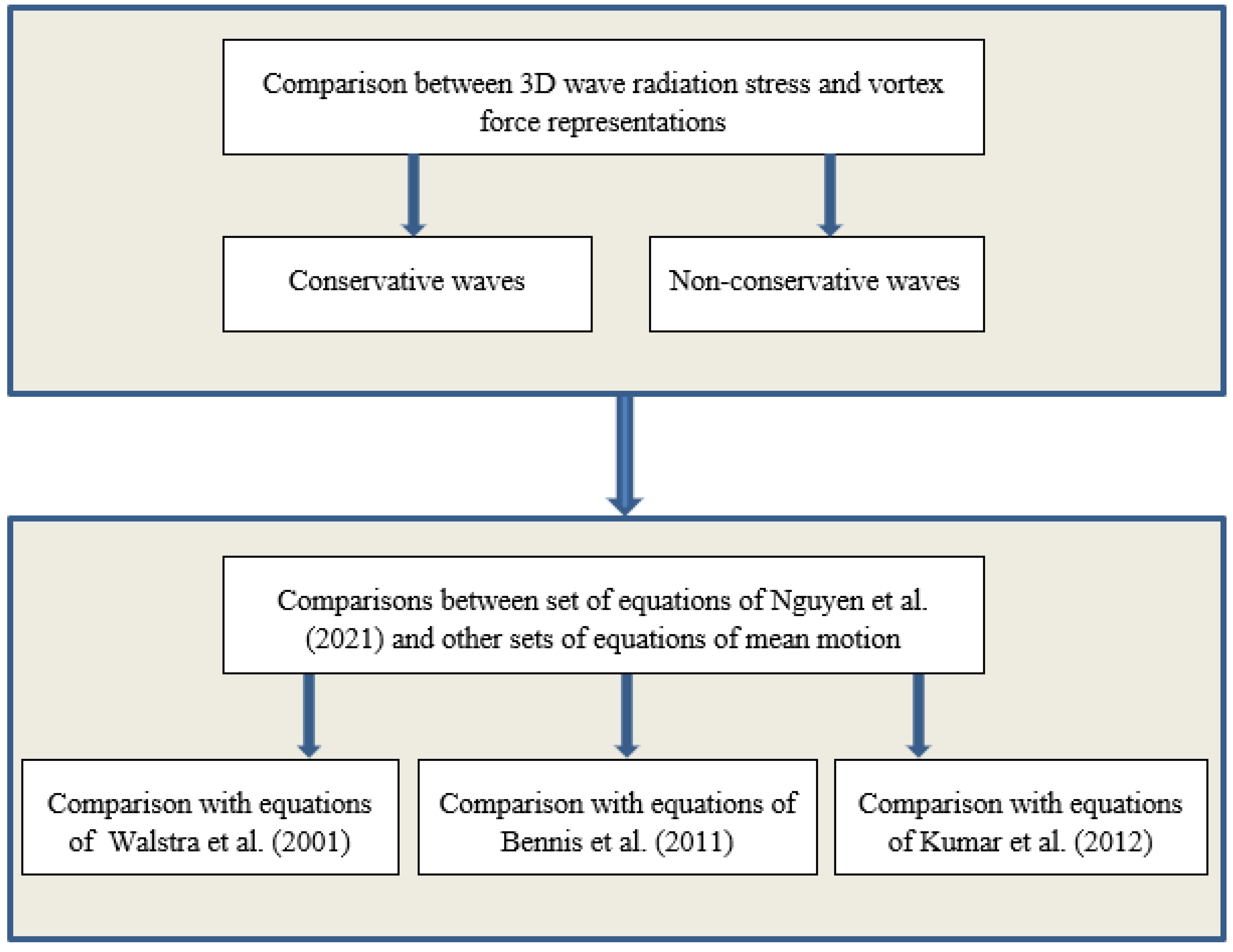
This present work thus aims at studying the relationship between three-dimensional wave radiation stress, introduced by Nguyen, Jacobsen [5], and vortex-force representations in both conditions of conservative waves and non-conservative waves. Moreover, comparisons of several other sets of equations for the mean motion using different representations of wave-induced forcing terms are given. This can be useful in choosing a suitable numerical model to simulate the mean current in different conditions of waves combined with mean currents. A flowchart that describes the methodology of this study is presented in Figure 1.
2. Radiation Stress and Vortex Force Representations
2.1. Three-Dimensional Wave Radiation Stress Representation
The components of three-dimensional wave radiation stress tensor S are defined by:
where, is the wave velocity, and is water density. If the surface wave amplitude is slowly modulating then local linear wave theory can be applied to calculate the horizontal wave radiation stress components. In the presence of dissipative forcing and a strong current, the vertical components of wave radiation stress change very fast with depth. To account for this the vertical components of wave radiation stress are decomposed as [5]:
where the subscript CS presents the conservative part of the vertical component of wave radiation stress, is wave-induced forcing caused by breaking waves and rollers, and is wave-induced mixing. The vertical distributions of and can be estimated with empirical formulas given by Uchiyama, McWilliams [13]. Using local linear wave theory the horizontal components of wave radiation stress can be calculated, resulting in the radiation stress forcing:
where, is the Stokes drift and the effect of Coriolis on the wave-induced current is added with as Coriolis frequency, Ω the angular velocity of the Earth, and the latitude at the given position.
2.2. Vortex-Force Representation
Another way to express the effect of waves on currents is using vortex-force representation. This method was proposed by McWilliams, Restrepo [7]. In their work, the surface waves are assumed slow varying, weakly nonlinear, and irrotational up to second-order of the wave amplitude. Further, the mean currents are assumed to vary slowly and are small in comparison with the wave velocity, i.e., .
In vortex force representation, the wave-induced forcing is given by:
where, is wave-induced forcing in terms of vortex force representation, is the quasi-Eulerian mean velocity, and is wave-induced kinematic pressure defined by:
where, is the wave amplitude, is the wavenumber, is the gravitational acceleration of the Earth, and is the still water depth.
2.3. Relationship between Wave Radiation Stress and Vortex Force Representations
2.3.1. General Formulation
Both wave radiation stress and vortex-force representations are applied widely in the ocean and coastal numerical models. In this section, the relationship between those two representations is presented using the GLM method proposed by Andrews and McIntyre [14].
For any quantity , the following notation is employed:
where, is the disturbance displacement of a fluid particle.
We start with the momentum equation for total flow in the ith-direction (i runs from 1 to 3) evaluated at disturbance position of fluid-particle [5]:
where, , is pressure, and is a non-wave forcing term. The Kronecker delta function is defined by:
In the following, the gravitational acceleration g is assumed a constant, and the non-wave forcing term is neglected. Multiplying Equation (14) with and averaging over wave period the following equation for the evolution of Lagrangian disturbance velocity is obtained:
where the Einstein summation convention is applied with j running from 1 to 3, is the Lagrangian mean material derivative, is the GLM velocity, the nabla operator, and is the Lagrangian disturbance of any mean quantity [14].
Next, we consider the pseudo-momentum defined by [14]:
Using the relation [14] and definition (17), the first term on the left-hand side of the Equation (16) can be expressed as:
where, the Einstein summation convention is applied to j and k (j and k run from 1 to 3).
The second term on the left-hand side of the Equation (16) is approximated by:
For the third term on the left-hand side of the Equation (16) we make use of the fact that for any quantity the relationship between Lagrangian disturbance and quasi-Eulerian disturbance is given by [14]:
where, is a small parameter, and is the quasi-Eulerian disturbance of quantity . Ignoring the effects of turbulence, the quasi-Eulerian disturbance is replaced by wave quantity . Then, the third term on the left-hand side of the Equation (16) can be expressed by:
where, is the Stokes correction of mean pressure.
From Equations (18), (19), and (21), the Equation (16) is rewritten as:
According to Nguyen, Jacobsen [5] (Equation (A38)), the radiation stress gradient in the ith-direction can be expressed by:
From Equations (22) and (23) we thus obtain the following equation:
Equation (24) expresses the general relationship between wave radiation stress and the vortex-force representations. In this, the first term on the right-hand side represents the changes in the wave-related Bernoulli head, and the second term on the right-hand side of the Equation (24) expresses the vortex force of the mean current. The remaining terms on the right-hand side are a function of the mismatch between the pseudo momentum and the Stokes drift. According to Andrews and McIntyre [14], the Stokes drift is defined by:
From definitions (17) and (25) we obtain:
The first term on the right-hand side of Equation (26) expresses the effect of rotation of the wave, and the second term relates to the shear-effect of the mean current. The calculation of the first term on the right-hand side of Equation (26) requires a rotational wave theory. However, the use of rotational wave theory is still a challenge for coastal and ocean applications. In the next sections, the right-hand side of Equation (24) will be expressed explicitly under specific conditions of the waves combined with the mean currents.
2.3.2. Conservative Waves
In this part, the following assumptions are applied:
- (i)
- The waves are conservative and irrotational up to the second-order of wave amplitude.
- (ii)
- The mean currents change slowly and are small in comparison with the wave velocity, i.e., .
The above conditions were also used by McWilliams, Restrepo [7] to obtain the vortex force representation. With conditions (i) and (ii), Equation (26) becomes:
Thus, the pseudo-momentum is approximately equal to the Stokes drift . Therefore, the last two terms on the right-hand side of Equation (24) can be neglected giving:
The term is the Bernoulli head in the GLM framework. From Equation (20) we obtain:
where the term K is a correction of the Bernoulli head defined by:
Using linear wave theory we obtain:
Combining (29) and (31) gives:
where the term is defined by (12).
In ocean and coastal environments, it is usually that . Therefore, the term can be neglected in the vortex force representation. From Equations (28) and (32), and including the Coriolis effect in the radiation stress forcing consistent with Equations (6)–(8), we obtain:
Equations (33)–(35) show the relationship between radiation stress and vortex force representations for conservative waves. The right-hand side of these equations is vortex force representation obtained by McWilliams, Restrepo [7] with a correction of the Bernoulli head K. Therefore, in conditions of weakly nonlinear waves and weak ambient current, the radiation stress and vortex-force representations are equivalent.
2.3.3. Non-Conservative Waves
In this section, the relationship between radiation stress and vortex force representations will be studied under the following conditions:
- (i)
- The evolution of the waves is dominated by dissipative processes, such as breaking waves, rollers, white-capping, and bottom friction.
- (ii)
- The mean currents are slowly varying and small in comparison with the wave velocity, i.e., .
In the presence of non-conservative processes, the last two terms on the right-hand side of Equation (24) express the evolution of the rotation of the waves. In the presence of wave dissipation, we do not have any relationship between and . If the current is small in comparison with the wave velocity then its effect on the wave-induced forcing can be neglected. The evolution of the rotation of the waves is approximated by dissipative wave forcing, i.e.,:
From Equations (32) and (36), Equation (24) is now expressed as:
Equations (37)–(39) express the relationship between radiation stress and vortex force representations in the condition of non-conservative waves propagating on a weak current. This shows that the wave radiation stress gradient is the total of vortex-force and nonconservative wave forcing.
3. Equations of Motion of Nguyen et al. 2020 under the Hydrostatic Assumption
3.1. Quasi-Eulerian Mean Equations of Motion
3.1.1. Equations of Motion Using the Wave Radiation Stress Representation
In this part, the equations of motion of Nguyen, Jacobsen [5] are simplified with the hydrostatic assumption of the mean flow. This means that acceleration of mean velocity and dissipative forcing are neglected in the vertical momentum equation. This assumption is suitable for most hydrodynamic problems in deep ocean and coastal zones.
Quasi-Eulerian mean quantity is defined by:
where, is GLM quantity, and is Stokes correction of mean quantity .
According to Longuet-Higgins and Stewart [15], the hydrostatic pressure is defined by:
Then, the momentum equations for the mean motion of Nguyen, Jacobsen [5] are rewritten as:
where, is the Reynolds stress, and is molecular viscosity. Local linear wave theory is applied to calculate the conservative part of the wave radiation stress. The wave-induced forcing terms and are estimated by empirical formulas given by Uchiyama, McWilliams [13].
The normal components of wave radiation stress are calculated by:
where, and are directional vector components of peak wave number , and are empirical factors representing the effect of mean current on the wave radiation stress in x- and y-directions, respectively.
The mass conservation equation is given by [5]:
where, is the Stokes correction of the mean position of the fluid particle given by:
The depth-integrated continuity equation is [5]:
3.1.2. Equations of Motion Using the Vortex Force Representation
In this section, the equations of mean motion of Nguyen, Jacobsen [5] are expressed in terms of vortex force representation. It is noticed that the vortex force representation is only valid in the condition of weak ambient current, i.e., .
From the relationship between radiation stress and vortex force representation, Equations (37)–(39), the quasi-Eulerian mean momentum Equations (42)–(44) are rewritten as:
The mass conservation is given again by Equation (47).
3.2. Generalized Lagrangian Mean Equations of Motion
In this section, Equations (42), (43), and (49) are expressed in terms of the GLM velocity. According to Ardhuin, Rascle [9], hydrostatic pressure can be expressed by:
where, is the mean atmospheric pressure at the water surface.
Using local linear wave theory, the Stokes correction of the mean pressure is given by:
Therefore, Equations (42) and (43) are expressed in terms of GLM velocity as:
where, and are defined by:
From Equation (47) we obtain mass conservation equation in GLM framework, i.e.,:
The depth-integrated continuity equation is:
where the term can be neglected in case of stationary waves.
4. Comparisons with Other Sets of Equations for the Mean Motion
4.1. Comparison with the Set of Equations of Motion of Walstra et al. 2001
The set of equations of motion of Walstra, Roelvink [16] has been implemented in the Delft3D-Flow model. Details of the implementation are given in Hydraulics [17]. It is the simplification of the set of equations developed by Groeneweg [18]. In the following, the horizontal momentum equations of Walstra, Roelvink [16] are expressed with the addition of the Coriolis effect and gradient of atmospheric pressure, i.e.,:
where, and are wave-induced driving forces given by:
where, is Stokes correction of turbulent stress.
The depth-integrated continuity equation is:
In Table 1, a comparison between the sets of equations of Walstra, Roelvink [16] and equations of Nguyen, Jacobsen [5] expressed in the GLM framework is presented for the x-direction.
Table 1 shows that the difference between Walstra, Roelvink [16] and the equations of Nguyen, Jacobsen [5] mainly comes from the wave-induced forcing terms. It shows that the terms and are absent in the conservative wave forcing term of Walstra, Roelvink [16]. Those terms are considered in Groeneweg [18], where corresponds to the evolution of . The missing second-order of wave amplitude terms leads to an imbalance of the model and generates spurious oscillations, discussed below.
Moreover, according to Nielsen and You [19], the effect of a strong current on the normal component of wave radiation stress gradient is significant. This effect was not considered by Walstra, Roelvink [16]. In Nguyen, Jacobsen [5], the normal component of wave radiation stress is enhanced by a factor that represents the effect of current on the wave radiation stress. The factor approximates to 1 in the condition of a weak current; however, it is significant in the presence of a strong current.
In Walstra, Roelvink [16], the breaking and roller wave-induced forcing term is provided as surface stress. The breaking induced turbulence is incorporated into the turbulence model as a surface boundary condition. However, this method is only suitable under the condition of strong vertical mixing due to breaking waves [20]. In addition, the Stokes correction of turbulent stress is a term of third-order of the wave amplitude, i.e., . Therefore, it can be neglected if the equations of motion are expressed to the second-order of wave amplitude.
In Nguyen, Jacobsen [5], the breaking wave and roller wave-induced forcing term is applied as a body force. This method is suitable for both strong and weak vertical mixing conditions, where the empirical formulas proposed by Uchiyama, McWilliams [13] are applied to calculate the vertical distribution of wave breaking induced forcing term.
The mass conservation equation of Walstra, Roelvink [16] is equivalent to the mass conservation equation of Nguyen, Jacobsen [5] if the surface waves change slowly in time.
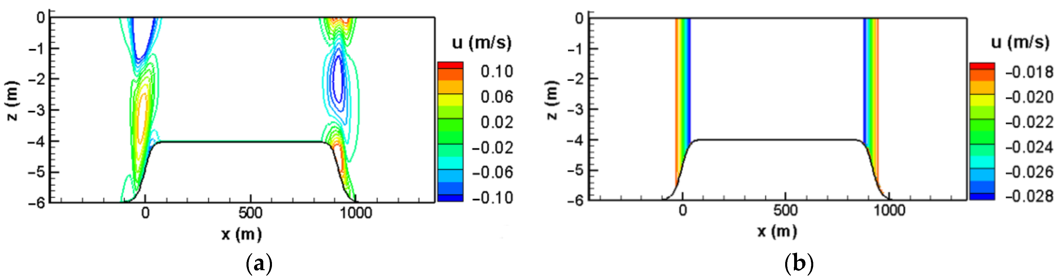
In the following, an adiabatic test proposed by Bennis, Ardhuin [11] is employed to test the equations of Walstra, Roelvink [16]. In this, a monochromatic wave propagates on a slope without dissipation. This is a simple but very challenging test since any imbalanced forces might lead to a spurious oscillation of the mean current. The horizontal mean current should be uniform in a vertical direction even if the wave propagates on a sloping bed. The equations of Nguyen, Jacobsen [5] were successful in testing with the adiabatic condition.
In adiabatic condition, momentum Equations (61) and (62) become:
The depth-integrated continuity equation is:
The spatial distribution of quasi-Eulerian mean horizontal velocity calculated by equations of Walstra, Roelvink [16] is presented in Figure 2a. That result was obtained after 30 min of simulation time. On the slope, the horizontal velocity is non-uniform in the vertical direction. Moreover, the model is unstable and the mean velocity increases to infinity in time. Thus, the equations of Walstra, Roelvink [16] do not pass the adiabatic test. The imbalance is caused by the omission of the second-order terms and . Figure 2b presents the distribution of quasi-Eulerian mean flow simulated with the equations of Nguyen, Jacobsen [5] that include these terms showing the correct depth-uniform horizontal mean velocity on the slope.
4.2. Comparison with the Set of Equations of Motion of Bennis et al. 2011
In Bennis, Ardhuin [11], quasi-Eulerian mean equations of Ardhuin, Rascle [9] were employed. In this, dissipative wave forcing terms are expressed explicitly using empirical formulas. Their horizontal momentum equations are expressed by:
The continuity equation is:
Comparison between the sets of equations of Bennis, Ardhuin [11] and Nguyen, Jacobsen [5] expressed in the quasi-Eulerian framework in the x-direction is presented in Table 2.
Table 2 shows that the momentum equations of Bennis, Ardhuin [11] and Nguyen, Jacobsen [5] are equivalent. The vertical current shear is taken into account by Ardhuin, Rascle [9]; however, it is neglected in Bennis, Ardhuin [11] to simplify their equations. The current-induced turbulence and the effect of molecular viscosity are excluded in the equation of Bennis, Ardhuin [11]. These terms can be added to their equations without much effort.
The non-conservative wave forcing terms including , , and are included in the momentum equations of Bennis, Ardhuin [11] and Nguyen, Jacobsen [5]. The only difference is the way to calculate breaking wave and roller wave-induced forcing term . In Bennis, Ardhuin [11], it is assumed as surface stress, whereas it is provided as body force in Nguyen, Jacobsen [5]. Therefore, the equations of Bennis, Ardhuin [11] are representative for the condition of strong vertical mixing due to breaking waves when the vertical distribution of breaking wave-induced forcing is not very important. In other conditions, the vertical distribution of breaking wave-induced forcing terms should be considered.
The continuity equation of Bennis, Ardhuin [11] shows the convergence of the quasi-Eulerian mean velocity consistent with the presence of conservative waves. For non-conservative waves, the divergence of the quasi-Eulerian mean velocity should be compensated by the divergence of the Stokes drift as presented in the continuity equation of Nguyen, Jacobsen [5].
Finally, the equations of Bennis, Ardhuin [11] are expressed in terms of the vortex force representation. As indicated in Section 2, this representation is based on the assumption that the ambient current is small in comparison with orbital velocity, i.e., . This assumption is not present in the wave radiation stress representation and is therefore potentially more suitable in the presence of strong ambient currents.
4.3. Comparison with the Set of Equations of Motion of Kumar et al. 2012
The equations of motion of Kumar, Voulgaris [21] are based on the asymptotic theory of McWilliams, Restrepo [7]. In their equations, the dynamic pressure is employed. The relationship between and is given by [7]:
where, is wave-induced pressure given by:
Using the Equation (41) we obtain the following relationship between and :
Using this, the momentum equations of Kumar, Voulgaris [21] can be rewritten as:
where, and are wave-induced forcing terms due to bottom and surface streaming, respectively, is wave-induced forcing term due to white-capping, breaking waves and rollers, is non-wave non-conservative forcing term, and is horizontal mixing term.
The Bernoulli head is given by:
where, is the root mean square wave height, and is the peak wavenumber vector. If the effect of vertical shear of mean current in the wave forcing term is small then Bernoulli can be neglected.
The continuity equation of Kumar, Voulgaris [21] shows the convergence of Eulerian mean velocity, i.e.,:
In adiabatic conditions, the horizontal momentum Equations (75) and (76) become:
Equations (80) and (81) are similar to the horizontal momentum equations of Bennis, Ardhuin [11] in adiabatic conditions. Therefore, the equations of Kumar, Voulgaris [21] pass the adiabatic test.
In Table 3, the comparison between the set of equations of Kumar, Voulgaris [21] and that of Nguyen, Jacobsen [5] in terms of vortex force representation is presented for the x-direction only.
Table 3 shows that hydrostatic pressure and conservative wave forcing terms in momentum equations of Kumar, Voulgaris [21], and Nguyen, Jacobsen [5] are equivalent.
In Kumar, Voulgaris [21], the wave forcing is provided as a body force or bottom stress. These two approaches are implemented in their model to calculate the effect of bottom streaming on the current. The first approach (body force) is applied for the resolving bottom boundary layer condition, and the second approach (bottom stress) is suitable for non-resolving bottom boundary layer conditions. In Nguyen, Jacobsen [5], the bottom boundary layer is assumed non-resolved then the bottom stress approach is employed. The surface streaming is not considered by Nguyen, Jacobsen [5]. This term could be significant outside the surfzone [22].
The mass conservation equation of Kumar, Voulgaris [21] shows a divergence-free Eulerian mean velocity field. It is thus representative of conservative surface waves. For non-conservative wave conditions, the divergence of Eulerian mean velocity is compensated by the divergence of wave-induced current (Stokes drift) included in Nguyen, Jacobsen [5].
The equations of Kumar, Voulgaris [21] are expressed in terms of vortex force representation, thus assuming that the mean current is weak in comparison with orbital velocity.
Finally, with the use of the classical Eulerian mean method, the momentum equations of Kumar, Voulgaris [21] are only valid below the wave trough. This implies that mean velocity has to be extrapolated from the trough to obtain the velocity profile up to the mean water level.
5. Conclusions
In this paper, a three-dimensional wave radiation stress formalism was introduced based on the work of Nguyen, Jacobsen [5]. In this formalism, the effects of non-conservative waves and ambient current on three-dimensional wave radiation stress are taken into account.
The relationship between 3D wave radiation stress and vortex force representations was proved mathematically. It showed that:
- (i)
- In conservative waves and weak ambient currents, the wave radiation stress and vortex force representations are equivalent.
- (ii)
- In non-conservative waves and weak ambient currents, the wave radiation stress representation is equivalent to the total of vortex force and wave-induced dissipative forcing terms.
Subsequently, the equations of Nguyen, Jacobsen [5] were expressed in both radiation stress and vortex force representations for conditions with weak ambient currents. Next, their equations were used to compare with recent well-known equations of mean motion. It showed that:
- -
- In Walstra, Roelvink [16], terms of second-order of wave amplitude, i.e., and , are neglected in conservative wave forcing term. This causes spurious oscillations and as a result, their set of equations did not pass the adiabatic test.
- -
- The effect of strong ambient currents on the wave-induced forcing term is not considered in the work of Walstra, Roelvink [16]; Bennis, Ardhuin [11]; and Kumar, Voulgaris [21]. Therefore, it is a problem when applying their sets of equations for nearshore applications, where the current is usually comparable to the orbital velocity.
- -
- In Walstra, Roelvink [16]; and Bennis, Ardhuin [11] the wave forcing term caused by breaking wave and roller wave is applied as surface stress. This is only suitable in cases of strong vertical mixing due to breaking waves. In general, the vertical distribution of breaking wave and roller wave-induced forcing term is more appropriate.
- -
- The sets of equations of Bennis, Ardhuin [11]; and Kumar, Voulgaris [21] are expressed in terms of vortex force representation. This is only suitable if the ambient current is small in comparison with orbital velocity, i.e., . When the ambient current is comparable to the orbital velocity, the wave radiation stress representation is preferred.
- -
Author Contributions
Conceptualization: D.T.N. and D.R.; Formal analysis: D.T.N.; Investigation: D.T.N.; Methodology: D.T.N. and D.R.; Software: D.T.N.; Validation: D.T.N.; Visualization: D.T.N.; Writing original draft: D.T.N.; Funding acquisition: D.R.; Project administration: D.R.; Supervision: A.J.H.M.R. and D.R.; Writing—Reviewing and editing: A.J.H.M.R. and D.R. All authors have read and agreed to the published version of the manuscript.
Funding
This study was funded in a part by Deltares Strategic Research Fund.
Institutional Review Board Statement
Not applicable.
Informed Consent Statement
Informed consent was obtained from all subjects involved in the study.
Data Availability Statement
Not applicable.
Conflicts of Interest
The authors declare no conflict of interest.
References
- Longuet-Higgins, M.S.; Stewart, R.W. Changes in the form of short gravity waves on long waves and tidal currents. J. Fluid Mech. 1960, 8, 565–583. [Google Scholar] [CrossRef]
- Xia, H.; Xia, Z.; Zhu, L. Vertical variation in radiation stress and wave-induced current. Coast. Eng. 2004, 51, 309–321. [Google Scholar] [CrossRef]
- Mellor, G. A combined derivation of the integrated and vertically resolved, coupled wave–current equations. J. Phys. Oceanogr. 2015, 45, 1453–1463. [Google Scholar] [CrossRef]
- Ardhuin, F.; Suzuki, N.; McWilliams, J.C.; Aiki, H. Comments on “A Combined Derivation of the Integrated and Vertically Resolved, Coupled Wave–Current Equations”. J. Phys. Oceanogr. 2017, 47, 2377–2385. [Google Scholar] [CrossRef]
- Nguyen, D.T.; Jacobsen, N.G.; Roelvink, D. Development and Validation of Quasi-Eulerian Mean Three-Dimensional Equations of Motion Using the Generalized Lagrangian Mean Method. J. Mar. Sci. Eng. 2021, 9, 76. [Google Scholar] [CrossRef]
- Craik, A.; Leibovich, S. A rational model for Langmuir circulations. J. Fluid Mech. 1976, 73, 401–426. [Google Scholar] [CrossRef] [Green Version]
- McWilliams, J.C.; Restrepo, J.M.; Lane, E.M. An asymptotic theory for the interaction of waves and currents in coastal waters. J. Fluid Mech. 2004, 511, 135–178. [Google Scholar] [CrossRef]
- Newberger, P.; Allen, J.S. Forcing a three-dimensional, hydrostatic, primitive-equation model for application in the surf zone: 1. Formulation. J. Geophys. Res. Ocean. 2007, 112, 112. [Google Scholar] [CrossRef] [Green Version]
- Ardhuin, F.; Rascle, N.; Belibassakis, K.A. Explicit wave-averaged primitive equations using a generalized Lagrangian mean. Ocean Model. 2008, 20, 35–60. [Google Scholar] [CrossRef] [Green Version]
- Michaud, H.; Marsaleix, P.; Leredde, Y.; Estournel, C.; Bourrin, F.; Lyard, F.; Mayet, C.; Ardhuin, F. Threedimensional modelling of wave-induced current from the surf zone to the inner shelf. Ocean Sci. Discuss. 2011, 8, 2417–2478. [Google Scholar]
- Bennis, A.-C.; Ardhuin, F.; Dumas, F. On the coupling of wave and three-dimensional circulation models: Choice of theoretical framework, practical implementation and adiabatic tests. Ocean Model. 2011, 40, 260–272. [Google Scholar] [CrossRef] [Green Version]
- Lane, E.M.; Restrepo, J.M.; McWilliams, J.C. Wave–current interaction: A comparison of radiation-stress and vortex-force representations. J. Phys. Oceanogr. 2007, 37, 1122–1141. [Google Scholar] [CrossRef] [Green Version]
- Uchiyama, Y.; McWilliams, J.C.; Shchepetkin, A.F. Wave–current interaction in an oceanic circulation model with a vortex-force formalism: Application to the surf zone. Ocean Model. 2010, 34, 16–35. [Google Scholar] [CrossRef]
- Andrews, D.; McIntyre, M. An exact theory of nonlinear waves on a Lagrangian-mean flow. J. Fluid Mech. 1978, 89, 609–646. [Google Scholar] [CrossRef] [Green Version]
- Longuet-Higgins, M.S.; Stewart, R. Radiation stresses in water waves; a physical discussion, with applications. In Deep Sea Research and Oceanographic Abstracts; Elsevier: Amsterdam, The Netherlands, 1964. [Google Scholar]
- Walstra, D.; Roelvink, J.; Groeneweg, J. Calculation of wave-driven currents in a 3D mean flow model. Coast. Eng. 2000, 2001, 1050–1063. [Google Scholar]
- Hydraulics, D. Delft3D-Flow User Manual; Deltares: Delft, The Netherlands, 2006. [Google Scholar]
- Groeneweg, J. Wave-Current Interactions in a Generalized Lagrangian Mean Formulation. Ph.D. Thesis, Delft University of Technology, Delft, The Netherland, 1999. [Google Scholar]
- Nielsen, P.; You, Z.-J. Eulerian mean velocities under non-breaking waves on horizontal bottoms. Coast. Eng. 1996, 1997, 4066–4078. [Google Scholar]
- Rascle, N.; Ardhuin, F.; Terray, E.A. Drift and mixing under the ocean surface: A coherent one-dimensional description with application to unstratified conditions. J. Geophys. Res. Ocean. 2006, 111, 111. [Google Scholar] [CrossRef] [Green Version]
- Kumar, N.; Voulgaris, G.; Warner, J.C.; Olabarrieta, M. Implementation of the vortex force formalism in the coupled ocean-atmosphere-wave-sediment transport (COAWST) modeling system for inner shelf and surf zone applications. Ocean Model. 2012, 47, 65–95. [Google Scholar] [CrossRef]
- Lentz, S.J.; Fewings, M.; Howd, P.; Fredericks, J.; Hathaway, K. Observations and a model of undertow over the inner continental shelf. J. Phys. Oceanogr. 2008, 38, 2341–2357. [Google Scholar] [CrossRef]
Figure 1.
Flowchart of the methodology of this study.

Figure 2.
Distribution of quasi-Eulerian mean horizontal velocity. (a) Calculated by equations of Walstra, Roelvink [16]. (b) Calculated by equations of Nguyen, Jacobsen [5].


| Terms | Walstra, Roelvink [16] | Nguyen, Jacobsen [5] |
|---|---|---|
| Pressure gradient | ||
| Conservative wave forcing | ||
| Non-conservative wave forcing | : applied as a surface stress : applied as a bottom stress | : applied as a body force : applied as a body force : applied as a bottom stress |
| Turbulence | ||
| Mass conservation |
| Terms | Bennis, Ardhuin [11] | Nguyen, Jacobsen [5] |
|---|---|---|
| Hydrostatic pressure | ||
| Conservative wave forcing | ||
| Non-conservative wave forcing | : applied as a surface stress : was not specified : applied as a bottom stress | : applied as a body force : applied as a body force : applied as a bottom stress |
| Turbulence | Excluded | |
| Mass conservation |
Publisher’s Note: MDPI stays neutral with regard to jurisdictional claims in published maps and institutional affiliations. |
© 2021 by the authors. Licensee MDPI, Basel, Switzerland. This article is an open access article distributed under the terms and conditions of the Creative Commons Attribution (CC BY) license (https://creativecommons.org/licenses/by/4.0/).
Share and Cite
MDPI and ACS Style
Nguyen, D.T.; Reniers, A.J.H.M.; Roelvink, D. Relationship between Three-Dimensional Radiation Stress and Vortex-Force Representations. J. Mar. Sci. Eng. 2021, 9, 791. https://0-doi-org.brum.beds.ac.uk/10.3390/jmse9080791
AMA Style
Nguyen DT, Reniers AJHM, Roelvink D. Relationship between Three-Dimensional Radiation Stress and Vortex-Force Representations. Journal of Marine Science and Engineering. 2021; 9(8):791. https://0-doi-org.brum.beds.ac.uk/10.3390/jmse9080791
Chicago/Turabian StyleNguyen, Duoc Tan, A.J.H.M Reniers, and Dano Roelvink. 2021. "Relationship between Three-Dimensional Radiation Stress and Vortex-Force Representations" Journal of Marine Science and Engineering 9, no. 8: 791. https://0-doi-org.brum.beds.ac.uk/10.3390/jmse9080791
Note that from the first issue of 2016, this journal uses article numbers instead of page numbers. See further details here.