Article

Effect of Summer Typhoon Linfa on the Chlorophyll-a Concentration in the Continental Shelf Region of Northern South China Sea

1
Institute of Marine Science, Shantou University, Shantou 515063, China
2
College of Ocean and Meteorology, Guangdong Ocean University, Zhanjiang 524088, China
*
Author to whom correspondence should be addressed.
J. Mar. Sci. Eng. 2021, 9(8), 794; https://0-doi-org.brum.beds.ac.uk/10.3390/jmse9080794
Submission received: 8 June 2021 / Revised: 20 July 2021 / Accepted: 21 July 2021 / Published: 23 July 2021
(This article belongs to the Special Issue Marine Phytoplankton and Their Evolution)

Abstract

:
Based on both physical and biological data collected from multi-source satellite during summer typhoon Linfa, we found that the typhoon triggered two phytoplankton declines and three phytoplankton blooms in the northern South China Sea (SCS), where the waters were influenced by coastal upwelling and the input of terrigenous materials from the Pearl River estuary (PRE). One phytoplankton decline (about a 3-fold reduction) in the continental shelf region can probably be attribute to the limited nutrient supply induced by the decayed coastal northeastern current and onshore Ekman transport (OET) and Kuroshio intrusion water, as well as the uplifted subsurface’s low chlorophyll-a (Chl-a) concentration driven by vertical mixing and upwelling. Another phytoplankton decline (about a 3.5-fold reduction) in the eastern Leizhou Peninsula-coastal upwelling region is probably caused by OET and a decayed coastal northern current. Conversely, the decayed coastal current, OET, and the vertical mixing and upwelling could lead to the transport of nutrient-rich water from the PRE to the nearshore region of the southwestern PRE mouth, and from the subsurface layer to the surface, respectively, thereby stimulating the growth of phytoplankton in the nearshore region (increased by about 4-fold) and the open ocean (increased by about 2.3-fold). In the Shantou (the coastal upwelling region), the phytoplankton responses to nutrient supply were feeble when phytoplankton was already growing in nutrient replete conditions. In addition, the OET and the high turbidity barely resulted in moderate phytoplankton bloom (increased by 38%). In summary, the physical driving forces associated with typhoons that modulates phytoplankton dynamics are the nutrient and phytoplankton transportation in the northern SCS during the wet season.

1. Introduction

The South China Sea (SCS) is the largest semi-enclosed marginal sea in the Pacific Ocean, and its northern part is a tropical continental shelf sea, extending southwest from the Taiwan Strait to the Leizhou Peninsula [1,2]. It is well known that physical and biological dynamics in the coastal ocean can be strongly influenced by river input and coastal upwelling [3,4,5]. The complex interactions between physical and biogeochemical factors within the continental shelf ecosystem make it difficult to define the factors that regulate the growth and distribution of phytoplankton. The Pearl River, the second largest river in China and the world’s thirteenth largest river in terms of discharge [6,7], delivers about 3.5 × 10¹¹ m3 of fresh water and 85 × 106 tons of sediment per year [8]. The Pearl River plumes (PRP), governed by summer monsoons, can transport and redistribute river-borne materials such as nutrients and particles, and thus have a large effect on the biogeochemistry of the coastal ocean, which is associated with high phytoplankton biomass [9,10,11,12,13,14]. In addition, the PRP can be entrained into the oligotrophic SCS basin by eddy, then be induced by phytoplankton bloom belt in the open ocean [15]. For example, there are two well-known upwelling regions, namely the Hainan Island upwelling [16,17] and the Guangdong coastal upwelling [10,18], which manifest in a systematic association between an enhanced surface chlorophyll-a (Chl-a) concentration (indicative of phytoplankton abundance) and a decreased sea surface temperature (SST) (indicative of cool, nutrient-rich, deep waters reaching the surface) [19].
In the northern SCS, the southwest monsoon prevails in summer, resulting in the frequent occurrence of typhoons, with an average of more than six cyclones from June to September [20]. Episodic events (typhoons) also play an important role in regulating the temporal character of the abundance and distribution of phytoplankton [21,22,23,24,25,26,27,28], depending on typhoon’s intensity and translation speed, as well as the pre-existing ocean stratification [29,30,31]. Most previous studies have clarified that the vertical mixing and upwelling induced by typhoons can uplift the deeper Chl-a to the surface and bring nutrient-rich deeper water up into the euphotic layer, thereby triggering phytoplankton blooms and increasing ocean productivity in the open ocean [32,33,34,35,36], whereas the coastal bloom events are caused by increased terrestrial runoff and nutrient loads [14,26,37]. However, many typhoon events have little contribution to, or even have negative effects on, phytoplankton biomass [24,38,39,40,41]. In the nearshore region, Chang et al. [42] proposed that Synechococcus abundance (Chl-a concentrations) was reduced by 56–81% (75–93%) after the typhoon on the northern coast of Taiwan. Qiu et al. [41], suggested that strong vertical mixing induced by typhoons Nangka and Soudelor gave rise to a sudden decrease in Chl-a and phytoplankton abundance near the Pearl River Estuary (PRE). The vertical mixing not only brings deep, low-phytoplankton water up to the surface water, but also increases water turbidity in the nearshore region. Both are not conductive to the growth of phytoplankton. When typhoons pass though the northern SCS, their winds also generate upper ocean Ekman transport and trigger upwelling or downwelling, further enhancing or destroying the two upwelling regions [43] depending on the direction of the typhoon path relative to the coastline [44]. This probably results in increased or decreased Chl-a concentrations, which can be partially attributed to nutrient transportation. In offshore regions, Mao et al. [45] reported that Cyanophyta disappeared sharply after typhoon Roke.
The aforementioned studies have documented a typhoon’s positive or negative impact on phytoplankton diversity and distribution in certain regions, especially those near the typhoon. However, the different impacts of a passing typhoon on phytoplankton abundance within the coastal ocean and the continental shelf region of the northern SCS still remain unclear when southwesterly winds prevail during the summer. Category-4 typhoon Linfa (2–9 July 2015) provided an opportunity to study such an event. In this study, multi-source satellite data are used to investigate biological responses to typhoon Linfa and the mechanisms behind it.

2. Materials and Methods

2.1. Data

The typhoon data was obtained from the China Meteorological website with a time resolution of 6 h (http://tcdata.typhoon.org.cn/ accessed on 1 May 2021), including the location of the typhoon center and the maximum sustained wind speed. Typhoon Linfa was a strong typhoon that originated in the Philippine Sea. Linfa information is shown in Figure 1, and its path presented a ‘Z’ shape (Figure 1). Linfa first formed as a tropical storm at 14.7° N, 128.5° E on 2 July 2015. Then it moved westward and strengthened gradually. Before arriving in the SCS, Linfa upgraded to a strong tropical storm. After passing Luzon Island, Linfa moved slowly northward, with a mean translation speed of 2.1 m/s, and maintained itself as a strong tropical storm from 5 to 7 July. Thereafter, Linfa quickly strengthened to a strong typhoon on 8 July, then quickly moved westward and dissipated, ultimately landing on Guangdong (Figure 2). The variation of the Pearl River discharge during this period is represented by data from the Gaoyao station of the Xijiang River, which had the greatest discharge. The monthly runoff and the sediment runoff was obtained from the China River Sediment Bulletin of the Ministry of Water Resources of the People’s Republic of China (www.mwr.gov.cn/sj/tjgb accessed on 2 May 2021).
The Chl-a concentration was obtained from multi-source sensors (SeaWiFS (National Aeronautics and Space Administration: NASA), MODIS (NASA), MERIS (European Space Agency: ESA), VIIRS-SNPP & JPSS1 (NASA), OLCI-S3A & S3B (ESA)) satellite observation. The data are the daily Chl-a of level-3 products and binned into the same pixel resolution of approximately 4 km × 4 km, which was downloaded from the global ocean color (http://hermes.acri.fr/index.php accessed on 1 May 2021).
The non-algal (inorganic) suspended particulate matter (SPM) product is based on the Gohin algorithm [46]. It has been developed to provide an estimation of the mineral suspended matter in the coastal zone. Satellite-derived SPM is more related to turbidity than to algal SPM. The non-algal SPM product is of great utility for validating hydro-sedimentary models. The daily SPM data was downloaded from Copernicus Marine Environmental Monitoring Center (CMEMS, website http://marine.copernicus.eu/ accessed on 1 May 2021), with a spatial resolution of 4 km × 4 km.
The through-cloud capabilities of satellite microwave radiometers provide a valuable picture of the global sea surface temperature (SST). The daily 9 km MW_IR OI SST product combines the through-cloud capabilities of the microwave data with the high spatial resolution and the near-coastal capability of the infrared SST data at Remote Sensing Systems (www.remss.com/ accessed on 1 May 2021) [47,48].
The NASA Soil Moisture Active Passive (SMAP) mission has been providing sea surface salinity (SSS) measurements since April 2015. The SSS measurements are produced by Remote Sensing Systems (www.remss.com/ accessed on 1 May 2021) and sponsored by the NASA Ocean Salinity Science Team [49]. The Level 3 SSS product with 8-day averaging is gridded at 0.25° × 0.25°.
The cross-calibrated, multi-platform (CCMP) gridded 10 m winds are derived by Remote Sensing Systems (www.remss.com/ accessed on 1 May 2021) from satellite, moored buoy, and model wind data, and as such, are considered to be a Level-3 ocean vector wind analysis product [50]. The 6 h wind data is gridded at 0.25° × 0.25°.
The Tropical Rainfall Measuring Mission (TRMM) produces global estimates of precipitation based on satellite observations. The product based on TRMM Multi-satellite Precipitation Analysis (TMPA) (3B42 algorithm), which is high in spatial (0.25°) and temporal (3 h) resolution, is widely used to study extreme weather rainfall [51]. This daily accumulated precipitation product is generated from the research-quality 3-hourly TMPA (3B42). It is produced at the NASA GES DISC, as a value-added product.
Archiving, validation, and interpretation of satellite oceanographic (AVISO) daily sea level anomaly (SLA) and geostrophic velocity data with a spatial resolution of 0.25° × 0.25° were downloaded from CMEMS (http://marine.copernicus.eu/ accessed on 1 May 2021).

2.2. Method

Wind stress curl induced Ekman pumping velocity (EPV) is calculated as follows [52]:
EPV = 1 ρ 0   ×   τ f
where ρ 0 = 1024 kg/m3 is sea water density, f = 2 ω sin θ is the Coriolis parameter, ω is the angular velocity of the earth’s rotation, θ is latitude, τ is wind stress, τ = ρ a C D U U , ρ a is air density, CD = (0.73 + 0.69 U ) × 0.001, and   U is wind speed at 10 m.
The vertical entrainment caused by TCs can disrupt the water stratification and bring the nutrients upward into the surface layer. For a typhoon, strong winds inject high kinetic energy into the ocean, and therefore, the work done by the wind stress (W) to the ocean surface could be calculated by [53]:
W = τ x u + τ y v d t
where u and v are the ocean surface velocity, and τ x   and   τ y were components of wind stress in x and y directions, respectively.
The translation speed of the TC was estimated based on Mei et al. [54]. The temporal resolution of the wind fields was interpolated to 0.5 h, and the region with wind speeds higher than 14 m/s was identified as a typhoon-influenced region. Cyclone wind forcing time was determined using the existence period of the cyclone-influenced region [53].

3. Results

3.1. Distribution of Chlorophyll-a and Surface Suspended Sediment Concentration

The average Chl-a and surface suspended sediment (SPM) concentration image one week before typhoon Linfa displayed both high Chl-a (>1 mg/m3) and high SPM (>0.8 g/m3) distributed in the continental shelf region of the northern SCS, and also presented a tendency for them to gradually decline from the nearshore regions to the offshore regions in the northern SCS (Figure 3). Phytoplankton bloom events with high SPM frequently occurred in estuarine and coastal regions, where the waters were influenced by the input of terrigenous materials. The PRP extended northeastward offshore, with strong vertical stratification against the ocean (high Chl-a and turbidity) under the southwestern monsoon wind [4,5], inputting into the Taiwan Strait [9,55,56], thus inducing high Chl-a and SPM in the northeastern SCS (Figure 2). This plume appeared to correspond to huge freshwater discharges (340 and 425 billion cubic meters) and sediment discharges (540 and 690 ten thousand tons) from Gaoyao hydrological station in May and June 2015 (Figure 4). After typhoon Linfa passage, compared to pre-typhoon, the Chl-a concentration averaged for 11 July to 15 July was obviously lower in the offshore region of the northeastern SCS (<0.4 mg/m3) and the coastal upwelling region–eastern Leizhou Peninsula (<0.28 mg/m3). Conversely, the Chl-a concentration increased strikingly (>2 mg/m3) in the western PRE mouth, but increased only slightly (>0.23 mg/m3) in the coastal upwelling region–Shantou of northeastern Guangdong (Figure 3c). The increased (and decreased) Chl-a coincided with the patches of increased (and decreased) SPM (Figure 3f). In the open ocean, Chl-a concentrations along the typhoon path ranged from 0.05 to 0.08 mg/m3 during the pre-typhoon period. The Chl-a concentration value increased by 0.05–0.15 in a cold eddy (near the path) (Figure 3c and Figure 5c), with a 1 to 3-fold increase.

3.2. Distribution of Geostrophic Current and SLA

Figure 5 shows the evolution of the SLA and the geostrophic current fields before and after the passage of typhoon Linfa. The southwesterly monsoon induced a large-scope negative SLA, which was the main pre-existing oceanic feature in the continental shelf region, accompanied by a strong southwestward geostrophic current (>0.51 m/s), which could transport the river plume to the offshore region of the northeastern SCS (Figure 5a). In the open ocean, there was a cold eddy (119° E, 21° N) before typhoon Linfa on the right side of path. After the typhoon entered the SCS, the southwestward geostrophic current gradually weakened and disappeared on the southern PRE mouth, which may have given rise to the change in the extension of PRP (Figure 5b–d). The increased SLA appeared in the coastal region due to Ekman transport induced by the typhoon wind field. However, in the open ocean, with the decrease in SLA, the cold eddy gradually enhanced, corresponding to a high Chl-a patch near the typhoon path. In addition, the forming anticyclone eddy in the Luzon Strait could be conducive to the Kuroshio intrusion, which could affect the physical and biological response of the upper ocean in the northeastern SCS.

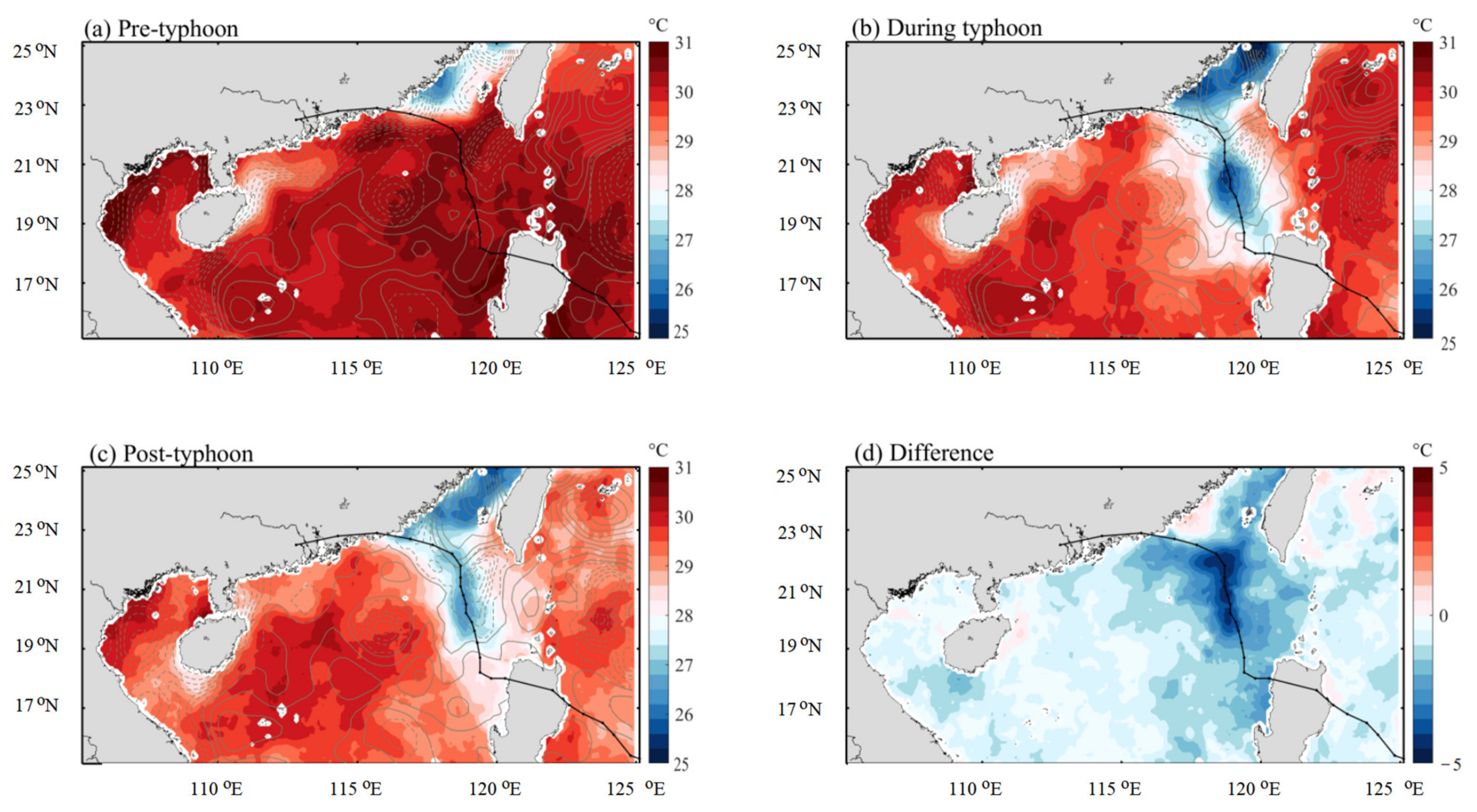
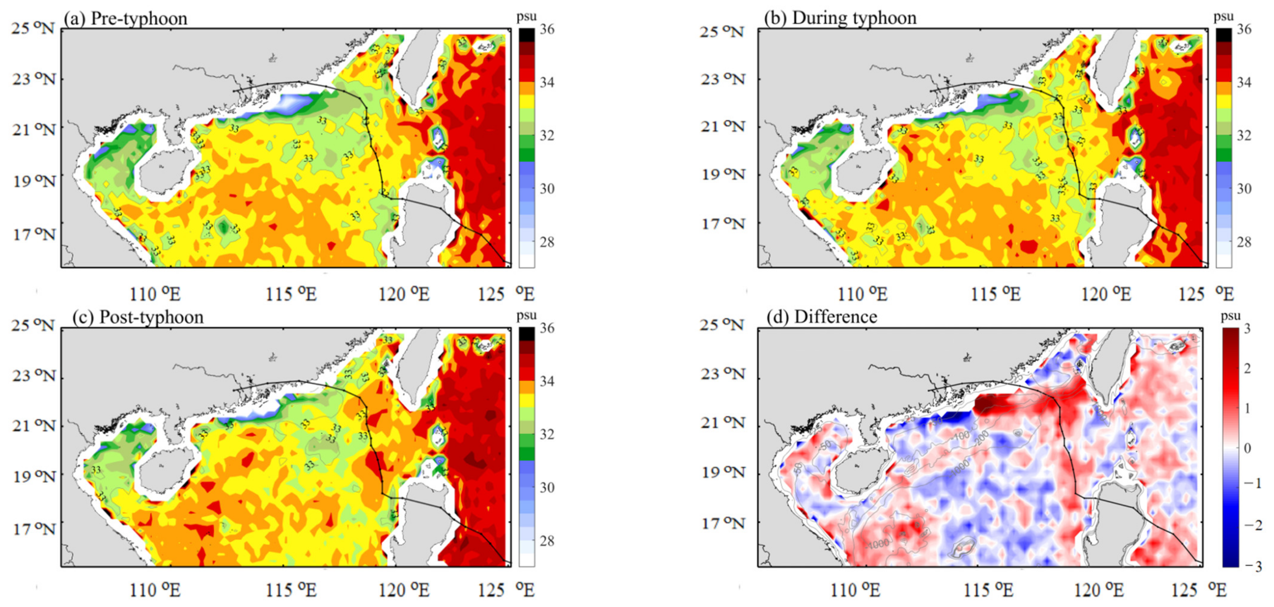
3.3. Distribution of SST and SSS

The most direct ocean response to typhoon Linfa along the path was the SST cooling. Figure 6 shows the variation of the SST before and after the typhoon in the northern SCS. The average SST in the study region before Linfa was 30.1°C, apart from the two costal upwelling regions (Shantou upwelling: 27.4 °C; Hainan upwelling: 28.3 °C). On 5 July 2015, Linfa began to affect the SCS, passing the open ocean with a strong air-sea interaction, thus triggering a dramatic large-scale SST cooling by typhoon-induced upwelling and vertical mixing [52] along the typhoon path. It produced a maximum SST cooling of 4.5 °C near the cold eddy (Figure 6b–d), in agreement with earlier studies [34]. The typhoon slowly moved northward, then turned westward, and the main cooling region (3–4.5 °C) was in the cold eddy and near the inflection point of the path, corresponding to the decreased and increased Chl-a concentrations, respectively. However, high SST appeared in the two coastal upwelling regions, with a sea surface warming of 0.9 °C after the passage of the typhoon (Figure 6d). This is likely attributable to an anomalous northeasterly destroying the traditional coastal upwelling pattern when typhoon invaded south of the upwelling system [43].
Figure 7 displays the variation of sea surface salinity based on SMAP level 3 products during the passage of the typhoon. In the continental shelf region of the northern SCS, the salinity mainly ranged from 26 to 33 psu prior to the arrival of the typhoon (Figure 7a). The lower salinity and high-temperature water stemmed from the nutrient-rich PRP which was transported eastward on the shelf [55] under strong costal currents, and on the open ocean under eddy-entrained currents [15]. The maximum salinity increase was 3 psu in the eastern PRE, while the minimum salinity decrease was 2.6 psu in the western PRE after the passage of typhoon Linfa (Figure 7b–d). This indicated the surface plume water was entrained in the PRE under the weak eastward coastal current, increasing the residence time of freshwater, and then subsequently gradually transported to the western PRE. A large-scale decrease in salinity due to the freshwater from heavy precipitation appeared on the central SCS. An increase in salinity of 0.5–1 psu occurred on both sides of the typhoon path in the open ocean (Figure 7d). This is because strong vertical mixing and upwelling could bring saltier water from the deep ocean to the surface. In addition, decreased salinity appeared in the two coastal upwelling regions, with a decrease of 0.35 psu, corresponding to SST warming after the typhoon (Figure 6d and Figure 7d).

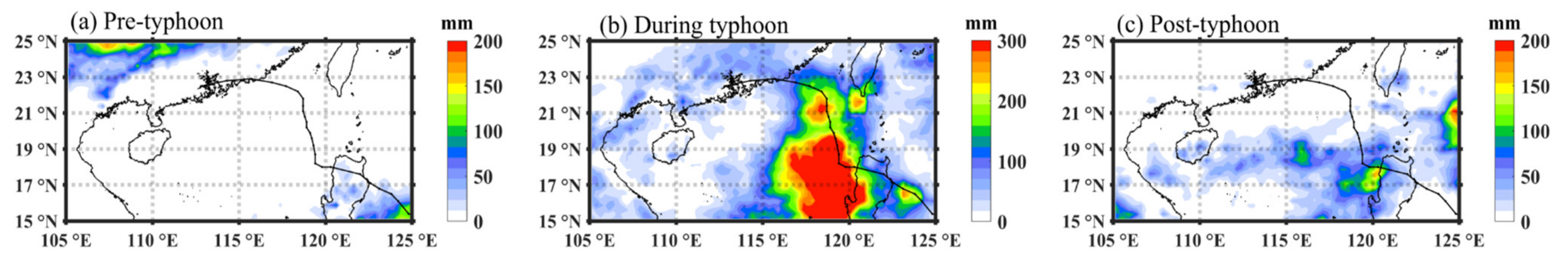
3.4. Distribution of Wind and Rainfall

Prior to the typhoon’s arrival, the southwesterly monsoon was prevailing over the region. The 10 m wind was weak (<8 m/s) during 1–4 July (Figure 8a). During Linfa’s intrusion into the northern SCS, strong winds prevailed over the northeastern SCS, with a maximum wind speed of 16 m/s (Figure 8b–e), whereas the winds over the northwestern SCS promptly decreased (2.8 m/s) (Figure 8b). The favorable southwesterly was clearly substituted with an anomalous northeasterly in the coastal region during 5–9 July.
Before typhoon Linfa, the cumulative rainfall was low (<10 mm) in the northern SCS (Figure 9a). During typhoon Linfa, large-scale rainfall occurred near the typhoon path. The precipitation was remarkably asymmetric, with more (less) cumulative rainfall located on the left (right) of the path, which is consistent with a previous study [57]. The cumulative rainfall (>300 mm) on the left increased by 10–30-fold that before Linfa (Figure 9b). This asymmetry was attributed to the active southwest monsoon over the SCS and topography [57,58]). As the typhoon approached land, the rainfall gradually decreased. The cumulative rainfall (<150 mm) in the coastal region was much less than in the open ocean (Figure 9b). After the typhoon passed, there were still rain belts in the open ocean (Figure 9c). Heavy rainfall can introduce a considerable amount of fresh water into the offshore region, diluting surface salinity.

4. Discussion

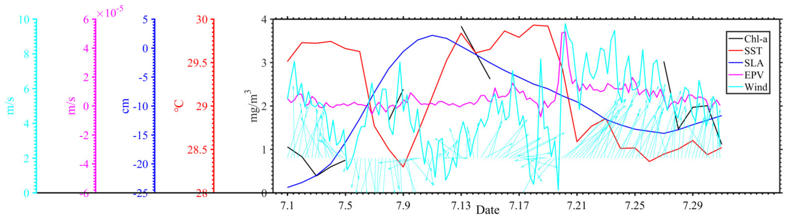
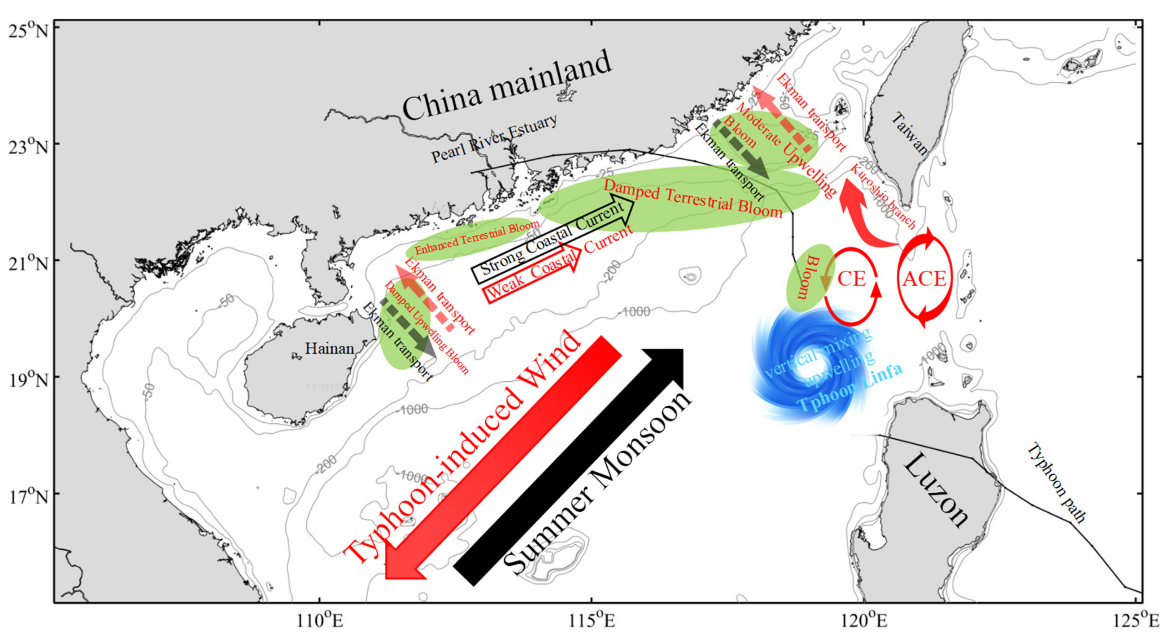
4.1. Typhoon Induced-Upwelling and Mixing

To further explore the influence of the ocean’s internal dynamic mechanisms on phytoplankton blooms, we first estimated the EPV caused by the typhoon. EPV represents the intensity of upwelling: positive EPV indicates upwelling, and negative EPV indicates downing. Before the typhoon, the average EPV in the study region was 4.56 × 10⁻⁶ m/s (Figure 10a). The EPV gradually increased during the typhoon (Figure 10b–h). The average EPV magnitude reached 10−4 within 100 km on both sides of its path, with the maximum value of 2 × 10⁻⁴ m/s appearing at 00:00 UTC on 8 July (Figure 10f), and the EPV then decreased rapidly after the typhoon entered the continental shelf region, with its magnitude being only 10−5 m/s (Figure 10g,h). The integral EPV (IEPV) was calculated to represent the vertical transport distance of subsurface seawater through upwelling (Figure 10i). The stronger IEPV (10–21 m) was in the open ocean where the typhoon passed, rather than in the continental shelf region. The high EIPV region and maximum SST cooling region were essentially located in the same region, corresponding to the slow translational speed. This indicates that the SST cooling was largely the result of the uplifting of cold water (Figure 6d and Figure 10i). The range of IEPV in the continental shelf region was −6 m to 5 m, and presented a tendency of gradually increasing from the nearshore to the offshore regions in the northern SCS (Figure 10i). This suggests that the downwelling dominated the nearshore region, including the two coastal upwelling regions, but the weak upwelling dominated the offshore region.
According to the wind speed at 10 m, a forcing time is obtained by integrating the forced region time [53]. The spatial distribution of forced time and wind work is shown in Figure 11, which was related to typhoon intensity, translation speed, and scale. The range of forced time and wind work within a few hundred kilometers of the typhoon path were 3 h to 45 h and 10 KJ to 70 KJ, respectively, suggesting that a huge input of mechanical energy was introduced into the ocean, and strong mixing could easily occur in the open ocean (Figure 11). Instead, in the continental shelf region, the typhoon quickly moved westward, thereby reducing forcing time and wind work compared to that in open ocean.

4.2. Phytoplankton Bloom in Two Regions

Figure 12 shows that there were three phytoplankton bloom regions, which were located in the open ocean near the typhoon path and the nearshore of the western Pearl River Estuary mouth, and the Shantou-coastal upwelling region. A number of studies [14,21,24,25,27] have illustrated that there has been a strong upwelling and turbulent mixing in the ocean with long forcing time and high IEPV region, which could easily carry nutrient-rich cold water into the mixed layer, promoting phytoplankton growth. Although large-scale, dramatic SST cooling and decreased SLA appeared after the passage of the typhoon, Linfa triggered a two-fold increase in Chl-a, SST cooling (>4 °C), and SLA was reduced 10 cm within a small-scale region in the open ocean, corresponding to strong winds (>15 m/s) and EPV (8 × 10⁻⁵ m/s), rather than those within large-scale regions. The major causes for the difference were ocean stratification, pre-existing nutrient conditions, and typhoon features (intensity and translation speed) [29,30,31]. In addition, a typhoon-enhanced Kuroshio intrusion with denser water may have suppressed typhoon and eddy-induced upwelling, inhibiting nutrient supply [59]. This is probably the reason for phytoplankton blooms appearing in small-scale regions.
The nearshore region was still affected by Linfa even though it was far from the center of the typhoon path, and was associated with weak EPV and winds (Figure 13). The SST was spatially homogeneous, and decreased by 1.2 °C, but salinity and SLA changed markedly along the axial coastline of Guangdong Province after the typhoon (Figure 7 and Figure 13). The sea surface salinity varied from 27 to 31.2 (32.1 to 29.4) psu in the eastern (western) PRE mouth (Figure 7d). Given the duration of the huge discharge of water runoff, combined with the heavy rainfall into the PRE, the moderate northeasterly winds and reduced eastern coastal current modified PRP distribution through onshore Ekman transport (OET), and then modulated phytoplankton distribution patterns. The nutrients in the PRP contributed about 70% of the total annual nutrient load and 80% of the total annual biomass in the shelf waters [4]. The westward extension of PRP could trigger high phytoplankton biomass (increased from 0.72 to 3.1 mg/m3) in the southwestern PRE mouth.
The coastal upwelling region, including the Taiwan Bank (<40 m), and the high Chl-a occurring in summer were caused by the southwest wind and bathymetry-induced upwelling. The shift in wind directions associated with the typhoon intrusion south of the upwelling system could destroy the upwelling patterns and give rise to OET, corresponding to increasing SLA. Subsequently, the strong cyclonic wind stress induced vertical mixing, which alters water stratification, resulting in significant SST cooling and the resuspension of seabed sediments, which increase SPM concentration and nutrient supply (Figure 14). Light is the major regulator of biological production. The high turbidity caused by enhanced vertical mixing can suppress phytoplankton growth [40,60,61]. This is the reason why Chl-a concentration did not significantly change between the pre-typhoon period and 10 July. Given that the phytoplankton responses to external nutrient inputs were not strong when the phytoplankton was already growing in nutrient replete conditions [62], the Chl-a concentrations ultimately increased by 38% (from 0.86 to 1.26) 4 days after the typhoon passed, which is far less than the magnitude of its increases in other bloom regions (Figure 14).

4.3. Phytoplankton Decline in the Two Regions

The Chl-a concentration strikingly decreased after the typhoon’s passage in the continental shelf region (reduced by about 3-fold) and in the upwelling region (reduced by about 3.5-fold), especially in the two regions southeastern the PRE (around the typhoon path) and in the eastern Leizhou Peninsula.
During June and July, because of the strong river discharge, nutrient enrichment in the plume stretched over a broad extent of the shelf during the summer monsoon, and this produced significant biomass on the continental shelf of the northeastern SCS, where low salinity, high temperatures, and high SPM appeared (Figure 5, Figure 6 and Figure 7). As the typhoon entered the SCS, the southwest monsoon turned to the northwest, which lasted for 4 days. The northeasterly wind induced-Ekman transport led to increased salinity and SLA, and a weaker eastern coastal current in the eastern PRE mouth. This may suppress the nutrient supply from the river discharge [11]. The SST cooling and decreased SLA corresponded to reduced Chl-a and increased wind and EPV in both the eastern PRE mouth and in the continental shelf region where the typhoon passed (Figure 15). Due to the strong ocean stratification caused by the PRE plume and rainfall, which may suppress vertical mixing and upwelling, the intensity of the vertical mixing and upwelling was weak compared to that in the open ocean. Therefore, the typhoon induced-upwelling, vertical mixing, and horizontal advection were not enough to lift deep nutrient-rich water to the surface layer, but further reduced pre-existing, nutrient-rich water in the surface layer when the typhoon passed though the continental shelf. These data suggest that the decayed coastal current inhibiting the nutrient supply and the typhoon directly reducing the nutrient supply were significant factors for the phytoplankton decline. In nearshore regions, light conditions caused by the high turbidity after the typhoon are considered to be a factor affecting the phytoplankton biomass [63]. In addition to nutrient conditions, the pre-existing vertical distribution of phytoplankton determine the response of Chl-a concentrations under typhoon conditions. Qiu et al. [41] demonstrated that strong vertical mixing caused by typhoon Nangka led to a sudden decrease in the phytoplankton abundance in surface water near the PRE environment. As proposed by Mao et al. [45], it was found that the vertical distribution of phytoplankton in 196 seawater samples gradually decreased in abundance with increasing depth in the northeastern SCS. After typhoon Haitang, the total phytoplankton cell abundance (e.g., Cyanophyta) in the surface layer was significantly reduced, and cell abundance in the subsurface layer did not change significantly [45]. Consequently, the phytoplankton decline was attributed to OET-interrupted nutrient supply, accompanied by the vertical redistribution of phytoplankton with reduced nutrients, by typhoon induced physical processes. Other factors, however, may also play roles in the phytoplankton decline. The enhanced Kuroshio intrusion into the northeastern SCS happened under typhoon conditions (Figure 5d). The Kuroshio intrusion water, with high salinity and few nutrients, was able to inhibit nutrient uplift driving by typhoon-induced vertical mixing and upwelling [59], thus resulting in phytoplankton decline.
The coastal upwelling region, the eastern Leizhou Peninsula, was affected by typhoon Linfa’s peripheral wind field. As shown in Figure 16, the SST, wind speed, and EPV did not change significantly, but the Chl-a concentrations were reduced by about 3.5-fold. The typhoon-induced abnormal wind vectors were opposite to the summer monsoon, giving rise to offshore Ekman transport, which subsequently gradually weakened, eventually being replaced by OET [28,43]. The role of OET and the weak northern coastal current was to reduce the nutrient supply from terrestrial sources and increase SLA, thereby leading to phytoplankton decline.

5. Conclusions

Based on the multi-satellite datasets, we presented here the significant biophysical changes in the northern SCS during the passage of typhoon Linfa. Typhoon Linfa gave rise to two phytoplankton declines and three phytoplankton blooms in the northern SCS. The phytoplankton dynamics are summarized in Figure 17. The phytoplankton declined in two regions: the continental shelf region where the typhoon passed and the eastern Leizhou Peninsula. Due to the huge freshwater discharge and the sediment discharge from the PRE prior to the arrival of typhoon Linfa, phytoplankton bloom events with high SPM frequently occurred in the continental shelf region, which may have led to high (low) phytoplankton abundance in surface (subsurface) layer. Afterwards, the continental shelf phytoplankton decline was mainly caused by the nutrient reduction induced by the decayed northeastern coastal current, OET, and Kuroshio intrusion water, combined with the uplifted subsurface of low Chl-a, driven by typhoon-induced vertical mixing and upwelling. The eastern Leizhou Peninsula coastal upwelling region phytoplankton decline was attributed to reduced nutrients, triggered by OET and the decayed northern coastal current. In addition, three phytoplankton blooms were observed during the post-typhoon period: in the open ocean where the typhoon passed, in the coastal upwelling region of northeastern Guangdong, and in the southwestern PRE mouth. First, nutrient uplifting caused by strong mixing and upwelling contributed to the small-scale blooms in the open ocean. Second, the northeasterly winds and reduced northeastern coastal current could result in the westward extension of PRP, thereby triggering high phytoplankton biomass in the southwestern PRE mouth. Finally, in the coastal upwelling region, the phytoplankton responses to external nutrient inputs were not strong when phytoplankton was already growing in nutrient-replete conditions. OET and the high turbidity induced by enhanced vertical mixing barely gave rise to a moderate phytoplankton bloom.
It remains uncertain whether climate change would lead to an increase in the number of typhoons, but there is more confidence that warmer ocean temperatures and higher sea levels are expected to intensify. The strong winds associated with typhoons initiate intense upwelling and mixing, which results in the enhancement of phytoplankton biomass in the open ocean after the passage of typhoons. Presently, the quantitative estimation of the response of phytoplankton dynamics to typhoons in the northern SCS is difficult because satellite data can only reflect surface conditions. Further in situ observations and model simulations are required to explain the role that typhoons play in enhancing or reducing phytoplankton abundance.

Author Contributions

Conceptualization, T.W. and S.Z.; methodology T.W. and S.Z.; software, T.W.; validation, T.W. and S.Z.; formal analysis, T.W. and S.Z.; investigation, T.W.; resources, T.W.; data curation, T.W. and S.Z.; writing—original draft preparation, T.W.; writing—review and editing, S.Z.; visualization, T.W.; supervision, S.Z.; project administration, S.Z.; funding acquisition, S.Z. Both authors have read and agreed to the published version of the manuscript.

Funding

This work was supported by the National Natural Science Foundation of China (U1901213, 41676008, 40876005 and 41376035), the Innovation and Entrepreneurship Project of Shantou (2021112176541391), and the Scientific Research Start-Up Fund of Shantou University (NTF20006).

Institutional Review Board Statement

Not applicable.

Informed Consent Statement

Not applicable.

Data Availability Statement

We thank the Remote Sensing System for providing sea surface temperature, salinity, 10 m wind (ftp://ftp.remss.com/ accessed on 1 May 2021), GlobColor’s Working Group for Chl-a data (http://hermes.acri.fr accessed on 1 May 2021), and NASA for daily precipitation. Suspended Particulate Matter Surface, level anomaly, and geostrophic current data in this study were provided freely by Copernicus Marine Environment Monitoring Service (CMEMS, http://marine.copernicus.eu/ accessed on 1 May 2021).

Acknowledgments

We would like to thank the anonymous reviewers for their helpful comments on improving the manuscript.

Conflicts of Interest

The authors declare no conflict of interest.

References

  1. Zhu, Y.; Sun, J.; Wang, Y.; Li, S.; Xu, T.; Wei, Z.; Qu, T. Overview of the multi-layer circulation in the South China Sea. Prog. Oceanogr. 2019, 175, 171–182. [Google Scholar] [CrossRef]
  2. Wong, G.T.; Pan, X.; Li, K.Y.; Shiah, F.K.; Ho, T.Y.; Guo, X. Hydrography and nutrient dynamics in the northern South China sea Shelf-sea (NoSoCS). Deep Sea Res. Part II Top. Stud. Oceanogr. 2015, 117, 23–40. [Google Scholar] [CrossRef]
  3. Han, A.; Dai, M.; Kao, S.J.; Gan, J.; Li, Q.; Wang, L.; Zhai, W.; Wang, L. Nutrient dynamics and biological consumption in a large continental shelf system under the influence of both a river plume and coastal upwelling. Limnol. Oceanogr. 2012, 57, 486–502. [Google Scholar] [CrossRef] [Green Version]
  4. Gan, J.; Lu, Z.; Dai, M.; Cheung, A.Y.; Liu, H.; Harrison, P. Biological response to intensified upwelling and to a river plume in the northeastern South China Sea: A modeling study. J. Geophys. Res. Oceans. 2010, 115, C09001. [Google Scholar] [CrossRef]
  5. Lu, Z.; Gan, J. Controls of seasonal variability of phytoplankton blooms in the Pearl River Estuary. Deep Sea Res. Part II Top. Stud. Oceanogr. 2015, 117, 86–96. [Google Scholar] [CrossRef]
  6. Huang, X.P.; Huang, L.M.; Yue, W.Z. The characteristics of nutrients and eutrophication in the Pearl River estuary, South China. Mar. Pollut. Bull. 2003, 47, 30–36. [Google Scholar] [CrossRef]
  7. Zhai, W.; Dai, M.; Cai, W.-J.; Wang, Y.; Wang, Z. High partial pressure of CO2 and its maintaining mechanism in a subtropical estuary: The Pearl River estuary, China. Mar. Chem. 2005, 93, 21–32. [Google Scholar] [CrossRef]
  8. Zhang, S.; Lu, X.X.; Higgitt, D.L.; Chen, C.T.A.; Han, J.; Sun, H. Recent changes of water discharge and sediment load in the Zhujiang (Pearl River) Basin, China. Glob. Environ. Chang. 2008, 60, 365–380. [Google Scholar] [CrossRef]
  9. Shu, Y.; Wang, D.; Zhu, J.; Peng, S. The 4-D structure of upwelling and Pearl River plume in the northern South China Sea during summer 2008 revealed by a data assimilation model. Ocean Modell. 2011, 36, 228–241. [Google Scholar] [CrossRef]
  10. Wang, D.; Zhuang, W.; Xie, S.P.; Hu, J.; Shu, Y.; Wu, R. Coastal upwelling in summer 2000 in the northeastern South China Sea. J. Geophys. Res. Oceans. 2012, 117, C04009. [Google Scholar] [CrossRef] [Green Version]
  11. Lu, Z.; Gan, J.; Dai, M.; Cheung, A.Y. The influence of coastal upwelling and a river plume on the subsurface chlorophyll maximum over the shelf of the northeastern South China Sea. J. Mar. Syst. 2010, 82, 35–46. [Google Scholar] [CrossRef]
  12. Chen, Z.; Pan, J.; Jiang, Y.; Lin, H. Far-reaching transport of Pearl River plume water by upwelling jet in the northeastern South China Sea. J. Mar. Syst. 2017, 173, 60–69. [Google Scholar] [CrossRef]
  13. Xue, H.J.; Chai, F. Coupled physical-biological model for the Pearl River Estuary: A phosphate limited subtropical ecosystem. In Estuarine and Coastal Modeling (2001); American Society of Civil Engineers: Reston, VA, USA, 2002; pp. 913–928. [Google Scholar]
  14. Zheng, G.M.; Tang, D. Offshore and nearshore chlorophyll increases induced by typhoon winds and subsequent terrestrial rainwater runoff. Mar. Ecol Prog. Ser. 2007, 333, 61–74. [Google Scholar] [CrossRef] [Green Version]
  15. He, X.; Xu, D.; Bai, Y.; Pan, D.; Chen, C.T.A.; Chen, X.; Gong, F. Eddy-entrained Pearl River plume into the oligotrophic basin of the South China Sea. Cont. Shelf. Res. 2016, 124, 117–124. [Google Scholar] [CrossRef]
  16. Jing, Z.Y.; Qi, Y.Q.; Hua, Z.L.; Zhang, H. Numerical study on the summer upwelling system in the northern continental shelf of the South China Sea. Cont. Shelf. Res. 2009, 29, 467–478. [Google Scholar] [CrossRef] [Green Version]
  17. Lü, X.; Qiao, F.; Wang, G.; Xia, C.; Yuan, Y. Upwelling off the west coast of Hainan Island in summer: Its detection and mechanisms. Geophys. Res. Lett. 2008, 35, L02604. [Google Scholar] [CrossRef]
  18. Wang, D.; Shu, Y.; Xue, H.; Hu, J.; Chen, J.; Zhuang, W.; Zu, T.; Xu, J. Relative contributions of local wind and topography to the coastal upwelling intensity in the northern South China Sea. J. Geophys. Res. Oceans. 2014, 119, 2550–2567. [Google Scholar] [CrossRef]
  19. Forryan, A.; Garabato, A.C.N.; Vic, C.; Nurser, A.G.; Hearn, A.R. Galápagos upwelling driven by localized wind–front interactions. Sci. Rep. 2021, 11, 1–12. [Google Scholar] [CrossRef]
  20. Liu, K.S.; Chan, J.C. Recent increase in extreme intensity of tropical cyclones making landfall in South China. Clim. Dyn. 2020, 55, 1059–1074. [Google Scholar] [CrossRef]
  21. Lin, I.; Liu, W.T.; Wu, C.C.; Wong, G.T.; Hu, C.; Chen, Z.; Liang, D.-W.; Yang, Y.; Liu, K.K. New evidence for enhanced ocean primary production triggered by tropical cyclone. Geophys. Res. Lett. 2003, 30, 1718. [Google Scholar] [CrossRef] [Green Version]
  22. Huang, S.M.; Oey, L.Y. Right-side cooling and phytoplankton bloom in the wake of a tropical cyclone. J. Geophys. Res. Oceans 2015, 120, 5735–5748. [Google Scholar] [CrossRef]
  23. Lin, Y.C.; Oey, L.Y. Rainfall-enhanced blooming in typhoon wakes. Sci. Rep. 2016, 6, 31310. [Google Scholar] [CrossRef] [Green Version]
  24. Pan, G.; Chai, F.; Tang, D.; Wang, D. Marine phytoplankton biomass responses to typhoon events in the South China Sea based on physical-biogeochemical model. Ecol. Modell. 2017, 356, 38–47. [Google Scholar] [CrossRef]
  25. Wang, T.; Zhang, S.; Chen, F.; Ma, Y.; Jiang, C.; Yu, J. Influence of sequential tropical cyclones on phytoplankton blooms in the northwestern South China Sea. J. Oceanol. Limnol. 2021, 39, 14–25. [Google Scholar] [CrossRef]
  26. Zhao, H.; Tang, D.; Wang, D. Phytoplankton blooms near the Pearl River estuary induced by Typhoon Nuri. J. Geophys. Res. Oceans 2009, 114, C12027. [Google Scholar] [CrossRef]
  27. Liu, Y.; Tang, D.; Evgeny, M. Chlorophyll concentration response to the typhoon wind-pump induced upper ocean processes considering air–sea heat exchange. Remote Sens. 2019, 11, 1825. [Google Scholar] [CrossRef] [Green Version]
  28. Liu, S.; Li, J.; Sun, L.; Wang, G.; Tang, D.; Huang, P.; Yan, H.; Gao, S.; Liu, C.; Gao, Z. Basin-wide responses of the South China sea environment to super typhoon mangkhut (2018). Sci. Total Environ. 2020, 731, 139093. [Google Scholar] [CrossRef] [PubMed]
  29. Wang, Y. Composite of typhoon-induced sea surface temperature and chlorophyll-a responses in the South China Sea. J. Geophys. Res. Oceans 2020, 125, e2020JC016243. [Google Scholar] [CrossRef]
  30. Liu, F.; Tang, S. Influence of the interaction between typhoons and oceanic mesoscale eddies on phytoplankton blooms. J. Geophys. Res. Oceans 2018, 123, 2785–2794. [Google Scholar] [CrossRef]
  31. Xu, F.; Yao, Y.; Oey, L.; Lin, Y. Impacts of pre-existing ocean cyclonic circulation on sea surface chlorophyll-a concentrations off northeastern Taiwan following episodic typhoon passages. J. Geophys. Res. Oceans 2017, 122, 6482–6497. [Google Scholar] [CrossRef]
  32. Babin, S.M.; Carton, J.A.; Dickey, T.D.; Wiggert, J.D. Satellite evidence of hurricane-induced phytoplankton blooms in an oceanic desert. J. Geophys. Res. Oceans 2004, 109, C03043. [Google Scholar] [CrossRef]
  33. Kuttippurath, J.; Sunanda, N.; Martin, M.V.; Chakraborty, K. Tropical storms trigger phytoplankton blooms in the deserts of north Indian Ocean. NPJ Clim. Atmos. Sci. 2021, 4, 1–12. [Google Scholar] [CrossRef]
  34. Sun, L.; Yang, Y.J.; Xian, T.; Lu, Z.M.; Fu, Y.F. Strong enhancement of chlorophyll a concentration by a weak typhoon. Mar. Ecol Prog. Ser. 2010, 404, 39–50. [Google Scholar] [CrossRef]
  35. Ye, H.J.; Sui, Y.; Tang, D.L.; Afanasyev, Y.D. A subsurface chlorophyll a bloom induced by typhoon in the South China Sea. J. Mar. Syst. 2013, 128, 138–145. [Google Scholar] [CrossRef]
  36. Lee, J.H.; Moon, J.H.; Kim, T. Typhoon-triggered phytoplankton bloom and associated upper-ocean conditions in the northwestern Pacific: Evidence from satellite remote sensing, Argo profile, and an ocean circulation model. J. Mar. Sci. Eng. 2020, 8, 788. [Google Scholar] [CrossRef]
  37. Zhao, H.; Han, G.; Zhang, S.; Wang, D. Two phytoplankton blooms near Luzon Strait generated by lingering Typhoon Parma. J. Geophys. Res. Biogeosci. 2013, 118, 412–421. [Google Scholar] [CrossRef]
  38. Chai, F.; Wang, Y.; Xing, X.; Yan, Y.; Xue, H.; Wells, M.; Boss, E. A limited effect of sub-tropical typhoons on phytoplankton dynamics. Biogeosciences 2021, 18, 849–859. [Google Scholar] [CrossRef]
  39. Lin, I.I. Typhoon-induced phytoplankton blooms and primary productivity increase in the western North Pacific subtropical ocean. J. Geophys. Res. Oceans 2012, 117, C03039. [Google Scholar] [CrossRef]
  40. Li, Y.; Ye, X.; Wang, A.; Li, H.; Chen, J.; Qiao, L. Impact of Typhoon Morakot on chlorophyll a distribution on the inner shelf of the East China Sea. Mar. Ecol Prog. Ser. 2013, 483, 19–29. [Google Scholar] [CrossRef] [Green Version]
  41. Qiu, D.; Zhong, Y.; Chen, Y.; Tan, Y.; Song, X.; Huang, L. Short-term phytoplankton dynamics during typhoon season in and near the Pearl River Estuary, South China Sea. J. Geophys. Res. Biogeosci. 2019, 124, 274–292. [Google Scholar] [CrossRef]
  42. Chang, J.; Chung, C.; Gong, G. Influences of cyclones on chlorophyll a concentration and Synechococcus abundance in a subtropical western Pacific coastal ecosystem. Oceanogr. Lit. Rev. 1997, 4, 346. [Google Scholar] [CrossRef] [Green Version]
  43. Pan, A.; Guo, X.; Xu, J.; Huang, J.; Wan, X. Responses of Guangdong coastal upwelling to the summertime typhoons of 2006. Sci. China Earth Sci. 2012, 55, 495–506. [Google Scholar] [CrossRef]
  44. Shen, D.; Li, X.; Wang, J.; Bao, S.; Pietrafesa, L.J. Dynamical Ocean responses to Typhoon Malakas (2016) in the vicinity of Taiwan. J. Geophys. Res. Oceans 2021, 126, e2020JC016663. [Google Scholar] [CrossRef]
  45. Mao, Y.; Sun, J.; Guo, C.; Wei, Y.; Wang, X.; Yang, S.; Wu, C. Effects of typhoon Roke and Haitang on phytoplankton community structure in northeastern South China Sea. Ecosyst. Health Sust. 2019, 5, 144–154. [Google Scholar] [CrossRef] [Green Version]
  46. Gohin, F. Annual cycles of chlorophyll-a, non-algal suspended particulate matter, and turbidity observed from space and in-situ in coastal waters. Ocean Sci. 2011, 7, 705–732. [Google Scholar] [CrossRef] [Green Version]
  47. Wentz, F.J.; Gentemann, C.; Smith, D.; Chelton, D. Satellite measurements of sea surface temperature through clouds. Science 2000, 288, 847–850. [Google Scholar] [CrossRef] [PubMed] [Green Version]
  48. Gentemann, C.L.; Wentz, F.J.; Mears, C.A.; Smith, D.K. In-Situ validation of Tropical Rainfall Measuring Mission microwave sea surface temperatures. J. Geophys. Res. Oceans 2004, 109, C04021. [Google Scholar] [CrossRef] [Green Version]
  49. Meissner, T.; Wentz, F.J.; Le Vine, D.M. The Salinity Retrieval Algorithms for the NASA Aquarius Version 5 and SMAP Version 3 Releases. Remote Sens. 2018, 10, 1121. [Google Scholar] [CrossRef] [Green Version]
  50. Atlas, R.; Hoffman, R.N.; Ardizzone, J.; Leidner, S.M.; Jusem, J.C.; Smith, D.K.; Gombos, D. A cross-calibrated, multiplatform ocean surface wind velocity product for meteorological and oceanographic applications. Bull. Am. Meteorol. Soc. 2011, 92, 157–174. [Google Scholar] [CrossRef]
  51. Huffman, G.J.; Adler, R.F.; Bolvin, D.T.; Nelkin, E.J. The TRMM multi-satellite precipitation analysis (TMPA). In Satellite Rainfall Applications for Surface Hydrology; Springer: Dordrecht, The Netherlands, 2010; pp. 3–22. [Google Scholar] [CrossRef] [Green Version]
  52. Price, J.F. Upper Ocean response to a hurricane. J. Phys. Oceanogr. 1981, 11, 153–175. [Google Scholar] [CrossRef] [Green Version]
  53. Sun, L.; Li, Y.X.; Yang, Y.J.; Wu, Q.; Chen, X.T.; Li, Q.Y.; Li, Y.-B.; Xian, T. Effects of super typhoons on cyclonic ocean eddies in the western North Pacific: A satellite data-based evaluation between 2000 and 2008. J. Geophys. Res. Oceans 2014, 119, 5585–5598. [Google Scholar] [CrossRef]
  54. Mei, W.; Pasquero, C.; Primeau, F. The effect of translation speed upon the intensity of tropical cyclones over the tropical ocean. Geophys. Res. Lett. 2012, 39, L07801. [Google Scholar] [CrossRef] [Green Version]
  55. Gan, J.; Li, L.; Wang, D.; Guo, X. Interaction of a river plume with coastal upwelling in the northeastern South China Sea. Cont. Shelf. Res. 2009, 29, 728–740. [Google Scholar] [CrossRef]
  56. Bai, Y.; Huang, T.H.; He, X.; Wang, S.L.; Hsin, Y.C.; Wu, C.R.; Zhai, W.; Lui, H.-T.; Chen, C.T.A. Intrusion of the Pearl River plume into the main channel of the Taiwan Strait in summer. J. Sea Res. 2015, 95, 1–15. [Google Scholar] [CrossRef]
  57. Xu, W.; Jiang, H.; Kang, X. Rainfall asymmetries of tropical cyclones prior to, during, and after making landfall in South China and Southeast United States. Atmos. Res. 2014, 139, 18–26. [Google Scholar] [CrossRef]
  58. Klotz, B.W.; Jiang, H. Examination of surface wind asymmetries in tropical cyclones. Part I: General structure and wind shear impacts. Mon. Weather Rev. 2017, 145, 3989–4009. [Google Scholar] [CrossRef]
  59. Liu, Y.; Tang, D.; Tang, S.; Morozov, E.; Liang, W.; Sui, Y. A case study of Chlorophyll a response to tropical cyclone Wind Pump considering Kuroshio invasion and air-sea heat exchange. Sci. Total Environ. 2020, 741, 140290. [Google Scholar] [CrossRef]
  60. Domingues, R.B.; Guerra, C.C.; Barbosa, A.B.; Galvao, H.M. Are nutrients and light limiting summer phytoplankton in a temperate coastal lagoon? Aquatic Ecol. 2015, 49, 127–146. [Google Scholar] [CrossRef]
  61. Pennock, J.R.; Sharp, J.H. Temporal alternation between light-and nutrient imitation of phytoplankton production in a coastal plain estuary. Mar. Ecol. Prog. Ser. 1994, 111, 275–288. [Google Scholar] [CrossRef]
  62. Teixeira, I.G.; Arbones, B.; Froján, M.; Nieto-Cid, M.; Álvarez-Salgado, X.A.; Castro, C.G.; Fernández, E.; Sobrino, C.; Teira, E.; Figueiras, F.G. Response of phytoplankton to enhanced atmospheric and riverine nutrient inputs in a coastal upwelling embayment. Estuar. Coast. Shelf Sci. 2018, 210, 132–141. [Google Scholar] [CrossRef]
  63. Dokulil, M.T. Environmental control of phytoplankton productivity in turbulent turbid systems. In Phytoplankton in Turbid Environments: Rivers and Shallow Lakes; Springer: Dordrecht, The Netherlands, 1994; pp. 65–72. [Google Scholar] [CrossRef]
Figure 1. Typhoon path in the northern SCS. The colored dots indicate the center of typhoon with 6-h interval. The red triangle denotes Gaoyao station.
Jmse 09 00794 g001
Figure 2. Time series of typhoon intensity and transition speed.
Jmse 09 00794 g002
Figure 3. Spatial distribution of Chlorophyll-a (ac) and SPM (df) concentrations during pre-typhoon (one week) and post-typhoon (one week). The gray line represents the water depth (25 m, 50 m, 100 m, 200 m, 1000 m). The black line denotes typhoon path.
Jmse 09 00794 g003
Figure 4. Time series of monthly runoff (unit: billion cubic meters) (blue) and sediment runoff (unit: ten thousand tons) (orange) at Gaoyao hydrological station during the 2015 year.
Jmse 09 00794 g004
Figure 5. Spatial distribution of sea level anomaly (shading) and geostrophic current (arrow) during pre-typhoon (a) 1–5 July, during typhoon (b) 6–9 July, and post-typhoon (c) 10–12 July, and difference (d) 10–12 July minus 1–5 July. The black line denotes typhoon path.
Jmse 09 00794 g005
Figure 6. Spatial distribution of sea surface temperature during pre-typhoon (a) 1–5 July, during typhoon (b) 6–9 July, and post-typhoon (c) 10–12 July, and difference (d) 10–12 July minus 1–5 July. The gray line represents the sea level anomaly. The black line denotes typhoon path.
Jmse 09 00794 g006
Figure 7. Spatial distribution of sea surface salinity during pre-typhoon (a) 1–5 July, during typhoon (b) 6–9 July, and post-typhoon (c) 10–12 July, and difference (d) 10–12 July minus 1–5 July. The gray line represents the water depth (25 m, 50 m, 100 m, 200 m, 1000 m). The black line denotes the typhoon path.
Jmse 09 00794 g007
Figure 8. Spatial distribution of 10 m wind vector (arrows) and wind speed (shading) during pre-typhoon (a) 1–4 July and on 5 July (b), 6 July (c), 7 July (d), 8 July (e), 9 July (f). The black line denotes typhoon path.
Jmse 09 00794 g008
Figure 9. Spatial distribution of cumulative rainfall during pre-typhoon (a) 1–4 July, during typhoon (b) 5–9 July, and post-typhoon (c) 10–13 July. The black line denotes typhoon path.
Jmse 09 00794 g009
Figure 10. Spatial distribution of 10 m wind vector (arrows) and Ekman pumping velocity (shading) during pre-typhoon (a) 1–4 July, on 12UTC 5 July (b), 12UTC 6 July (c), 12UTC 7 July (d), 18UTC 7 July (e), 00UTC 8 July (f), 12UTC 8 July (g), 00UTC 9 July (h) and 00UTC 9 July (i), and Integer Ekman pumping velocity. The black line denotes typhoon path.
Jmse 09 00794 g010
Figure 11. Spatial distribution of forcing time (arrows) and wind work (shading) during typhoon Linfa. The black line denotes typhoon path.
Jmse 09 00794 g011
Figure 12. Time series of Chl-a concentration, sea surface temperature, sea level anomaly, Ekman pumping velocity, and wind speed (vector) in the open ocean where the typhoon passed.
Jmse 09 00794 g012
Figure 13. Time series of Chl-a concentration, sea surface temperature, sea level anomaly, Ekman pumping velocity and wind speed (vector) in the nearshore region of PRE mouth.
Jmse 09 00794 g013
Figure 14. Time series of Chl-a concentration, sea surface temperature, sea level anomaly, Ekman pumping velocity, and wind speed (vector) in the coastal upwelling region–Shantou.
Jmse 09 00794 g014
Figure 15. Time series of Chl-a concentration, sea surface temperature, sea level anomaly, Ekman pumping velocity, and wind speed (vector) in the continental shelf region where the typhoon passed.
Jmse 09 00794 g015
Figure 16. Time series of Chl-a concentration, sea surface temperature, sea level anomaly, Ekman pumping velocity, and wind speed (vector) in the coastal upwelling region–the eastern Leizhou Peninsula.
Jmse 09 00794 g016
Figure 17. Schematic diagram illustrating phytoplankton dynamics in the northern SCS during the passage of typhoon Linfa.
Jmse 09 00794 g017
Publisher’s Note: MDPI stays neutral with regard to jurisdictional claims in published maps and institutional affiliations.

