1. Introduction
Spain is the European Union country with the longest coastline, with a length of 8000 km. It is also the closest European country to the axis of one of the world’s major maritime routes. Its geographical location positions it as a strategic element in international shipping and a logistics platform in Southern Europe.
The Spanish Port System includes 46 ports of general interest. The importance of ports in the Spanish economy, as links in the logistics and transport chains, is reflected in the following figures [
1]:
They handle nearly 60% of exports and 85% of imports, accounting for 53% of Spanish foreign trade with the European Union and 96% with third countries.
The state port system’s activity contributes to nearly 20% of the transport sector’s GDP, accounting for 1.1% of the Spanish GDP.
It employs more than 35,000 workers directly and around 110,000 indirectly.
These figures reveal that events that could disrupt the normal operations of a port and actions aimed to improve or optimize processes can have a significant economic impact. Port infrastructures are subject to different meteorological conditions such as waves, wind, and currents that can produce such disruptions. We can classify these conditions into extreme and normal ones. When these conditions are extreme (extreme range regime), the only way to minimize the negative impact is to build infrastructures that ensure the structural integrity of the port. Usually, regular ship operations (berthing, loading, and unloading) are not possible in this regime. However, in normal meteorological and ocean conditions, the port must minimize the effect of climate forcers on ship movements, ensuring that they can operate safely.
Port operability is usually quantified based on the movements of moored ships. When a vessel experiences large movements during its stay in port, these harm the operation, causing delays or even operational stoppages, with the corresponding economic cost. There are numerous regulations and recommendations that propose limits for the amplitudes of the movements compatible with the operation [
2,
3,
4,
5].
It is important to note that these criteria represent generic values applicable to port facilities worldwide, which in most cases have been established based on subjective observations of operators and shipmasters, without particularized studies to support them. The general nature of these criteria means that they are not adequately adjusted to the characteristics of each port facility, and it would therefore be advisable to make them more specific.
The variables involved in the moored vessel movement are mainly of two different types. In first place, there are the aforementioned ocean-meteorological conditions. Secondly, there are the variables related to the infrastructure, the ship and the port. The same weather conditions affect the vessel movement differently, depending on the size of the ship, the state of the cargo and the type of mooring, among others. Thus, the relationship between the variables is complex and, consequently, difficult to obtain.
In order to obtain the movement of a vessel, we can follow two approaches. One of them is using a physical or numerical model of a vessel and the port infrastructure and using physical or numerical simulations of the ocean-meteorological variables that influence the vessel movement and their interaction with the vessel and the infrastructure, obtaining the vessel movements. As mentioned in [
6,
7], this approach has a series of limitations. Physical modeling was one of the most widely used techniques to analyze the vessel behavior, the operational conditions [
8,
9] and to quantify the influence of mooring tension and fender stiffness on the operability of a berth [
10,
11]. However, it has several limitations:
It is a simplified reproduction of reality.
The construction and calibration processes must be highly meticulous, generating a high economic and time cost.
This methodology is very rigid from modifications of test configuration (mooring configuration, fender stiffness, mooring tension and type vessel).
Numerical modeling of the moored vessel is another widely used methodology. In the past decades, its evolution has allowed it to be a viable alternative to physical modeling [
12,
13,
14,
15]. Cummins proposed the mathematical description of this phenomenon [
16]. The main advantage of this tool is its high adaptability to changes in the geometry, the wave conditions or the vessel type. However, it has some limitations; firstly, the hypotheses adopted for solving the equations, generating certain deviations from reality. Furthermore, their validation is usually carried out using data from physical modeling [
17] and not with real data. Finally, it does not reproduce the variations experienced by the ship during the operation.
The field campaign is the third alternative for the moored vessel’s analysis. It is the least explored methodology despite providing very relevant information on the vessel’s operation reality. The main reason is related to the high economic cost of the monitoring equipment and the personnel required to carry out extensive field campaigns containing a large number of ships. The most widespread measurement technology currently used is the GPS-RTK system [
18,
19,
20]. Another frequently used technology is laser equipment [
21]. There are only two examples where an extensive monitoring campaign was carried out with different vessel typologies during operation [
22,
23]. During the past decades, this type of work has focused mainly on the study of the long wave [
21,
24,
25,
26] and to validate physical or numerical models [
13,
27].
Currently, several ports of authority throughout Europe, such as Algeciras, A Coruña, or Rotterdam, are involved in the R+D+i projects for the analysis of the interaction between the physical environment, the behavior of the ship and the berthing infrastructure. Their main objective is to develop advanced management tools that help identify and predict possible risk situations and, therefore, replant operations and the allocation of resources to offer the desired level of service or to reinforce port safety and security measures. This work followed the latter approach to obtain a dataset large enough (with at least several hundred hours of recorded ships movements) and use it to create several machine learning-based prediction models that predict the different vessel movements. The purpose of these models is to predict how a vessel will move before it is operating. When the models predict that the vessel movements are excessive for loading and unloading cargo, port operators can decide to take actions that reduce the vessel movements. For instance, they could change the mooring arrangement (the geometric arrangement of mooring lines between the ship and the berth) or choose a better mooring location, i.e., the one where the models predict movements more favorable for the vessel operations.
We selected a subset of all variables that could influence the ship movement for the models’ parameters: we used some vessel characteristics, the docking location, the weather conditions and the sea state.
The information regarding the vessel characteristics is always available [
28,
29]. Using this information allows the models to create different internal representations for different vessel types, thus allowing them to be more precise.
If we want to predict future movements, we have to use a weather and sea state forecast as input, i.e., the models provide the ship’s movement given its characteristics, the sea state and the weather conditions. Therefore, if we want to predict how the movement will be, we need to use forecasting data for the sea state and weather conditions. This necessity of using meteorological forecasting limits the variables that can be used as inputs for the models, i.e., we can only use the same variables that the forecast systems provide.
Several European and international institutions have proposed limiting criteria regarding vessel movement during operations [
3,
4,
5]. The state-owned Spanish port system compiles and publishes its criterion in a document named “
Recomendaciones para el Proyecto y ejecución en Obras de Atraque y Amarre” (“Recommendations for the Design and Execution of Berthing and Mooring Works”, from now on referred to as ROM). The models created in this work provide the ship’s movement in meters or degrees (depending on the type of movement). This value can be directly compared with the ROM ship movement limits to check whether the ship’s movement will exceed the limits imposed by ROM.
Once we collected data and created the dataset, we trained and tested several machine learning models. Machine learning has been successfully used to solve knowledge-based prediction and classification problems in civil engineering, both in coastal engineering [
30,
31,
32] and other subdisciplines [
33,
34,
35]. These applications show that machine learning is a powerful tool for producing results applicable in a real environment.
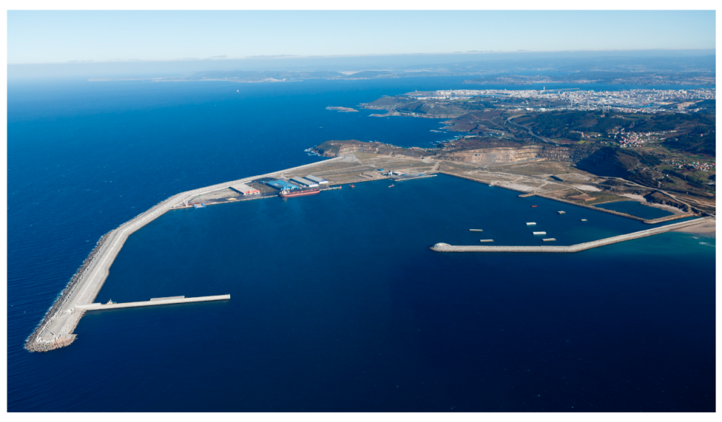
The data used to train and test the machine learning based models was collected at the Outer Port of Punta Langosteira (A Coruña), Spain (
Figure 1). Its geographical location entails that the meteorological conditions it is subject to are more severe than other inland ports. This port is located 10 km southeast of A Coruña, Spain, and is protected by a 3360 m long main breakwater and a 1320 m long spur breakwater. The current berthing line is 914 m long with an average depth of 22 m. The dock’s orientation is N62.7W and reaches a crest height of 6.5 m above the zero datum of the port. A set of bollards spaced 31 m apart with a load capacity of 200 T is situated 0.75 m from the dock. In addition, the vessel operations are streamlined by a double-fender system protected by a shield.
The section Materials and Methods explains the technical details of the dataset creation, which machine learning models were used, and how the models’ training and testing processes were carried out. The Results section presents the performance of the models.
2. Materials and Methods
The data used for training and testing the machine learning models was collected in five field campaigns, carried out in the outer port of Punta Langosteira (A Coruña), from October of 2015 until February of 2020. During these campaigns, we recorded the movement of 46 moored vessels for 1609 h total. We chose which vessels to monitor, from all available ships that operate in said port, so they reflect the typical fleet of the port. We also collected the environmental conditions (weather and sea state) the moored vessels were subject to during their port stay.
2.1. Dataset
The variables used to create the prediction models can be classified into meteorological conditions (weather conditions and sea state), ship characteristics, berthing location and ship movements. The models use the first two as inputs and output for the latter.
We gathered the weather conditions and sea state data using three measurement systems provided by the port technological infrastructure: a directional wave buoy, a weather station and a tide gauge.
The directional wave buoy is located 1.8 km off the main breakwater of the port (43°21′00′′ N 8°33′36′′ W). This buoy belongs to the Coastal Buoy Network of Puertos del Estado (REDCOS [
36]) and has the code 1239 in said network. Due to the sensibility of the buoy data to noise, the system provides its data aggregated in 1 h intervals. This quantization allows calculating some statistical parameters that reflect the sea state while mitigating the noise’s effects.
The weather station is located on the main port’s breakwater. It provides the data aggregated in 10 min intervals.
The tide gauge is also placed at the end of the main port’s breakwater. This tide gauge belongs to the Coastal Tide Gauges Network of Puertos del Estado (REDMAR [
37]) and has the code 3214 on said network. It provides the data in 1 min intervals.
From all the variables these data sources provide, we chose the variables also available in the port’s forecast system. This work’s objective is to create vessel movement models that, when used with weather and sea state forecasts as inputs, can predict future movements of a moored ship (as is further explained later in this section). In order to fulfill this objective, the models’ inputs regarding ocean-meteorological variables have to be those also available in the port’s forecast system. In summary, these are the meteorological variables we used as input variables to the model:
Hs (m): significant wave height, i.e., the mean of the highest third of the waves in a time-series of waves representing a certain sea state.
Tp (s): peak wave period, i.e., the period of the waves with the highest energy, extracted from the spectral analysis of the wave energy.
θm (deg): mean wave direction, i.e., the mean of all the individual wave directions in a time-series representing a certain sea state.
Ws (km/h): mean wind speed.
Wd (deg): mean wind direction.
H0 (m): sea level with respect to the zero of the port.
Hsm (m): significant wave height measured by the tide gauge, i.e., the mean of the highest third of the waves in a time-series of waves representing a certain sea state.
The buoy provides Hs, Tp and θm, the weather station provides Ws and Wd and the tide gauge provides H0 and Hsm.
The other category of variables used as inputs to the models is the ship characteristics and the berthing location. The ship’s geometric characteristics have high relevance in its dynamic behavior. Within the existing variables for the physical characteristics of a vessel, we used those whose acquisition was straightforward and always available. We also used the berthing zone as input to allow the model to capture the characteristics of the different locations of the port. The berthing zone would also allow creating a tool that loops over all available berthing zones and calculates the output of the models for each berthing zone, allowing the port operator to choose the best berthing location. The variables used are:
L (m): ship length.
B (m): ship breadth.
DWT (tonnes): deadweight tonnage, a measure of how much weight a ship can carry.
BZ: berthing zone. The port operator provides it. The port is divided into 12 berthing zones.
The port operator provided all the values for the previous variables.
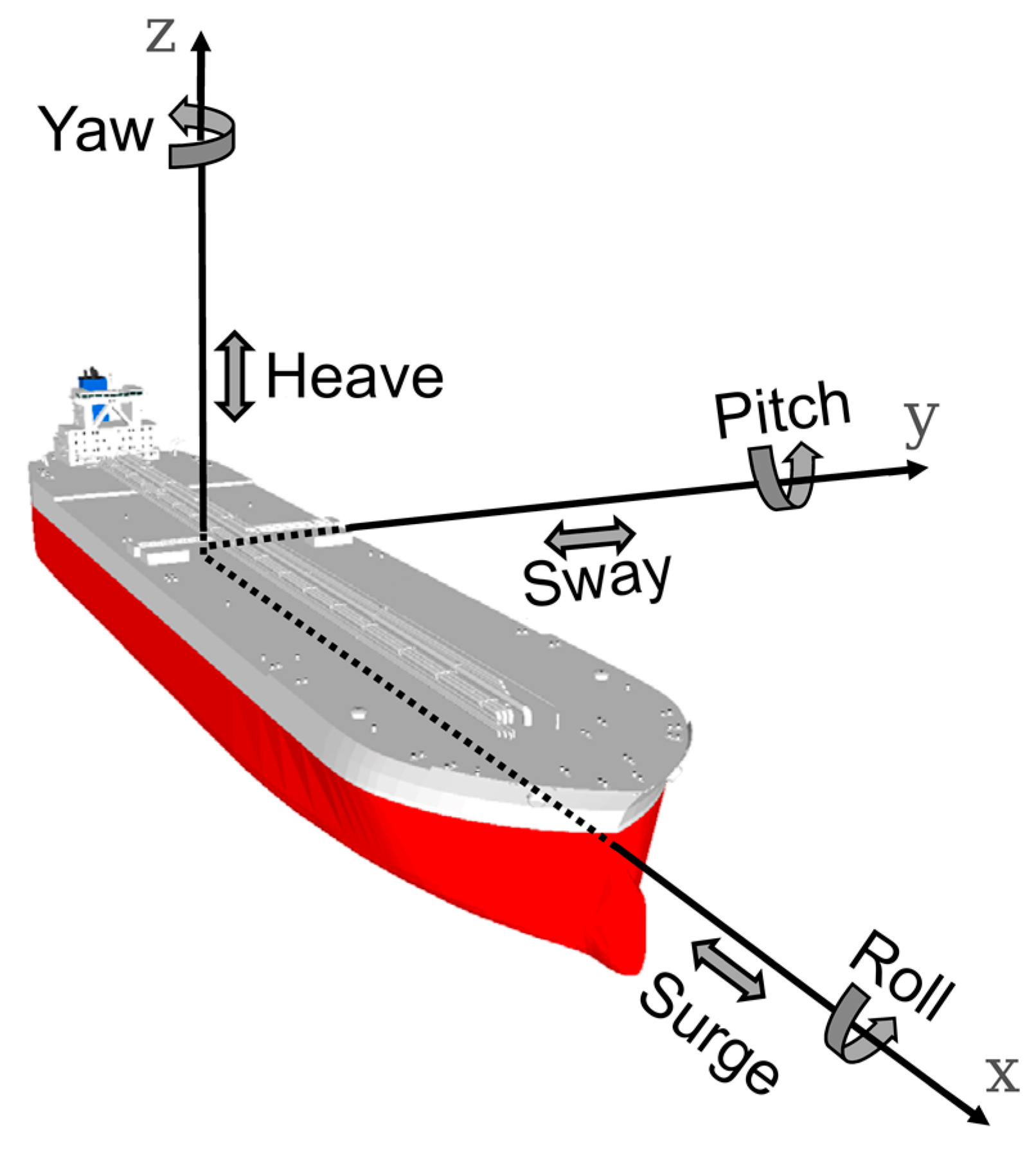
The last category of data, the ship’s movements, was used as outputs of the model. A moored vessel has six degrees of freedom (see
Figure 2): three displacements (surge, sway and heave) and three rotations (roll, pitch and yaw). The variables used for the vessel movement are:
Surge (m): linear longitudinal motion (bow-stern).
Sway (m): linear lateral motion (port-starboard).
Heave (m): linear vertical motion.
Roll (deg): tilting rotation of the vessel about its longitudinal axis (bow-stern).
Pitch (deg): up/down rotation of the vessel about its lateral axis (port-starboard).
Yaw (deg): turning rotation of the vessel about its vertical axis.
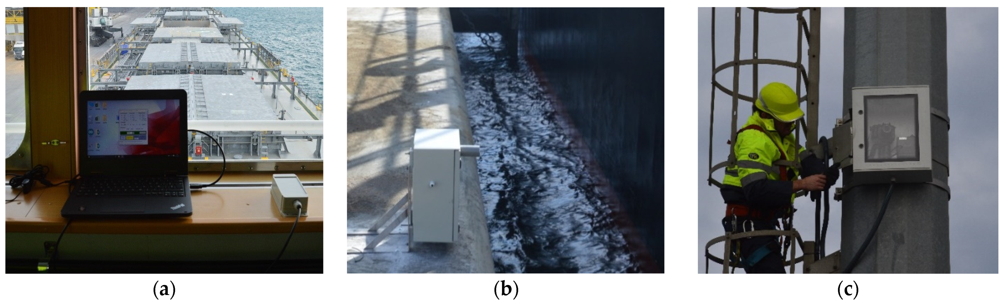
The methodology used to measure the ships’ movement, in its six degrees of freedom, is described in [
6,
7], where we used three complementary and fully synchronized measurement systems: an inertial measuring unit (IMU, a device that can measure and record the angular rate and specific gravity of the object to which it is attached to) (
Figure 3a), two laser distance meters (
Figure 3b) and two cameras (
Figure 3c). The combination of these devices allowed the recording of the movements at a minimum frequency of 1 Hz, which is enough to detect the movements of a moored vessel. The IMU provided the pitch and roll, two laser distance meters provided the sway and yaw and two cameras provided the surge and heave.
This work aimed to create vessel movement models that, when used with weather and sea state forecasts as inputs, can predict future movements of a moored ship. We created different machine learning models (artificial neural network, from now on referred to as ANN and gradient boosting with decision trees) and compared them to check which one provides the best results. In order to compare different machine learning models, we need them to use the same dataset so that we can compare them appropriately.
The first step in creating the dataset was joining the data provided by the several data sources (buoy, weather station, tide gauge, ship’s characteristics and ship’s movement monitoring). These data sources have a different frequency, so we had to aggregate the data to have the same frequency as the frequency of the data with the largest period, the sea state data, which is the same frequency as the data we will use as the models’ inputs in production. The variables that the forecast systems provided had a period of 1 h, so we needed to aggregate the rest of the variables and provide them with a 1 h period. When aggregating the data for the ship’s movements, we calculated the mean, maximum and significant (mean of the highest third) value for the amplitude of each movement for every hour.
A moored vessel may experience a maximum point motion much greater than its significant or average motion under the action of certain ocean-meteorological conditions. This value abandons the primary trend of the movement. It could occasionally be caused by external agents such as the waves generated by the passage of other ships or the punctual modification of the mooring lines’ tension to adapt them to the variations of the tidal range, making them difficult to predict. Therefore, we decided to select the significant value of each movement as the output of the models.
The wave parameters (significant wave height and peak period) were obtained similarly. These ship’s motion forcers are among those that most affect the motion of a moored ship. Therefore, using the same statistic for the inputs and outputs of the models could help the models to obtain a better relationship between these motion forcers and the ship’s movement. Moreover, other works used these values when studying moored vessels’ behavior [
14,
21], which demonstrates its feasibility as a motion descriptor.
Once we integrated and aggregated all data sources, we separated the dataset in two, creating a training and a testing dataset that we used to train and test the different models. Usually, the test dataset is created by randomly choosing data from the whole dataset but, had we had done this, the test results would have been inaccurate (overly optimistic). This is because the movement data of a ship for a specific stay is highly correlated, as it is temporal data: the ship’s movement for a given hour has a high correlation with the movement of the previous hour (they are close in the data distribution). Had we chosen random data from the whole dataset to create the testing dataset, the models would have obtained excellent results in testing since they would have been trained with data very similar to that used for testing (belonging to the same ship, similar environmental conditions and close temporal events). To avoid this, we created the test set by separating the data corresponding to two monitored vessels, so we did not train the models with data for those vessels. Thus, the test results will provide a more realistic estimation of how the models will perform in the production environment. In production, the port operators will use the models to predict a vessel’s movements in a real scenario (with vessels the model was not trained on).
The two selected vessels had characteristics in the same data distribution used for training: we chose a small general cargo ship (Dominica: 13,000 dwt and 127 m length) and a large bulk carrier (Fu Da: 71,500 dwt and 225 m length). We chose these vessels considering that they should provide enough information to conclude the performance of the models in a production environment, but without reducing too much the training dataset size. Thus, the testing dataset is around 10% of the whole dataset when using these two vessels.
To summarize, the dataset characteristics are the following:
We had two separate files for each movement: one for training and one for testing.
In each file, we had the previously explained variables: L, B, DWT, BZ, Hs, Tp, θm, Ws, Wd, H0 and Hsm and the corresponding mean movement, maximum movement and significant movement.
Each row in each file represents one hour of the ship’s movement (the data had a period of 1 h).
Table 1 shows the number of rows in each file.
The dataset is publicly available in [
38], where we provide a summarized description of the dataset and explain how to interpret it.
The dataset also stores variables not intended to be used as predictors, such as the ship’s name, the date of the ship’s stay and the ship’s type (general cargo or bulk carrier).
2.2. The Vessel Movement Predictors Creation
The vessel movement method used to create the dataset relies on the computer vision to measure several vessel movements [
6,
7]. A port’s infrastructure is not a controlled environment as a laboratory could be, so there are many technical limitations when using a camera to measure a vessel’s movement, occlusion being the most limiting. Furthermore, the vessels that operate in the outer port of Punta Langosteira are cargo ships. When a vessel is loading/unloading, there are many types of machinery such as cranes and trucks that occlude the camera field of view, making it impossible to measure the movements that rely on the computer vision. Given this limitation, not all movements are available for all the vessels at all times. To surpass this limitation and create precise prediction models, we decided to create one prediction model for each vessel movement, resulting in six models (one for each of the six degrees of freedom). Thus, each model uses the 11 input variables explained in the previous section and outputs one value for the corresponding movement.
For creating the prediction models, we chose two well-known and tested machine learning models for regression problems: gradient boosting [
39] and neural networks [
40].
Gradient boosting creates a prediction model via an ensemble of weak prediction models. In our case, the weak prediction models used are decision trees. When a decision tree is used as the weak learner, the boosting algorithm is usually called gradient boosted trees. Gradient boosted trees usually outperforms the random forest and have been used successfully to solve civil engineering problems [
41,
42].
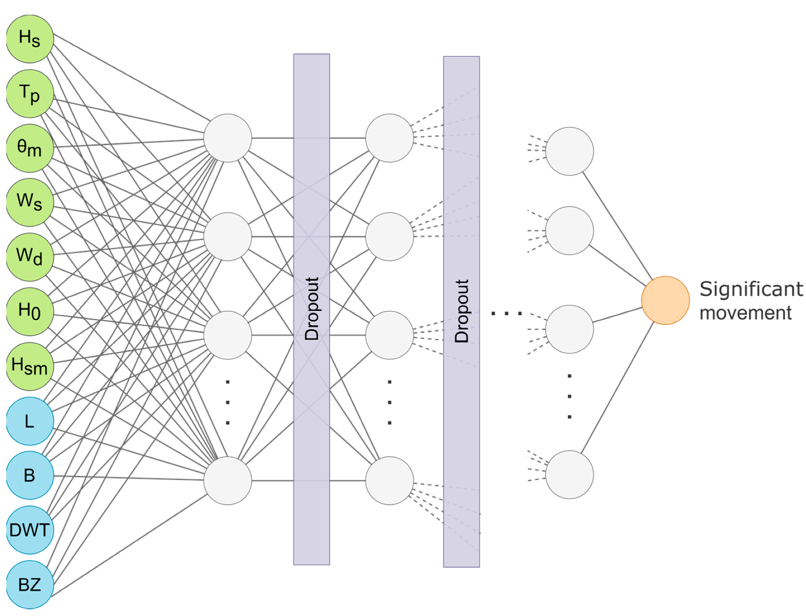
An artificial neural network is an interconnected group of nodes, where each interconnection has an associated weight. A node computes its output by applying a non-linear function to the sum of its inputs multiplied by the weight associated with each input. The variables used as inputs determine the ANN’s input nodes and they form the input layer. The variables used as outputs determine the ANN’s output nodes and they form the output layer. The layers of nodes between the input and output layers are called the hidden layer.
There is no proven methodology for choosing how many hidden layers and how many nodes per hidden layer are necessary to solve a given problem. Usually, one creates many different ANN architectures (with different layers and different nodes per layer), trains them and compares them using cross-validation. We followed this approach in this work.
The training process consisted of finding the appropriate weights for each interconnection, so the error for the training dataset was minimized (the output of the ANN was as close as possible to the desired output when we gave the corresponding input data to the ANN).
Figure 4 shows a representation of the overall architecture of the ANNs created in this work. The hidden layers and the dropout ratio varied for each of the six models obtained, but the overall structure remained the same.
The objective of an ANN is to approximate a function 𝑓 that provides the desired output given the input. While a sufficiently complex ANN can approximate any function 𝑓, an ANN is a black box. Analyzing the ANN structure will not give insights into the function being approximated: there is no simple link between the weights and the function being approximated. Despite this lack of interpretability, ANN has successfully solved coastal engineering problems [
30,
31,
32] and other subdisciplines of civil engineering [
33,
34,
35].
We trained and tested both types of models using the same training and testing dataset to check, which one gives the best results. The training process, in each case, consisted of creating multiple models with different hyperparameters and comparing them using 10-fold cross-validation. Once the best model, the one that performed the best using cross-validation, was selected, we assessed its performance by using the testing datasets. We explain the overall process in Algorithm 1.
| Algorithm 1: Pseudocode for the iterative grid-based training process algorithm. |
do
manually define grid of model hyperparameters
for each grid cell (model) do
for each resampling iteration do
hold-out specific samples
fit model on the remainder
predict the hold-out samples
end
calculate average performance across hold-out predictions
end
determine best hyperparameter
fit final model (best hyperparameter) to all training data
while error >= ε
evaluate final model performance in test set |
The hyperparameters’ value for a specific model is chosen from a grid created as the outer product of all the values manually specified used for each hyperparameter.
The hyperparameters we need to define and the values used for the gradient boosting models are the following:
N.trees: this hyperparameter represents the number of gradient boosting iterations (number of trees). Increasing N reduces the error on the training set, but setting it too high may lead to overfitting. We tried the values 1000, 2000, 3250, 5000, 7000, 8500, 10,000 and 15,000 for this hyperparameter.
Shrinkage: this hyperparameter represents the learning rate. We tried the values 0.1, 0.01 and 0.001 for this hyperparameter.
Interaction.depth: this parameter represents the depth of each tree. We tried the values 1, 5 and 9 for this hyperparameter.
N.minobsinnode: this hyperparameter represents the minimum number of observations required in the tree terminal nodes (leaves). We tried the values 3, 5 and 10 for this hyperparameter.
ANNs are a more powerful model than gradient boosting, but they require more data and time to train and there are more hyperparameters we need to tune. The hyperparameters we need to define and the values we used for the ANN models are the following:
Network architecture: we tested networks with 1, 2, 3 and 4 layers. We tried with 8, 16, 32, 64, 128 and 256 neurons per layer in each case. The layers were fully connected in all cases. Although the largest networks could seem too complex for the problem at hand, we used them because we planned to use dropout regularization and one is likely to get better performance when dropout is used on a larger network (dropout is going to prune the network resulting in a smaller network). Using a small network with dropout could result in a model too simple to be a good predictor.
Weights (kernel) initialization: we used several weights initialization, both the uniform and the normal variations, for random, He [
43] and Glorot (a.k.a. Xavier) [
44] initializations.
Optimizer: we used 3 different optimizers, stochastic gradient descent (SGD) [
45], RMSprop [
46] and Adam [
47].
Training iterations: we tested the optimizer with 2000, 5000, 7000 and 10,000 iterations. The results did not improve from 5000 iterations up, so we chose 5000 for all the following iterations.
Activation function: we tested several activation functions for the neurons in the hidden layers: ReLU, SeLu, eLu and tanh.
Training iterations: we tested each optimizer with 500, 1000, 2000, 2500 and 5000 training iterations.
Regularization: we used dropout regularization [
48], with one dropout layer for each hidden layer (except the output layer). We tested several dropout rates: none, 0.0625, 0.125, 0.25 and 0.375, where none indicates that no dropout was used.
Learning rate: we tested several values for the learning rate: [0.0001, 0.001, 0.01, 0.1]. Although 0.01 and 0.1 are usually considered too large learning rates, large values are suggested in the original dropout paper [
48].
Once we trained all the models using cross-validation (as described in Algorithm 1), we selected the best 12 models, i.e., we had two models for each of the six degrees of freedom of a vessel movement. One is an ANN model and another a gradient boosting model. We tested both models with the test data for the corresponding movement to select the best one for each movement. We present all the training and testing results in the next section.
3. Results and Discussion
A machine learning model was fully specified by its inputs, outputs and hyperparameters. The hyperparameters for the best gradient boosting model for each movement, obtained using the method previously described, are shown in
Table 2.
We can see in
Table 2 that in all movements, but surge, the best models were the ones with more complexity in terms of tree depth, but only the models for surge and heave required to create a higher number of trees to provide the best results. None of the models required more than 8500 trees, although the values 10,000 and 15,000 were also used.
We show the hyperparameters for the best ANN based models for each movement in
Table 3.
We can see in
Table 3 that in every case, using ReLU units provided the best results. Additionally, in every case, the He uniform initialization gave the best results. These results were consistent with the state-of-the-art recommendation of using He uniform initialization when using ReLU units.
We can see that the results we show in
Table 2 and
Table 3 for the model of the surge movement and the model of the heave movement were consistent: they required the most complex models, both in the ANN and the gradient boosting cases. The gradient boosting models required more trees for modeling the movement, and the ANN models required a larger network. This need for more complex models was caused by the situation previously explained: we had less data for these movements, as they rely on computer vision techniques to measure them.
Table 4 shows the comparison between the training error, in terms of the root mean squared error (RMSE), of both the ANN and the gradient boosting model for each movement. The RMSE alone does not measure how good a model is if we do not compare it with the range of the movement that the model is predicting. We considered that a model has good performance if its RMSE is less than or equal to 10% of the range for the movement it is predicting. We show this limit as the “0.1 range” value in
Table 4 to quickly compare the RMSE with this limit. We can see that all models for every movement had a lower RMSE than 10% of the movement range, so we considered that they achieved the goal we initially set.
Table 4 also shows the coefficient of determination (R
2) that each model achieved in the training dataset. We can see that the ANN models achieved a higher R
2 than the gradient boosting models for every movement, being higher than 0.95 in every case. The worst R
2 for a gradient boosting model was 0.86, achieved in the case of the surge movement. This result was consistent with having less data for this movement, as previously explained.
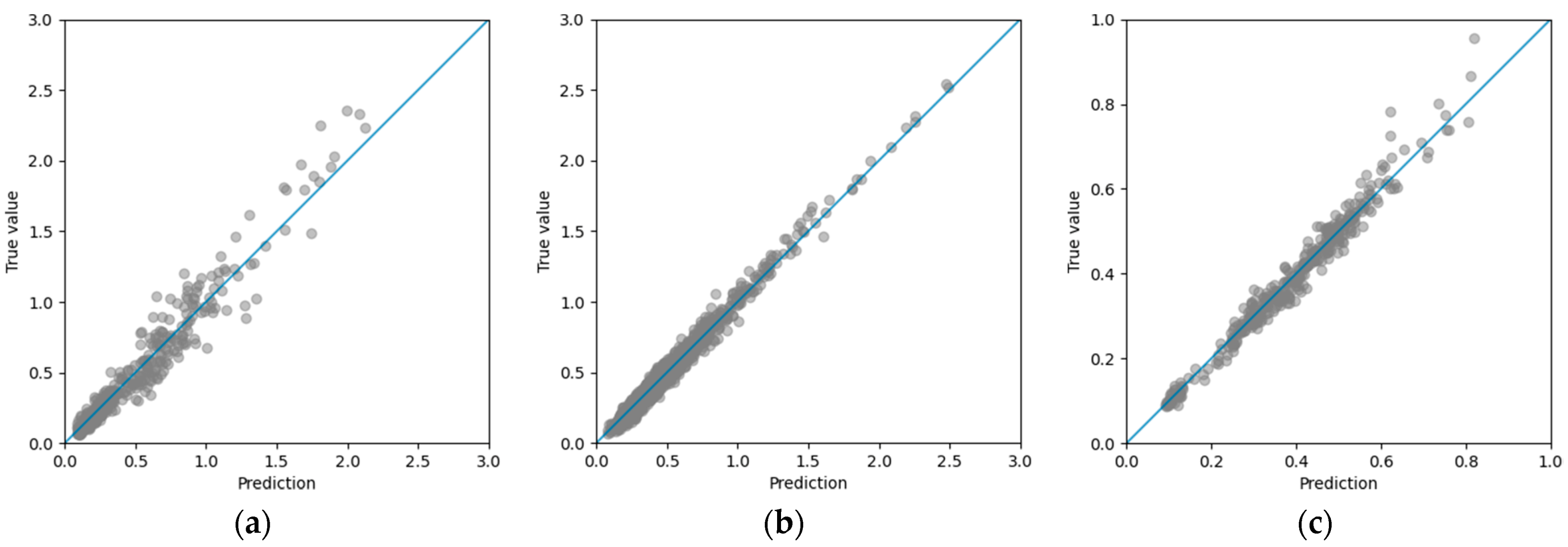
To analyze where the models failed the most, we could plot the true values for each movement against the corresponding model predictions. A perfect prediction would fall on the line y = x.
Figure 5 shows the plots of the true outputs versus the predictions of the gradient boosting models for the training dataset. In these plots, we show the y = x line in blue.
We can see in
Figure 5 that the surge prediction model error increased as the amplitude of the motion increased, and the error for the heave movement was primarily due to a worse prediction of the larger movements. We can also see that the error for the roll movement was committed during all the movement ranges.
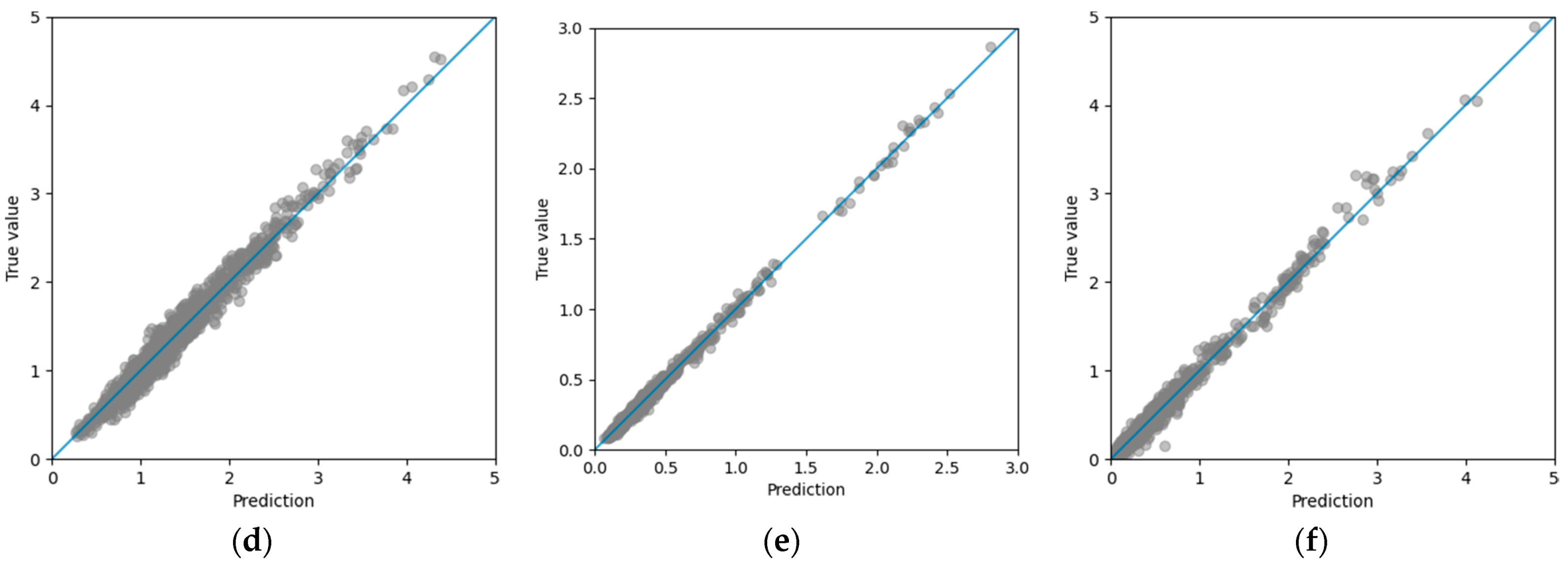
Figure 6 shows the plots of the true outputs versus the predictions of the ANN models for the training dataset. In these plots, we show the y = x line in blue.
We can see in
Figure 6 that the predictions were overall good. The model for the sway movements underestimated the amplitudes of the larger movements a bit. The model for the heave movement underestimated the shorter movements and overestimated the larger movements. In the model for the pitch movement, the mid and large movements predictions were more dispersed and the same happened for the larger movements in the yaw model.
After the training phase, where we obtained the best models for each movement, both using the ANN and the gradient boosting models, we tested them using the testing dataset. The results, in terms of the RMSE obtained for each movement and type of model are shown in
Table 5. We also show the “0.1 range” value to quickly compare the testing RMSE with this limit.
In testing, we also considered that a model had good performance if its RMSE was less than or equal to 10% of the range for the movement it was predicting. We can see in
Table 5 that all ANN models but the one for heave and roll were below the 10% error margin. In the gradient boosting models case, all the models but the one for surge and roll were below the limit and the model for the heave movement was right on the limit. As previously explained, we had less training data for the heave and surge movements, so we could expect that the corresponding model predictions in the testing dataset were in the error limit or above it.
The two models for the roll motion showed the least satisfactory results, probably because the ships used were out of range for this motion. The roll movement of a vessel shows a greater variability for similar ocean-meteorological conditions than the other movements, increasing the difficulty for a model to represent the relationship between inputs and outputs when not enough data is available.
4. Conclusions
In this work, we developed prediction models for the movement of a moored ship using data from 46 ships obtained between October 2015 and February 2020 in the outer port of Punta Langosteira, Spain. Using the gathered data, we created prediction models based on two well-known machine learning models that have been used successfully to solve civil engineering problems: gradient boosted trees [
21,
22] and artificial neural networks [
9,
10,
11,
12,
13,
14].
We set the limit for deciding if the models performed satisfactorily as having an RMSE lower than 10% of the corresponding movement range.
The best models achieved satisfactory results in the training dataset, having an RMSE lower than the limit in every case. The coefficient of determination (R2) was 0.99, 0.99, 0.95, 0.99, 0.98 and 0.98 for the surge, sway, heave, roll, pitch and yaw movements, respectively, for the best models. These R2 values were achieved by the ANN models, which showed to be more powerful than the gradient boosting models (they had lower RMSE and higher R2) as they proved to have less bias. The counterpart is that ANN requires tuning more hyperparameters, more time to train and more data than the gradient boosting models to achieve better results.
The surge, sway, pitch and yaw models performed satisfactorily in the testing dataset, having an RMSE lower than 10% of the corresponding movement range. Although we created the heave and surge movements models, we did not have enough data to feel confident about the corresponding models’ performance. However, the ANN heave model performed satisfactorily both in the training and testing.
In any case, increasing the volume of data available for training the models will improve their performance, especially in the ranges of motion where we did not have enough data to be confident in the model predictions. In addition, increasing the dataset is another way to avoid overfitting, so the need for regularization will be reduced and the training process could be accelerated.
The main limitations of the approach used in this work, and in any machine learning-based solution, were the lack of (good) data and the interpretability.
Many machine learning models require large amounts of data to provide useful results. For instance, in the case of neural networks, the larger the model’s architecture, the more data we need to use for training it to produce good results. Some techniques, such as data augmentation, are useful to some extent, but the preferred solution is always obtaining more data, when possible.
In future works, we plan to increase the dataset via an intensive monitoring campaign focusing on the surge and heave movements to improve the models results. Unfortunately, in the last two campaigns (2020 and 2021), due to the situation generated by COVID-19, access to the interior of moored ships in the outer port of Punta Langosteira was prohibited. Hence, we could not use the IMU to record the ships’ movements, so the roll and pitch dataset did not increase as much as intended.
Another data-related limitation is when data with potential bias finds its way into the data set or the models (via the training process). This circumstance could lead to situations where models that are seemingly performing well may actually be picking up noise in the data. This problem is more prominent in data with high variability than in slow-changing or bounded data, i.e., in data with high variability, we cannot accurately detect when there is noise in the data (in slow-changing data or data with values restricted to a small range, the noise is more evident).
The ideal solution to this problem is collecting data from multiple sources. Having multiple sources limits the effect that bias has on the models, resulting in higher quality models. To mitigate this problem, in future works, we plan to study and search for theoretical new variables that could improve predicting movements with high variability, such as the roll movement.
Interpretability is one of the primary problems with machine learning, as any user related problem in computer science.
The machine learning models created in this work are intended to replace traditional statistical methods used in port management tools. These traditional models are interpretable, a characteristic that port operators are accustomed to.
Using machine learning models we cannot explain to port operators how and why the model came to the decision it did. The only tool a machine learning practitioner has in this situation is to convince through results, i.e., the models need to prove that they are superior to traditional statistical methods by providing more accurate predictions than traditional models.
During the development of this work, and after obtaining the results, we maintained several meetings with the A Coruña port authority and the port operators. After reviewing the result obtained in this work, they are convinced that machine learning methods provide better results than traditional methods, despite the lack of interpretability. They intend to use the models created in this work in their decision-making pipeline.
To facilitate this, we intend to create a decision-aiding tool that uses the models created in this work. Currently, port operators do not have a tool such as this one that allows predicting whether a ship will exceed the recommended limits for the cargo ship movements during loading and unloading operations (determined by the Spanish Port Authority). Instead, they take a conservative approach, sometimes stopping the operations unnecessarily. Having this tool will improve the decision-making pipeline and optimize the ship’s operations.
To summarize all future works, after gathering more data and new variables, we intend to optimize the models, retrain them and incorporate them in a web tool that will allow easy access to the model predictions to the port operators. The tool will use forecast data for the weather conditions and sea state as inputs for the models (and the ship characteristics and berthing location) to predict the ship movements several days in advance. These predictions can aid in deciding the best location for the operation and in deciding when to stop the ship operations more precisely, thus minimizing the economic impact the hydrodynamic phenomena have due to cargo ships being unable to operate.
Author Contributions
Conceptualization, J.R., E.P., A.F., A.A., J.S. and A.G.; methodology, J.R., A.A., A.F. and J.S.; software, A.A. and H.C.; validation, A.A., A.F. and H.C.; formal analysis, E.P., A.F., A.A. and J.S.; investigation, A.A., A.F., H.C. and R.C.; resources, J.R., E.P. and A.G.; data curation, A.A., A.F., H.C. and R.C.; writing—original draft preparation, A.A. and A.F.; writing—review and editing, A.A. and A.F.; visualization, A.F., E.P., J.S. and A.G.; supervision, J.R. and E.P.; project administration, E.P. and J.R.; funding acquisition, A.F., E.P. and J.R. All authors have read and agreed to the published version of the manuscript.
Funding
This research was funded by the Spanish Ministry of Economy, Industry, and Competitiveness, R&D National Plan, within the project BIA2017-86738-R, the FPI predoctoral grant from the Spanish Ministry of Science, Innovation, and Universities (PRE2018-083777) and the Spanish Ministry of Science and Innovation, Retos Call, within the project PID2020-112794RB-I00.
Institutional Review Board Statement
Not applicable.
Informed Consent Statement
Not applicable.
Data Availability Statement
Acknowledgments
The authors wish to thank the staff of Port Authority of A Coruña. Moreover, the authors are grateful to the owners and crew of the vessels for their collaboration on board.
Conflicts of Interest
The authors declare no conflict of interest.
References
- Puertos del Estado (Spanish Port System). Available online: http://www.puertos.es/en-us (accessed on 28 June 2021).
- Mooring of Ships to Piers and Wharves; Coasts, Oceans, Ports and Rivers Institute (American Society of Civil Engineers); Gaythwaite, J. (Eds.) ASCE manuals and reports on engineering practice; American Society of Civil Engineers: Reston, VA, USA, 2014; ISBN 978-0-7844-1355-5. [Google Scholar]
- PIANC General Secretariat; Maritime Navigation Commission; World Association for Waterborne Transport Infrastructure. Criteria for the (Un) Loading of Container Vessels; PIANC Secrétariat Général: Bruxelles, Belgique, 2012; ISBN 978-2-87223-195-9. [Google Scholar]
- Criteria for Movements of Moored Ships in Harbours: A Practical Guide; Supplement to Bulletin; Permanent International Association of Navigation Congresses: Bruxelles, Belgique, 1995; ISBN 978-2-87223-070-9.
- Llorca, J.; González Herrero, J.M.; Ametller, S.; Ente Público Puertos del Estado (España). ROM 2.0-11: Recomendaciones Para el Proyecto y Ejecución en Obras de Atraque y Amarre; Puertos del Estado: Madrid, Spain, 2012; ISBN 978-84-88975-78-2.
- Figuero, A.; Rodriguez, A.; Sande, J.; Peña, E.; Rabuñal, J.R. Dynamical Study of a Moored Vessel Using Computer Vision. J. Mar. Sci. Technol. 2018, 26, 240–250. [Google Scholar] [CrossRef]
- Figuero, A.; Rodriguez, A.; Sande, J.; Peña, E.; Rabuñal, J.R. Field Measurements of Angular Motions of a Vessel at Berth: Inertial Device Application. J. Control. Eng. Appl. Inform. 2018, 20, 79–88. [Google Scholar]
- Baker, S.; Frank, G.; Cornett, A.; Williamson, D.; Kingery, D. Physical Modelling and Design Optimizations for a New Container Terminal at the Port of Moin, Costa Rica. In Ports 2016; American Society of Civil Engineers: New Orleans, LA, USA, 2016; pp. 560–569. [Google Scholar]
- Cornett, A.; Wijdeven, B.; Boeijinga, J.; Ostrovsky, O. 3-D Physical Model Studies of Wave Agitation and Moored Ship Motions at Ashdod Port. In Proceedings of the 8th International Conference on Coastal and Port Engineering in Developing Countries, Chennai, India, 20–24 February 2012. [Google Scholar]
- Jorge Rosa-Santos, P.; Taveira-Pinto, F. Experimental Study of Solutions to Reduce Downtime Problems in Ocean Facing Ports: The Port of Leixões, Portugal, Case Study. J. Appl. Water Eng. Res. 2013, 1, 80–90. [Google Scholar] [CrossRef]
- Rosa-Santos, P.; Taveira-Pinto, F.; Veloso-Gomes, F. Experimental Evaluation of the Tension Mooring Effect on the Response of Moored Ships. Coast. Eng. 2014, 85, 60–71. [Google Scholar] [CrossRef]
- Kumar, P.; Batra, G.; Kim, K.I. A Moored Ship Motion Analysis in Realistic Pohang New Harbor and Modified PNH. In Modern Mathematical Methods and High Performance Computing in Science and Technology; Singh, V.K., Srivastava, H.M., Venturino, E., Resch, M., Gupta, V., Eds.; Springer Proceedings in Mathematics & Statistics; Springer: Singapore, 2016; Volume 171, pp. 207–214. ISBN 978-981-10-1453-6. [Google Scholar]
- Howle, M.; Bont, J.D.; Molen, W.; Lem, J.; Ligteringen, H.; Mühlenstein, D. Calculations of the Motions of a Ship Moored with MoorMaster Units. In Proceedings of the 32nd PIANC International Navigation Congress, Liverpool, UK, 10–14 May; The World Association for Waterborne Transport Infrastructure (PIANC): Liverpool, UK, 2010; pp. 622–635. [Google Scholar]
- Van der Molen, W.; Scott, D.; Taylor, D.; Elliott, T. Improvement of Mooring Configurations in Geraldton Harbour. J. Mar. Sci. Eng. 2016, 4, 3. [Google Scholar] [CrossRef] [Green Version]
- Kwak, M. Numerical Simulation of Moored Ship Motion Considering Harbor Resonance. In Handbook of Coastal and Ocean Engineering; WORLD SCIENTIFIC: Singapore, 2018; pp. 1081–1110. ISBN 978-981-320-401-0. [Google Scholar]
- Cummins, W.E. The Impulse Response Function and Ship Motions; Navy Dept., David Taylor Model Basin: Carderock, MD, USA, 1962.
- Van der Molen, W.; Ligteringen, H.; Van der Lem, J.C.; De Waal, J.C.M. Behavior of a Moored LNG Ship in Swell Waves. J. Waterw. Port Coast. Ocean. Eng. 2003, 129, 15–21. [Google Scholar] [CrossRef]
- Van Deyzen, A.F.J.; Beimers, P.B.; Van der Lem, J.C.; Messiter, D.; De Bont, J.A.M. To Improve the Efficiency of Ports Exposed to Swell. In Proceedings of the Australasian Coasts & Ports Conference 2015: 22nd Australasian Coastal and Ocean Engineering Conference and the 15th Australasian Port and Harbour Conference, Auckland, New Zealand, 15–18 September 2015; pp. 919–926. [Google Scholar]
- Trejo, I.; Pérez, J.; Guerra, A.; Iribarren, J.R.; Gómez, J.; Sopelana, J.; Peña González, E. Onsite Measurement of Moored Ships Behaviour (RTK GPS), Waves and Long Waves in the Outer Port of A Coruña (Spain). In Proceedings of the 33rd PIANC World Congress, San Francisco, CA, USA, 1–5 June 2014. [Google Scholar]
- Van Zwijnsvoorde, T.; Vantorre, M.; Ides, S. Container Ships Moored at the Port of Antwerp: Modelling Response to Passing Vessels. In Proceedings of the 34th PIANC World Congress, Panama City, Panama, 7–11 May 2018; pp. 1–18. [Google Scholar]
- López, M.; Iglesias, G. Long Wave Effects on a Vessel at Berth. Appl. Ocean. Res. 2014, 47, 63–72. [Google Scholar] [CrossRef]
- Jensen, O.J.; Viggosson, G.; Thomsen, J.; Bjordal, S.; Lundgren, J. Criteria for Ship Movements in Harbours. In Proceedings of the Coastal Engineering 1990, Delft, The Netherlands, 20 May 1990; American Society of Civil Engineers: Delft, The Netherlands, 1991; pp. 3074–3087. [Google Scholar]
- Figuero, A.; Sande, J.; Peña, E.; Alvarellos, A.; Rabuñal, J.R.; Maciñeira, E. Operational Thresholds of Moored Ships at the Oil Terminal of Inner Port of A Coruña (Spain). Ocean. Eng. 2019, 172, 599–613. [Google Scholar] [CrossRef]
- Hiraishi, T.; Atsumi, Y.; Kunita, A.; Sekiguchi, S.; Kawaguchi, T. Observation of Long Period Wave and Ship Motion in Tomakomai-Port. In Proceedings of the 7th International Offshore and Polar Engineering Conference, Honolulu, HI, USA, 25–30 May 1997. [Google Scholar]
- Uzaki, K.; Matsunaga, N.; Nishii, Y.; Ikehata, Y. Cause and Countermeasure of Long-Period Oscillations of Moored Ships and the Quantification of Surge and Heave Amplitudes. Ocean. Eng. 2010, 37, 155–163. [Google Scholar] [CrossRef]
- Sakakibara, S.; Saito, K.; Kubo, M.; Shiraishi, S.; Nagai, T.; Shimanoe, S. A Study on Long-Period Moored Ship Motions in a Harbor Induced by a Resonant Large Roll Motion during Long Waves. J. Jpn. Inst. Navig. 2001, 104, 187–196. [Google Scholar] [CrossRef]
- Kwak, M.; Pyun, C. Computer Simulation of Moored Ship Motion Considering Harbor Resonance in Pohang New Harbor. In Ports 2013; American Society of Civil Engineers: Seattle, WA, USA, 2013; pp. 1415–1424. [Google Scholar]
- MarineTraffic: Global Ship Tracking Intelligence|AIS Marine Traffic. Available online: https://www.marinetraffic.com/en/ais/home/centerx:-12.1/centery:25.0/zoom:4 (accessed on 28 June 2021).
- Free AIS Ship Tracking of Marine Traffic-VesselFinder. Available online: https://www.vesselfinder.com/ (accessed on 28 June 2021).
- Yin, J.; Zou, Z.; Xu, F. On-Line Prediction of Ship Roll Motion during Maneuvering Using Sequential Learning RBF Neuralnetworks. Ocean. Eng. 2013, 61, 139–147. [Google Scholar] [CrossRef]
- Kumar, N.K.; Savitha, R.; Mamun, A.A. Regional Ocean Wave Height Prediction Using Sequential Learning Neural Networks. Ocean. Eng. 2017, 129, 605–612. [Google Scholar] [CrossRef]
- Rigos, A.; Tsekouras, G.E.; Vousdoukas, M.I.; Chatzipavlis, A.; Velegrakis, A.F. A Chebyshev Polynomial Radial Basis Function Neural Network for Automated Shoreline Extraction from Coastal Imagery. Comput. Aided Eng. 2016, 23, 141–160. [Google Scholar] [CrossRef] [Green Version]
- Cha, Y.-J.; Choi, W.; Büyüköztürk, O. Deep Learning-Based Crack Damage Detection Using Convolutional Neural Networks. Comput. Aided Civ. Infrastruct. Eng. 2017, 32, 361–378. [Google Scholar] [CrossRef]
- Lin, Y.; Nie, Z.; Ma, H. Structural Damage Detection with Automatic Feature-Extraction through Deep Learning. Comput. Aided Civ. Infrastruct. Eng. 2017, 32, 1025–1046. [Google Scholar] [CrossRef]
- Xue, Y.; Li, Y. A Fast Detection Method via Region-Based Fully Convolutional Neural Networks for Shield Tunnel Lining Defects. Comput. Aided Civ. Infrastruct. Eng. 2018, 33, 638–654. [Google Scholar] [CrossRef]
- Red Costera de Boyas de Oleaje de Puertos Del Estado (REDCOS). Available online: https://bancodatos.puertos.es/BD/informes/INT_1.pdf (accessed on 28 June 2021).
- Red de Medida Del Nivel Del Mar y Agitación de Puertos Del Estado (REDMAR). Available online: https://bancodatos.puertos.es/BD/informes/INT_3.pdf (accessed on 28 June 2021).
- Alvarellos, A. aalvarell/ship-movement-dataset: Outer Port of Punta Langosteira ship movement dataset (Version v1.0.0). Github 2021. [Google Scholar] [CrossRef]
- Hastie, T.; Tibshirani, R.; Friedman, J. Neural Networks. In The Elements of Statistical Learning: Data Mining, Inference, and Prediction; Hastie, T., Tibshirani, R., Friedman, J., Eds.; Springer Series in Statistics; Springer: New York, NY, USA, 2009; pp. 389–416. ISBN 978-0-387-84858-7. [Google Scholar]
- Hastie, T.; Tibshirani, R.; Friedman, J. Boosting and Additive Trees. In The Elements of Statistical Learning: Data Mining, Inference, and Prediction; Hastie, T., Tibshirani, R., Friedman, J., Eds.; Springer Series in Statistics; Springer: New York, NY, USA, 2009; pp. 337–387. ISBN 978-0-387-84858-7. [Google Scholar]
- Piryonesi, S.M.; El-Diraby, T.E. Data Analytics in Asset Management: Cost-Effective Prediction of the Pavement Condition Index. J. Infrastruct. Syst. 2020, 26, 04019036. [Google Scholar] [CrossRef]
- Madeh Piryonesi, S.; El-Diraby, T.E. Using Machine Learning to Examine Impact of Type of Performance Indicator on Flexible Pavement Deterioration Modeling. J. Infrastruct. Syst. 2021, 27, 04021005. [Google Scholar] [CrossRef]
- He, K.; Zhang, X.; Ren, S.; Sun, J. Delving Deep into Rectifiers: Surpassing Human-Level Performance on ImageNet Classification. arXiv 2015, arXiv:1502.01852. [Google Scholar]
- Glorot, X.; Bengio, Y. Understanding the Difficulty of Training Deep Feedforward Neural Networks. In Proceedings of the Thirteenth International Conference on Artificial Intelligence and Statistics, Sardinia, Italy, 13–15 May 2010; Volume 9, pp. 249–256. [Google Scholar]
- Kiefer, J.; Wolfowitz, J. Stochastic Estimation of the Maximum of a Regression Function. Ann. Math. Statist. 1952, 23, 462–466. [Google Scholar] [CrossRef]
- Hinton, G.E. RMSPROP. 2014. Available online: http://www.cs.toronto.edu/~tijmen/csc321/slides/lecture_slides_lec6.pdf (accessed on 28 June 2021).
- Kingma, D.P.; Ba, J. Adam: A Method for Stochastic Optimization. arXiv 2017, arXiv:1412.6980. [Google Scholar]
- Srivastava, N.; Hinton, G.; Krizhevsky, A.; Sutskever, I.; Salakhutdinov, R. Dropout: A Simple Way to Prevent Neural Networks from Overfitting. J. Mach. Learn. Res. 2014, 15, 1929–1958. [Google Scholar]
| Publisher’s Note: MDPI stays neutral with regard to jurisdictional claims in published maps and institutional affiliations. |
© 2021 by the authors. Licensee MDPI, Basel, Switzerland. This article is an open access article distributed under the terms and conditions of the Creative Commons Attribution (CC BY) license (https://creativecommons.org/licenses/by/4.0/).


 ,
, 


