
Combined Longshore and Cross-Shore Modeling for Low-Energy Embayed Sandy Beaches

 , , , and
Abstract
:1. Introduction
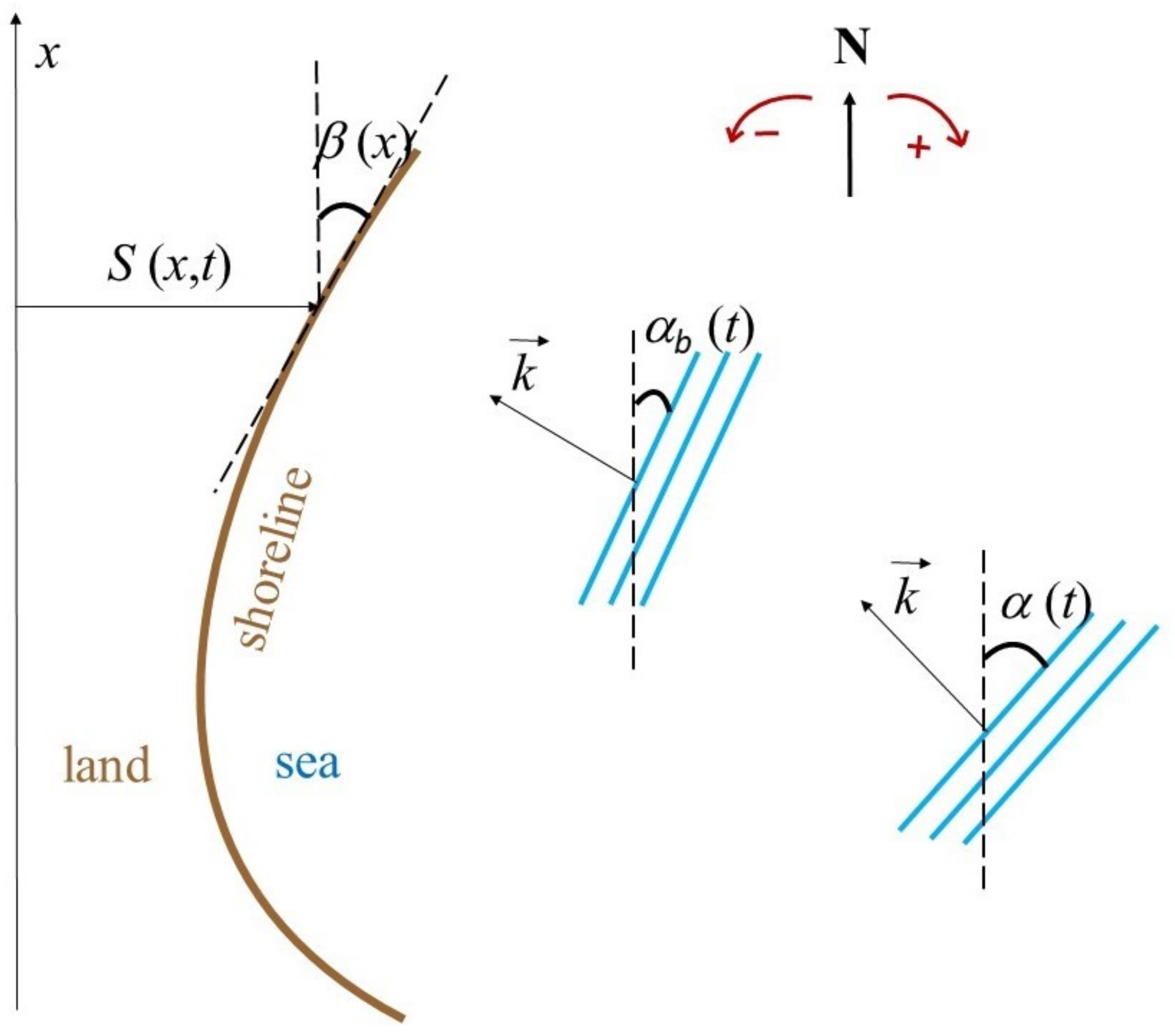
2. Methods
3. Study Site
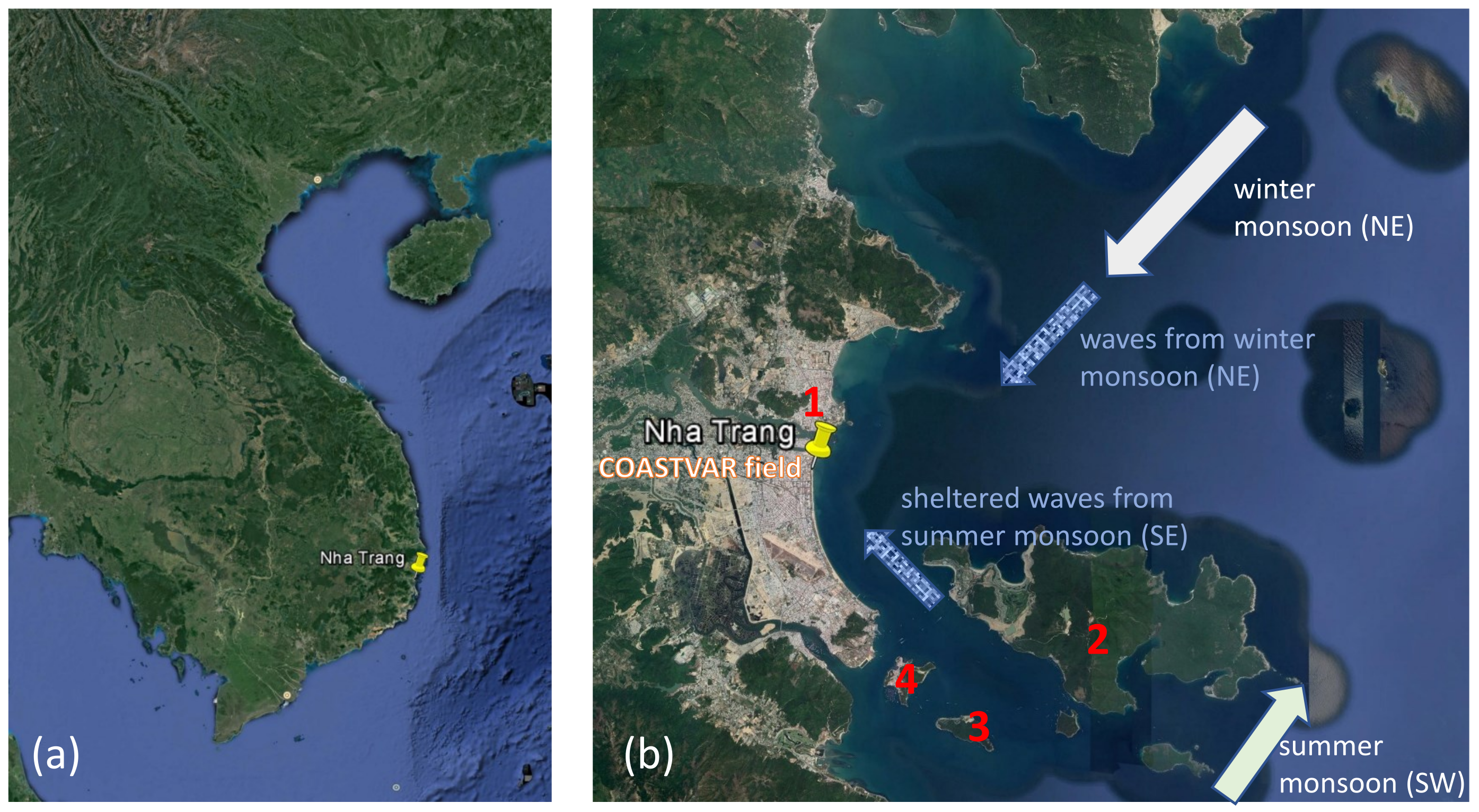
3.1. Site Description
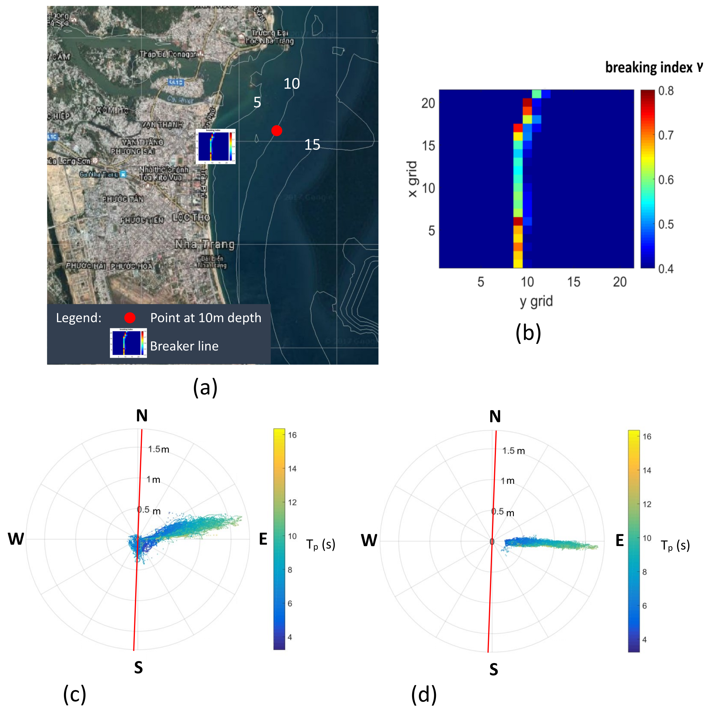
3.2. Waves
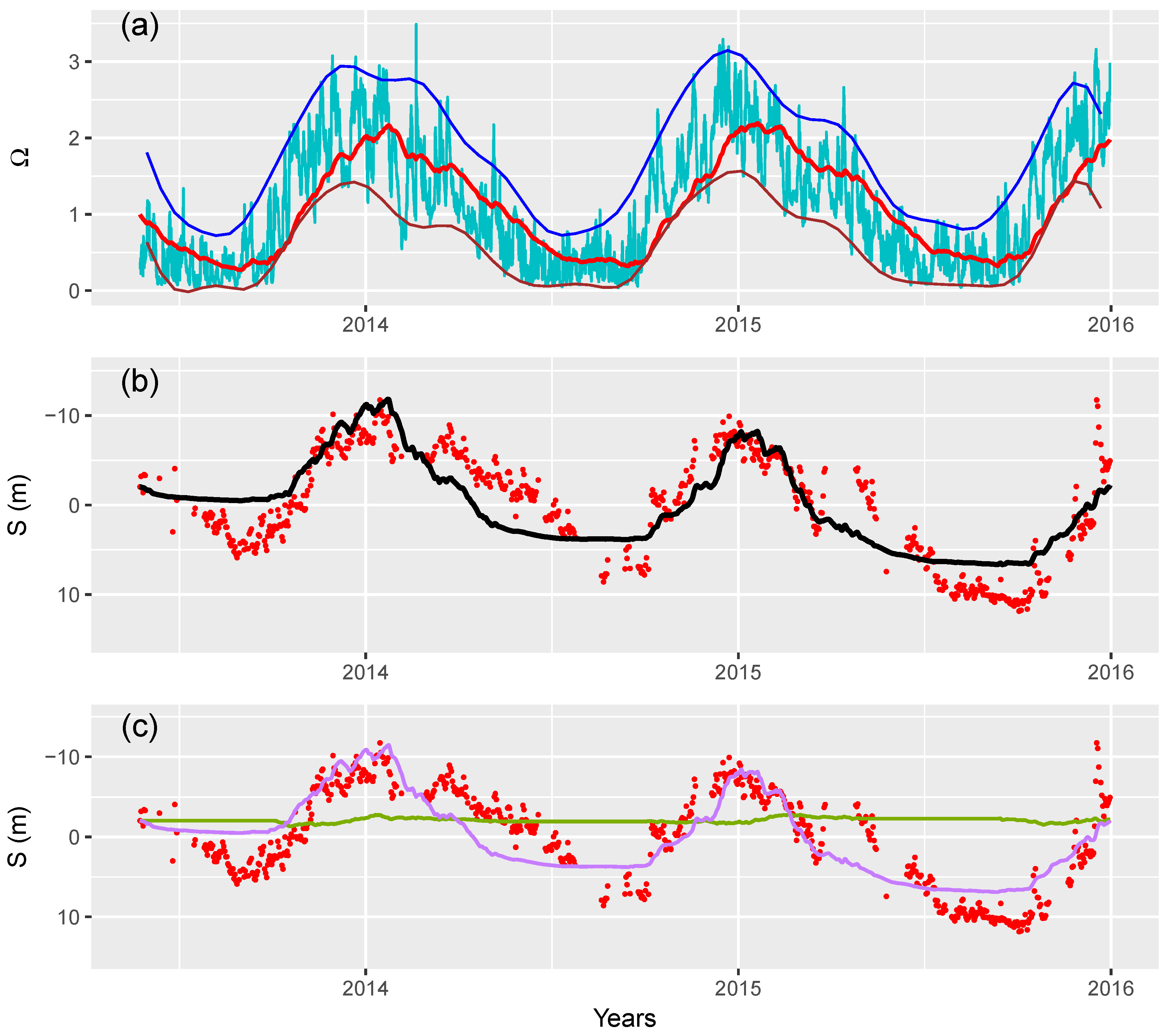
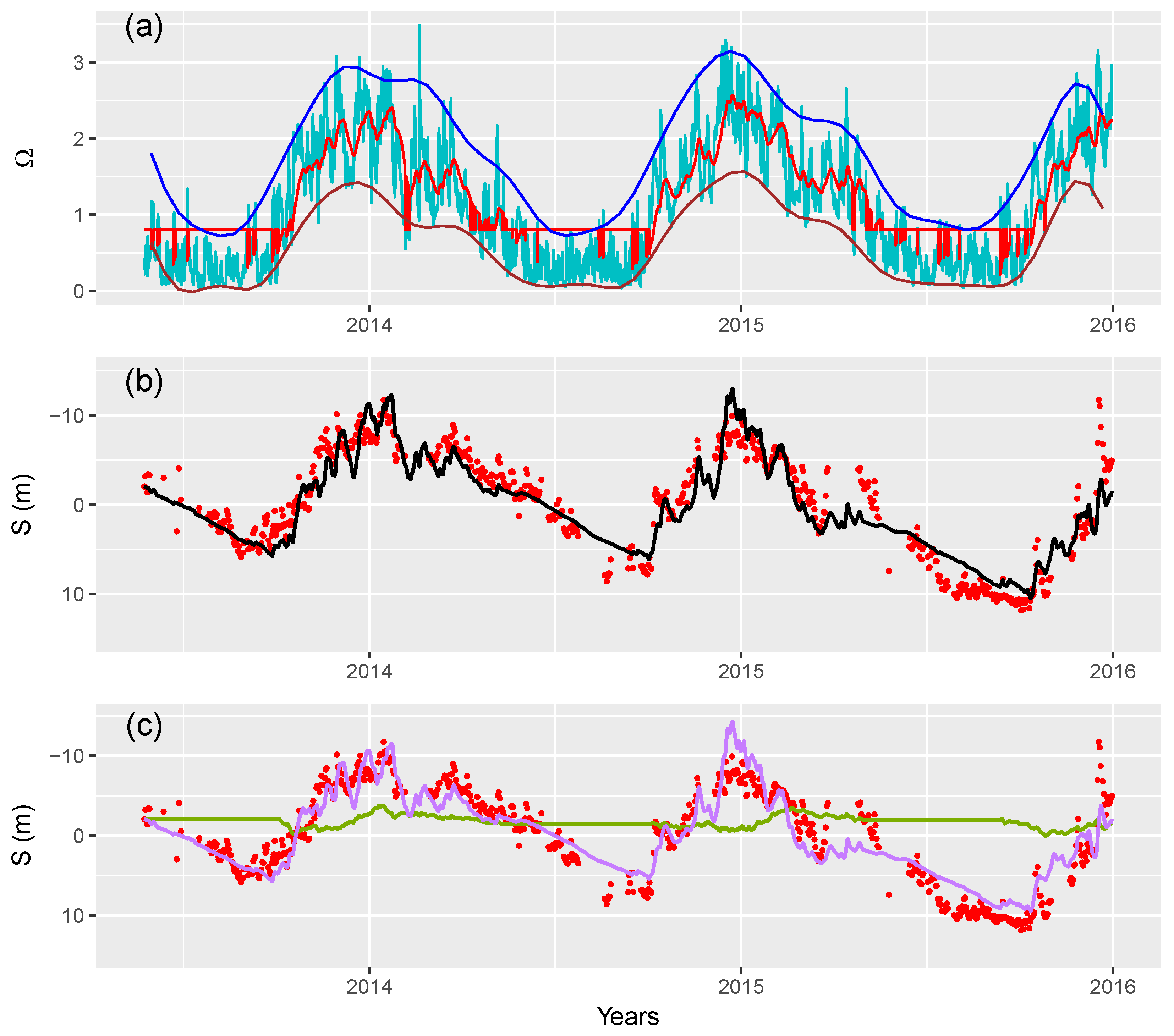
4. Application, Result and Discussion
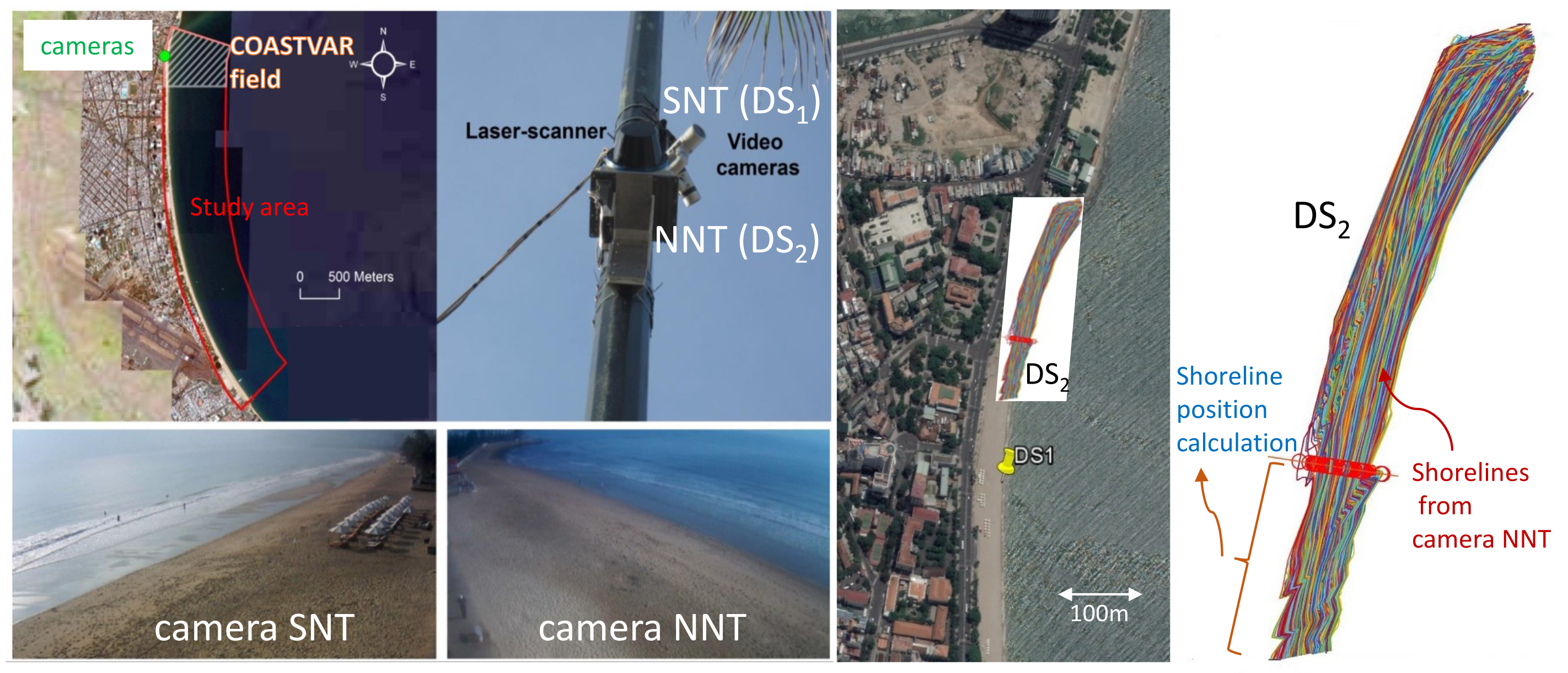
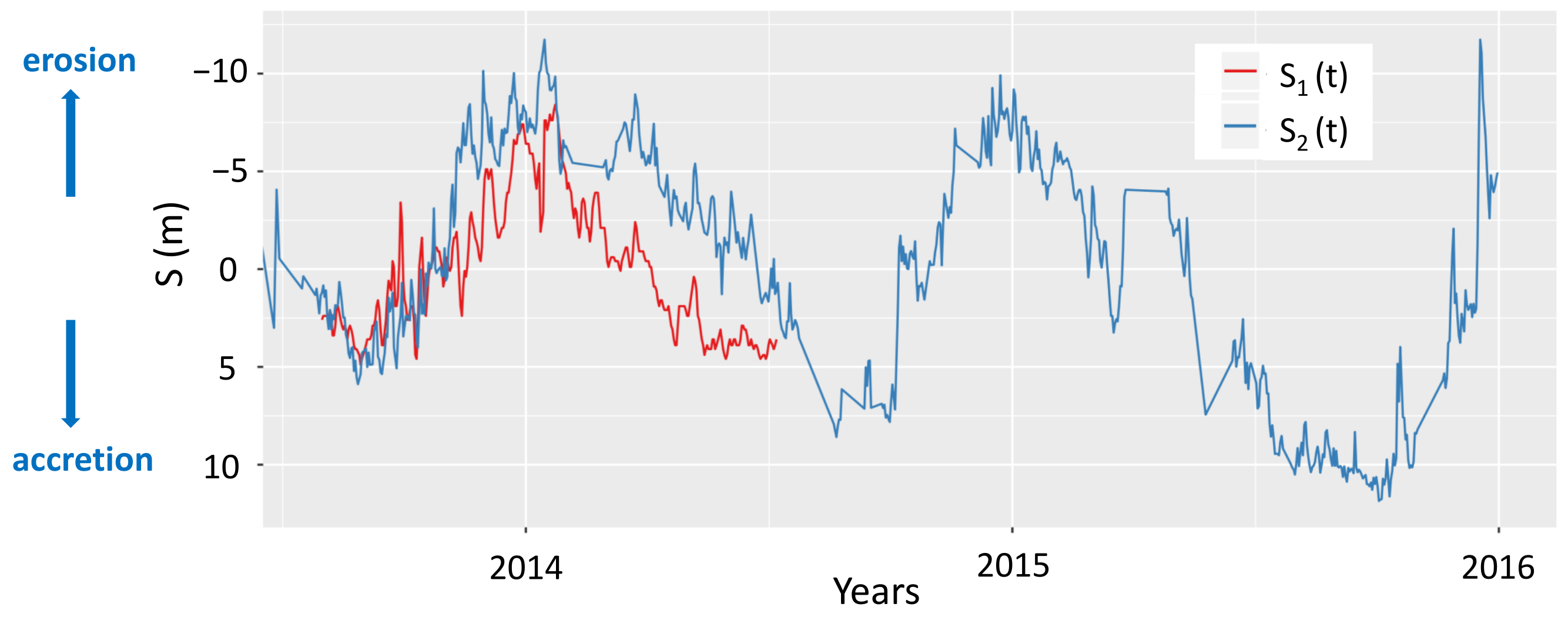
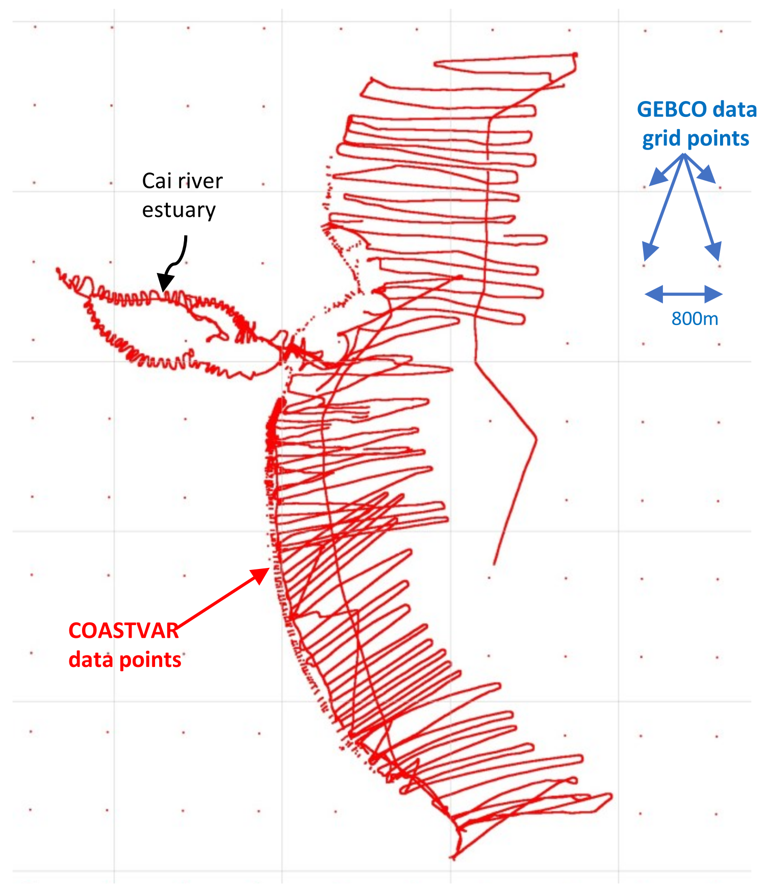
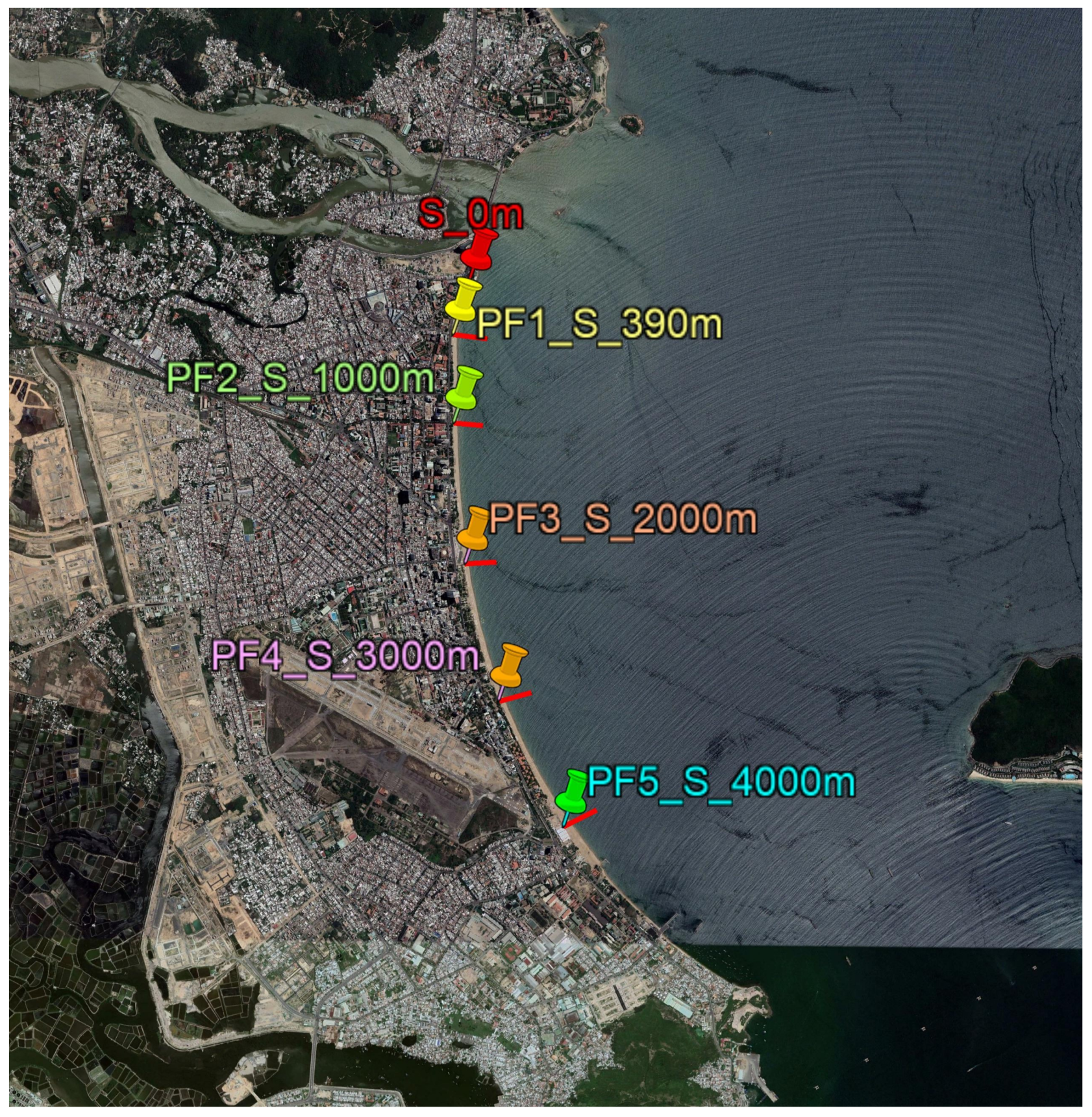
4.1. Shoreline Data
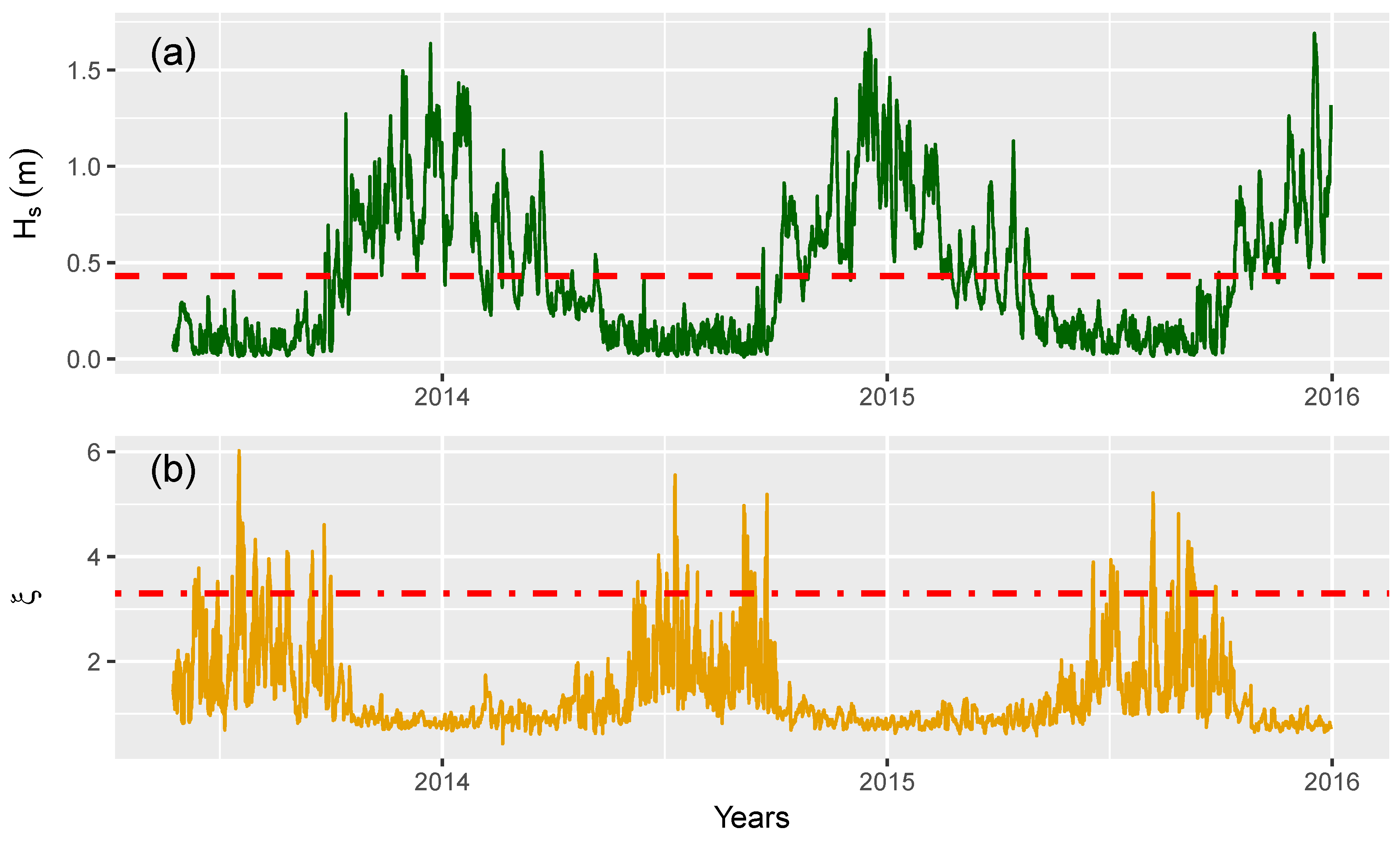
4.2. Wave Input Data
4.3. Result
4.4. Discussion
5. Conclusions
Author Contributions
Funding
Institutional Review Board Statement
Informed Consent Statement
Data Availability Statement
Acknowledgments
Conflicts of Interest
Abbreviations
| COASTVAR | Coastal Variability in West Africa and Vietnam |
| CosMos-COAST | Coastal One-line Assimilated Simulation Tool |
| ECMWF | European Center for Medium-Range Weather Forecasts |
| GEBCO | General Bathymetric Chart of the Oceans |
| RMSE | root mean square error |
| SWAN | Simulating WAves Nearshore model |
References
- Tran, Y.H.; Barthélemy, E. Combined longshore and cross-shore shoreline model for closed embayed beaches. Coast. Eng. 2020, 158, 103692. [Google Scholar] [CrossRef]
- Hanson, H.; Kraus, N.C. GENESIS: Generalized Model for Simulating Shoreline Change. Report 1. Technical Reference; Coastal Engineering Research Center: Vicksburg, MS, USA, 1989. [Google Scholar]
- Davidson, M.A.; Turner, I.L. A behavioral template beach profile model for predicting seasonal to interannual shoreline evolution. J. Geophys. Res. Earth Surf. 2009, 114. [Google Scholar] [CrossRef]
- Castelle, B.; Marieu, V.; Bujan, S.; Ferreira, S.; Parisot, J.; Capo, S.; Sénéchal, N.; Chouzenoux, T. Equilibrium shoreline modelling of a high-energy mesomacrotidal multiple-barred beach. Mar. Geol. 2014, 347, 85–94. [Google Scholar] [CrossRef]
- Splinter, K.D.; Turner, I.L.; Davidson, M.A.; Barnard, P.; Castelle, B.; Oltman-Shay, J. A generalized equilibrium model for predicting daily to interannual shoreline response. J. Geophys. Res. Earth Surf. 2014, 119, 1936–1958. [Google Scholar] [CrossRef] [Green Version]
- Vitousek, S.; Barnard, P.L.; Limber, P.; Erikson, L.; Cole, B. A model integrating longshore and cross-shore processes for predicting long-term shoreline response to climate change. J. Geophys. Res. Earth Surf. 2017, 122, 782–806. [Google Scholar] [CrossRef]
- Robinet, A.; Idier, D.; Castelle, B.; Marieu, V. On a reduced-complexity shoreline change model combining longshore and cross-shore processes: The LX-Shore model. Environ. Model. Softw. 2018, 109, 1–16. [Google Scholar] [CrossRef]
- Montaño, J.; Coco, G.; Antolínez, J.A.; Beuzen, T.; Bryan, K.R.; Cagigal, L.; Castelle, B.; Davidson, M.A.; Goldstein, E.B.; Vos, K.; et al. Blind testing of shoreline evolution models. Sci. Rep. 2020, 10, 2137. [Google Scholar] [CrossRef] [PubMed] [Green Version]
- Tomasicchio, G.R.; Francone, A.; Simmonds, D.J.; D’Alessandro, F.; Frega, F. Prediction of Shoreline Evolution. Reliability of a General Model for the Mixed Beach Case. J. Mar. Sci. Eng. 2020, 8, 361. [Google Scholar] [CrossRef]
- Roelvink, J.A.; Van Banning, G.K.F.M. Design and development of delft3d and application to coastal morphodynamics. Oceanogr. Lit. Rev. 1995, 11, 925. [Google Scholar]
- Roelvink, D.; Reniers, A.J.H.M.; Van Dongeren, A.; Van Thiel de Vries, J.; Lescinski, J.; McCall, R. Xbeach model description and manual. Unesco-Ihe Inst. Water Educ. Deltares Delft Univ. Technol. Rep. June 2010, 21, 2010. [Google Scholar]
- Warren, I.R.; Bach, H.K. Mike 21: A modelling system for estuaries, coastal waters and seas. Environ. Softw. 1992, 7, 229–240. [Google Scholar] [CrossRef]
- Yates, M.L.; Guza, R.T.; O’reilly, W.C. Equilibrium shoreline response: Observations and modeling. J. Geophys. Res. Ocean. 2009, 114. [Google Scholar] [CrossRef] [Green Version]
- Davidson, M.A.; Splinter, K.D.; Turner, I.L. A simple equilibrium model for predicting shoreline change. Coast. Eng. 2013, 73, 191–202. [Google Scholar] [CrossRef]
- Kriebel, D.L.; Dean, R.G. Convolution method for time-dependent beach-profile response. J. Waterw. Port Coast. Ocean. Eng. 1993, 119, 204–226. [Google Scholar] [CrossRef]
- Wright, L.D.; Short, A.D. Morphodynamic variability of surf zones and beaches: A synthesis. Mar. Geol. 1984, 56, 93–118. [Google Scholar] [CrossRef]
- Schepper, R.; Almar, R.; Bergsma, E.; de Vries, S.; Reniers, A.; Davidson, M.; Splinter, K. Modelling Cross-Shore Shoreline Change on Multiple Timescales and Their Interactions. J. Mar. Sci. Eng. 2021, 9, 582. [Google Scholar] [CrossRef]
- Pelnard-Considère, R. Theoretical Tests on the Shoreline Evolution of Sand and Gravel Beaches. In Proceedings of the 4èmes Journées de l’Hydraulique, Paris, France, 13–15 June 1956; pp. 289–298. [Google Scholar]
- Turki, I.; Medina, R.; Coco, G.; Gonzalez, M. An equilibrium model to predict shoreline rotation of pocket beaches. Mar. Geol. 2013, 346, 220–232. [Google Scholar] [CrossRef]
- Dronkers, J. Dynamics of Coastal Systems; World Scientific: Singapore, 2005; Volume 25. [Google Scholar]
- Coastal Engineering Research Center (US). Shore Protection Manual; Department of the Army, Waterways Experiment Station, Corps of Engineers, Coastal Engineering Research Center: Washington, DC, USA, 1984.
- Ashton, A.; Murray, A.B.; Arnoult, O. Formation of coastline features by large-scale instabilities induced by high-angle waves. Nature 2001, 414, 296–300. [Google Scholar] [CrossRef]
- Hurst, M.D.; Barkwith, A.; Ellis, M.A.; Thomas, C.W.; Murray, A.B. Exploring the sensitivities of crenulate bay shorelines to wave climates using a new vector-based one-line model. J. Geophys. Res. Earth Surf. 2015, 120, 2586–2608. [Google Scholar] [CrossRef] [Green Version]
- Roelvink, D.; Huisman, B.; Elghandour, A.; Ghonim, M.; Reyns, J. Efficient modelling of complex sandy coastal evolution at monthly to century time scales. Front. Mar. Sci. 2020, 7, 535. [Google Scholar] [CrossRef]
- Medellin, G.; Torres-Freyermuth, A.; Tomasicchio, G.R.; Francone, A.; Tereszkiewicz, P.A.; Lusito, L.; Palemon-Arcos, L.; Lopez, J. Field and Numerical Study of Resistance and Resilience on a Sea Breeze Dominated Beach in Yucatan (Mexico). Water 2018, 10, 1806. [Google Scholar] [CrossRef] [Green Version]
- Bruun, P. Sea-level rise as a cause of shore erosion. J. Waterw. Harb. Div. 1962, 88, 117–130. [Google Scholar] [CrossRef]
- Thuan, D.H.; Almar, R.; Marchesiello, P.; Viet, N.T. Video Sensing of Nearshore Bathymetry Evolution with Error Estimate. J. Mar. Sci. Eng. 2019, 7, 233. [Google Scholar] [CrossRef] [Green Version]
- Marchesiello, P.; Kestenare, E.; Almar, R.; Boucharel, J.; Nguyen, N.M. Longshore drift produced by climate-modulated monsoons and typhoons in the South China Sea. J. Mar. Syst. 2020, 211, 103399. [Google Scholar] [CrossRef]
- Almar, R.; Marchesiello, P.; Almeida, L.P.; Thuan, D.H.; Tanaka, H.; Viet, N.T. Shoreline response to a sequence of typhoon and monsoon events. Water 2017, 9, 364. [Google Scholar] [CrossRef] [Green Version]
- Bertsimas, D.; Tsitsiklis, J. Simulated annealing. Stat. Sci. 1993, 8, 10–15. [Google Scholar] [CrossRef]
- Thuan, D.H.; Binh, L.T.; Viet, N.T.; Hanh, D.K.; Almar, R.; Marchesiello, P. Typhoon impact and recovery from continuous video monitoring: A case study from Nha Trang Beach, Vietnam. J. Coast. Res. 2016, 75, 263–267. [Google Scholar] [CrossRef]
- Almeida, L.P.; Almar, R.; Blenkinsopp, C.; Senechal, N.; Bergsma, E.; Floc’h, F.; Caulet, C.; Biausque, M.; Marchesiello, P.; Grandjean, P.; et al. Lidar Observations of the Swash Zone of a Low-Tide Terraced Tropical Beach under Variable Wave Conditions: The Nha Trang (Vietnam) COASTVAR Experiment. J. Mar. Sci. Eng. 2020, 8, 302. [Google Scholar] [CrossRef]
- Andriolo, U.; Almeida, L.P.; Almar, R. Coupling terrestrial LiDAR and video imagery to perform 3D intertidal beach topography. Coast. Eng. 2018, 140, 232–239. [Google Scholar] [CrossRef]
- Tran, H.Y. Modeling Long Term Shoreline Evolution and Coastal Erosion. Ph.D. Thesis, Université Grenoble Alpes, Grenoble, France, 2018. [Google Scholar]
- Booij, N.R.R.C.; Ris, R.C.; Holthuijsen, L.H. A third-generation wave model for coastal regions: 1. Model description and validation. J. Geophys. Res. Ocean. 1999, 104, 7649–7666. [Google Scholar] [CrossRef] [Green Version]
- Bertin, X.; Castelle, B.; Chaumillon, E.; Butel, R.; Quique, R. Longshore transport estimation and inter-annual variability at a high-energy dissipative beach: St. Trojan beach, SW Oléron Island, France. Cont. Shelf Res. 2008, 28, 1316–1332. [Google Scholar] [CrossRef]
- Battjes, J.A. Surf similarity. In Proceedings of the 14th International Conference on Coastal Engineering, Copenhagen, Denmark, 24–28 June 1975; pp. 466–480. [Google Scholar]
- Galvin, C.J., Jr. Breaker type classification on three laboratory beaches. J. Geophys. Res. 1968, 73, 3651–3659. [Google Scholar] [CrossRef]
- Daly, C.; Floc’h, F.; Almeida, L.P.; Almar, R. Modelling accretion at Nha Trang Beach, Vietnam. Icoastal Dyn. 2017, 170, 1886–1896. [Google Scholar]
- Dalya, C.J.; Floc’h, F.; Almeida, L.P.; Almara, R.; Jaud, M. Morphodynamic modelling of beach cusp formation: The role of wave forcing and sediment composition. Geomorphology 2021, 389, 107798. [Google Scholar] [CrossRef]
- Davidson, M. Forecasting coastal evolution on time-scales of days to decades. Coast. Eng. 2021, 168, 103928. [Google Scholar] [CrossRef]
- Bird, E.C. Coastal Geomorphology: An Introduction; John Wiley & Sons: Hoboken, NJ, USA, 2011. [Google Scholar]
- Vos, K.; Harley, M.D.; Splinter, K.D.; Walker, A.; Turner, I.L. Beach Slopes from Satellite-Derived Shorelines. Geophys. Res. Lett. 2020, 47, e2020GL088365. [Google Scholar] [CrossRef]
- Bergsma, E.W.; Almar, R. Coastal coverage of ESA’Sentinel 2 mission. Adv. Space Res. 2020, 65, 2636–2644. [Google Scholar] [CrossRef]
- Taveneau, A.; Almar, R.; Bergsma, E.W.; Sy, B.A.; Ndour, A.; Sadio, M.; Garlan, T. Observing and Predicting Coastal Erosion at the Langue de Barbarie Sand Spit around Saint Louis (Senegal, West Africa) through Satellite-Derived Digital Elevation Model and Shoreline. Remote Sens. 2021, 13, 2454. [Google Scholar] [CrossRef]


| Transect | b | ||||||
|---|---|---|---|---|---|---|---|
| PF1 | |||||||
| PF2 | |||||||
| PF3 | |||||||
| PF4 | |||||||
| PF5 |
Publisher’s Note: MDPI stays neutral with regard to jurisdictional claims in published maps and institutional affiliations. |
© 2021 by the authors. Licensee MDPI, Basel, Switzerland. This article is an open access article distributed under the terms and conditions of the Creative Commons Attribution (CC BY) license (https://creativecommons.org/licenses/by/4.0/).
Share and Cite
Tran, Y.H.; Marchesiello, P.; Almar, R.; Ho, D.T.; Nguyen, T.; Thuan, D.H.; Barthélemy, E. Combined Longshore and Cross-Shore Modeling for Low-Energy Embayed Sandy Beaches. J. Mar. Sci. Eng. 2021, 9, 979. https://0-doi-org.brum.beds.ac.uk/10.3390/jmse9090979
Tran YH, Marchesiello P, Almar R, Ho DT, Nguyen T, Thuan DH, Barthélemy E. Combined Longshore and Cross-Shore Modeling for Low-Energy Embayed Sandy Beaches. Journal of Marine Science and Engineering. 2021; 9(9):979. https://0-doi-org.brum.beds.ac.uk/10.3390/jmse9090979
Chicago/Turabian StyleTran, Yen Hai, Patrick Marchesiello, Rafael Almar, Duc Tuan Ho, Thong Nguyen, Duong Hai Thuan, and Eric Barthélemy. 2021. "Combined Longshore and Cross-Shore Modeling for Low-Energy Embayed Sandy Beaches" Journal of Marine Science and Engineering 9, no. 9: 979. https://0-doi-org.brum.beds.ac.uk/10.3390/jmse9090979