Vehicle Routing Optimization of Instant Distribution Routing Based on Customer Satisfaction


1
School of Economics and Management, Beijing University of Posts and Telecommunications, Beijing 100876, China
2
School of Information Science and Technology, Zhejiang Sci-Tech University, Hangzhou 310018, China
*
Author to whom correspondence should be addressed.
Information 2020, 11(1), 36; https://0-doi-org.brum.beds.ac.uk/10.3390/info11010036
Submission received: 4 December 2019
/
Revised: 31 December 2019
/
Accepted: 6 January 2020
/
Published: 9 January 2020
Abstract
:Since the actual factors in the instant distribution service scenario are not considered enough in the existing distribution route optimization, a route optimization model of the instant distribution system based on customer time satisfaction is proposed. The actual factors in instant distribution, such as the soft time window, the pay-to-order mechanism, the time for the merchant to prepare goods before delivery, and the deliveryman’s order combining, were incorporated in the model. A multi-objective optimization framework based on the total cost function and time satisfaction of the customer was established. Dual-layer chromosome coding based on the deliveryman-to-node mapping and the access order was conducted, and the nondominated sorting genetic algorithm version II (NSGA-II) was used to solve the problem. According to the numerical results, when time satisfaction of the customer was considered in the instant distribution routing problem, the customer satisfaction increased effectively and the balance between customer satisfaction and delivery cost in the means of Pareto optimization were obtained, with a minor increase in the delivery cost, while the number of deliverymen slightly increased to meet the on-time delivery needs of customers.
1. Introduction
In the era of mobile internet, people can easily enjoy home delivery of commodities and services with the expansion of the scale of on-line shopping, which promotes the upgrading of the level of logistics and distribution services. As a newly emerged logistics distribution pattern under such circumstances, instant distribution has a most important feature which lies in its high requirement on timeliness. The delivery of goods is normally finished within 3 h, sometimes even within 30 min after the customer makes an order on the Internet. The prosperous development of instant distribution has also raised high demands on the logistics network. Therefore, optimization of logistics resources should be better deployed and optimized to make the delivery more efficient, the delivery cost lower, and the customers more satisfied.
Optimization of logistics distribution vehicle routing, also known as vehicle routing problems (VRPs), is a core optimization problem in the logistics network. It was first put forward by Dantzig and Ramser (1959), proposing a near optimal solution based on a linear programming formulation in the shortest routes [1]. The objective function [1,2] based on total mileage or total cost was widely used in the early stage, and then practical factors, such as vehicle capacity limitation [3], the multi-distribution center [4], the time window [5,6,7], costs of quality deterioration, and carbon emissions [8] were introduced. These factors made the objective conditions of vehicle routing optimization more closely combined with the actual problems.
In addition to these objective conditions, in recent years, more and more researchers have focused on introducing customer satisfaction factors into the distribution route optimization problem. Customer satisfaction refers to the matching degree between the user’s experience and the previous expectation in the process of using products and services. In instant distribution, consumers pay more attention to the service process time satisfaction of logistics distribution, that is, the impact of service time between customer order and delivery on customer satisfaction. Lan, et al. [9] distinguished order production, inventory-oriented production, mass customization production, and other evaluation criteria applicable to different customer satisfaction and used the fuzzy analytic hierarchy process (FAHP) to model customer satisfaction. Qianwen, et al. [10] proposed an improved fuzzy comprehensive evaluation method to measure customer satisfaction of takeaway distribution. Unlike most previous studies in literatures, Miranda, et al. [11] introduced a hard time window, random travel, and service time into the multi-objective vehicle routing problem, taking the minimum operating cost and maximizing the service level as optimization objectives. Daya, et al. [12] used the column generation heuristic algorithm to solve the vehicle routing problem. Miranda et al. [13] introduced a hard time window, random travel, and service time into the multi-objective vehicle routing problem and took the two conflicting objective functions of the minimum operating cost and maximum service level as optimization objectives.
The multi-objective vehicle routing problem (MOVRP) is an extension of VRPs. Time windows are introduced into VRPs in logistics distribution, resulting in a combinatorial optimization problem [14]. Different from single objective optimization, the optimal solution is a set of compromise solutions, namely the Pareto optimal solution set. The time window constraints may lead to total the distribution distance and number of service vehicles and may affect customer satisfaction [15]. Therefore, under the constraints of the time window, solving the problem of minimizing the distribution cost and maximizing customer satisfaction are usually two conflicting goals. When the minimizing of the routing cost and the maximizing of customer satisfaction are affected by the time window, customer satisfaction affected by too late arrival time and (possibly) too early arrival time has been modeled as a weighted combination of distribution cost and punishment of corresponding customer satisfaction in vehicle routing problem with time window (VRPTW) [16].
Researchers have proposed a series of multi-objective evolutionary algorithms (MOEAs) based on heuristic algorithms, such as the tabu search algorithm [14], genetic algorithm [17], simulated annealing algorithm [18], and ant colony algorithm [19], to solve the multi-objective vehicle routing problems. Deb [20] proposed the fast nondominated sorting genetic algorithm version II (NSGA-II) with elitist strategy based on the NSGA, and the algorithm has become a comparative mark for performance comparison of multi-objective optimization. It adopted the strategy of fast nondominated sorting and elite selection and selects the individuals with higher adaptability through crowding coefficient operators. Researchers proposed some improved versions based on the basic NSGA-II in Reference [20]. Tianyi, et al. [21] adopted the strategies of crossover, mutation, and elite reserve to design the hybrid NSGA-II to solve the problem of allocating vehicles with faster time and less cost.
Previous studies are mostly aimed at traditional logistics distribution networks. Meanwhile, the function of the service level assumes that distributors need to wait when they arrive at customer points in advance, which does not meet the requirements of soft time windows and extreme speed distribution in instant distribution scenarios. They usually directly aim at route optimization of instant distribution. There are few studies on this topic. However, the existing path optimization modeling methods have the following main drawbacks in the application of instant distribution systems.
Firstly, the above literature generally assumes that there are one or more fixed distribution centers. On the one hand, deliverymen usually live in relatively concentrated commercial centers, such as fixed distribution centers. On the other hand, there are some deliverymen scattered in various locations who can accept dispatch or snatch orders at any time. Therefore, it is necessary to consider the two situations of riding cohabitation and scattered riding, as well as the time when the deliveryman arrives at the merchant and the time when the merchant delivers the goods in the modeling.
Secondly, for the modeling of customer time satisfaction, symmetrical time windows are generally used in the existing literature, that is, the delivery time cannot be earlier than the earliest time expected by the user, nor later than the latest time expected by the user. Once the limit is exceeded, it is modeled as a penalty fee and added to the objective function. In instant distribution, users expect the sooner they arrive, the better. Therefore, the penalty cost of arriving too early does not accord with the reality of instant distribution.
Thirdly, considering that the cost of traditional logistics distribution often accounts for the main part of the distribution cost, the transportation cost is modeled as proportional to the distance traveled. But in instant distribution, logistics enterprises usually pay the freight by each order, which is called the pay-to-order mode. Within the typical urban service radius, the distance will not cause the difference of freight. This leads to the difference between the distribution mileage and the traditional distribution service, which is not reflected directly in the freight, but, due to the longer time for delivery, more transportation resources are occupied. In addition, the penalty cost beyond the expected time window of customers should also be considered.
Based on the particularity of the instant distribution scenario mentioned above, this paper establishes a comprehensive route optimization model of the instant distribution system, in view of the current situation that the existing research does not consider the particularity of the instant distribution scenario adequately. The impact of customer time satisfaction is considered in the proposed model. The innovation and contribution of this paper are mainly as follows:
- In view of the instant distribution service scenario, a route optimization model of the instant distribution system is proposed. In the model, the time when the deliveryman arrives at the merchant, the time needed for the delivery of the instant distribution merchant, and the upper limit of the deliveryman distribution are considered, which are in line with the actual situation of the instant distribution and are not included in previous research work.
- A customer time satisfaction function based on a one-sided soft time window is established as one of the objective functions. The total cost function of joint distribution is used to establish a multi-objective optimization model of instant distribution.
- In the total cost function, the distribution cost is calculated by the pay-to-order mode. The influence of mileage is reflected in the occupation of transportation resources, not directly converted into freight. The penalty function of time cost is designed based on the difference between the actual distribution time and the user’s expected latest delivery time.
The above model considers the particularity of instant distribution and adopts the above assumptions, which are more in line with the actual service scenario of instant distribution, which undoubtedly increases the credibility of the model and the applicability of the conclusions. After establishing the distribution routing optimization model of the instant distribution system, it is solved by the NSGA-II. In the design of the algorithm, a double-layer chromosome coding is established based on the mapping of deliverymen to nodes and the access order. The total cost and customer time satisfaction are jointly optimized in the sense of Pareto optimization. The results of the instant distribution route optimization model based on customer time satisfaction are compared and analyzed with those of the model without considering customer time satisfaction and only considering the total cost of distribution, and more conclusions are obtained. This research has important practical significance for optimizing resource allocation, reducing logistics costs, and improving logistics service levels and customer satisfaction of the instant distribution platform.
The rest of this paper is organized as follows. The problem of vehicle routing optimization is described according to the real instant distribution scenarios and the characteristics of instant distribution is analyzed in Section 2. In Section 3, we formulate a multi-objective optimization model for the instant distribution system based on the total cost function and time satisfaction of the customer and we take some actual factors of instant distribution into account. Dual-layer chromosome coding based on the deliveryman-to-node mapping and the access order was conducted, and the NSGA-II algorithm is used to solve the problem in Section 4. Numerical results are carried out in Section 5 to evaluate the performance. Finally, this paper concludes by identifying some potential researching points that can be carried out in future work.
2. Problem Description
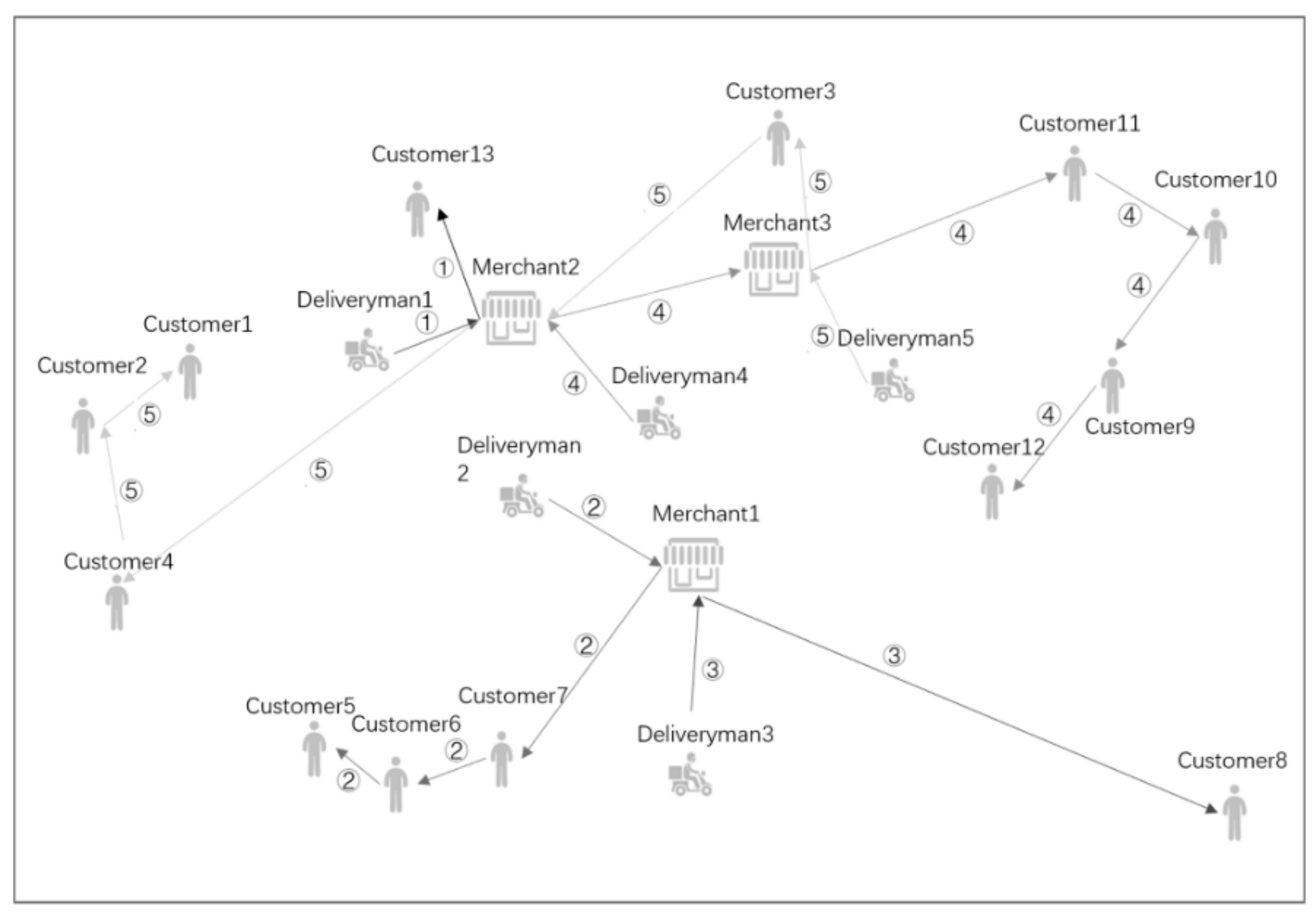
This research on the optimization of instant distribution routing is mainly about constructing the best distribution routes between multiple merchants and multiple customers under a time window for the process from the customer’s making an order and the merchant’s receiving the order to the handover of the goods to the customer. To facilitate the study, it is assumed that there are multiple deliverymen near each merchant, most of whom gathering in concentrated business centers, and many deliverymen distributing dispersedly in various locations to receive or scramble orders at any time. In addition, it should also be considered that deliverymen must travel some distance before they arrive at the merchants. After receiving a customer’s order, the deliveryman would travel to the merchant’s location to get the goods and then quickly start the delivery of the goods to the customer. If the number of customers and the number of merchants are fixed, and only one merchant’s goods are ordered in each order, and a customer may order goods from different merchants by making more than one order, then the logic diagram of the instant distribution system is shown in Figure 1.
As can be seen from the figure above, the distribution route optimization problem in instant distribution is the allocation problem of the multi-user problem in multi-distribution centers. There are multiple deliverymen who departure from each merchant, and each deliveryman can carry multiple orders at the same time, which is quite different from the traditional warehouse distribution scenario. The typical scenario of warehouse distribution is that after the vehicle delivers the goods from the distribution center to a user demand point, it returns to the distribution center and then carries on the next delivery, and each vehicle only allocates goods to one user. However, in instant distribution, such one-to-one distribution service is obviously not conducive to the cost reduction of logistics enterprises, because the users of instant distribution are mostly in densely populated cities and the demand is sudden and large. The situation that a merchant distributes multiple orders to multiple users at the same time is the most widespread scenario, so a reasonable merge of multiple orders is needed. Consequently, the transportation capacity is saved and the cost is reduced. However, compared with the single delivery mode, the merge mode will inevitably delay the delivery time. But the instant distribution users have strict requirements for the delivery time. For example, if the takeaway orders are not arrived for more than an hour after they are ordered, not only the demand for the customer’s meals will not be effectively met, but also the temperature of the dishes will greatly discount the customer’s experience after such a long time. Therefore, the customer’s requirement for the delivery time is strictly constrained. Once the customer’s satisfaction drops to the minimum level that can be tolerated, they are likely to give poor comments to the merchants. As a result, the reduction of the reputation of the merchants will bring adverse effects to the follow-up operation. In turn, the merchants’ accountability to the logistics enterprises will seriously affect the income of the logistics enterprises, and they may even transfer to other logistics service providers, so the market share of the logistics enterprises could be affected. Therefore, in the instant distribution service scenario, customer time satisfaction is very important, and its performance characteristics and impact degree are quite different from the conventional logistics distribution. Therefore, we should not only pay attention to the distribution cost, but also ensure the customer’s time satisfaction. The basic starting point of this paper is to establish the logistics distribution route optimization problem in the instant distribution scenario.
The following assumptions should be considered in instant distribution:
- The merchant needs some time to prepare the goods before delivery. If the deliveryman arrives too early, he has to wait at the store, which will waste the transportation capacity. Therefore, the delivery time of the merchant should be taken into account when dispatching the deliveryman.
- The merchant’s handling ability is limited, and the maximum ability is known. In the scenario of instant delivery, merchants will reject new orders when there is a lack of service resources, which is different from the scenario of warehouse distribution in which new orders are only a matter of delivery sooner or later and are rarely rejected.
- The number of merchants and customers and their geographical locations are known. Locations are denoted by longitude and latitude. Although user requirements are bursting in the real scenario, assuming a known number of users is a reasonable approximation to simplify the problem and will not affect the validity of the model.
- Geographical locations where deliverymen are gathering in are known, and deliverymen in each location are given their serial numbers. In the scenario of instant delivery service, deliverymen tend to gather in fixed places, such as near large shopping malls, so that they can deliver the goods as soon as receiving orders from the merchants in the shopping malls in which they settle.
- Geographical locations where deliverymen are dispersedly distributing are known, and each deliveryman has a corresponding serial number. In addition to the settlement point, there is also the situation that the deliverymen are scattered in different places in instant delivery, and the deliverymen can take orders for both the outward journey and the return journey. This is different from the conventional warehouse logistics distribution scenario, in which vehicles return and take another order. While for instant delivery, delivering in this way is obviously difficult to ensure timeliness and may waste transportation capacity.
- The maximum number of orders that each deliveryman can deliver goods for is known, and the number is the same for all deliverymen. There is an upper limit to the number of delivery orders for each deliveryman, which is a feature of instant delivery. For the sake of simplifying the analysis, we assume that the upper limit of the number of delivery orders for all deliverymen is equal, without loss of generality.
- All customers are covered by the distribution system, so there is no customer who cannot be delivered goods to. This is also the characteristics of instant delivery, that is, the distribution system serves as an intermediate link and orders cannot be rejected.
- The stock cost, handling loss, and other types of goods costs are not considered. In a typical warehouse logistics distribution scenario, inventory cost, and loading and unloading loss cannot to be ignored. While, in the instant distribution scenario, these factors are not important. The vehicles are usually light so that there are no loading and unloading losses, and the goods usually have good packaging so that there is no cargo damage. The impact of inventory is also small, because the delivery of the order is only a matter of time and will not be stored for a long time.
- The transportation expense during the delivery of goods is paid in a “pay-to-order” way and is constant. This is another feature of instant delivery and is also a typical difference between instant delivery and conventional logistics distribution. In conventional logistics distribution, the cost of distribution is directly determined by distribution range, while in instant distribution, merchants tend to sign long-term cooperation contracts with logistics enterprises. The logistics enterprises are likely to pay a fixed freight to the logistics enterprises for each order. Therefore, the instant delivery system is more sensitive to delivery time than to actual mileage. Accordingly, we introduce the customer time satisfaction to the optimization model, which is more in line with the characteristics of instant delivery.
- All deliverymen are in a constant speed during the delivery, without consideration of changes of road conditions or influence of the weather. It is assumed that equal distribution speed of deliverymen is a reasonable approximation to the problem modeling. Although the weather and road conditions may impact the timeliness of instant delivery, they are not included in this work for simplicity.
3. Mathematical Model
Orders in an instant distribution system involve many unforeseen circumstances. There are normally a great amount of orders to be dealt within certain periods of time. Additionally, there are high requirements on timeliness for these orders. In addition, customer comments have a great influence. Therefore, customer satisfaction becomes a priority. Therefore, a multi-objective optimization model is established based on the consideration of customer satisfaction and total delivery cost.
It is assumed that the total number of merchants in the distribution system is , the total number of customers is , the total number of deliverymen is , the set of merchants is , the set of customers is , the set of deliverymen is , the average driving speed of deliverymen is , the maximum number of orders for deliverymen is , the -th merchant’s distribution demand quantity is , the maximum number of orders that the -th merchant can handle is , the number of orders demanded by the -th customer is , whether Deliveryman delivers goods from Merchant to Customer is (= 1 if yes, = 0 if no), whether Deliveryman passes Merchant is (= 1 if yes, = 0 if no), the distance between the -th deliveryman and the -th merchant is , the distance between the -th merchant and the -th customer is , the number of orders delivered from the -th merchant to the -th customer is , and the delivery cost of each order is yuan/order.
The instant distribution system is highly sensitive to time, so the time taken in the delivery process is included in the total cost. The time cost includes the time cost for the delivery process and the time cost for the deliveryman to reach the merchant and wait before the start of the delivery. The delivery time cost is the time for the deliveryman to arrive at the destination multiplied by the time cost coefficient. The waiting time cost is the time cost produced from the fact that the merchant does not finish the preparation of goods when the deliveryman arrives at the merchant’s location. In addition, when a customer makes an order, the latest goods handover time will be specified in the order, once the total delivery time exceeds the specified latest handover time, and some time penalty cost will be incurred. The excessive time window cost is the penalty fee incurred from the deliveryman’s failing to deliver the goods to the customer within the specified time. It is assumed that the time between Customer ’s making an order from Merchant and the start of the delivery of the goods is ; the time the deliveryman spends to arrive at Customer ’s place after he receives the order and starts from his place is ; the unit time cost coefficient is ; the latest time for the goods to be handed to Customer after he makes an order in Merchant is ; the penalty coefficient in case the deliveryman arrives at the customer’s place in a time exceeding the time window is .
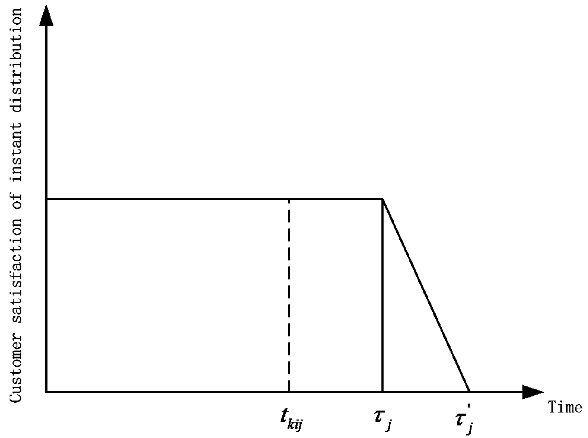
This paper focuses on the distribution of goods, so the influence of the quality of goods before their delivery starts is not considered. Meanwhile, modeling for customer satisfaction only has one judgement dimension, which is the delivery time. It is assumed that the time window for Customer ’ s receiving service from the i-th Merchant is . If deliveryman k arrives at the customer’s place later than the latest service ending time that the customer can accept, which is , the customer will be unsatisfied, leading to a reduction of customer satisfaction. It is noted that this customer satisfaction modeling method is different from the commonly used bilateral time window function. The bilateral time window function considers that customer expectation of distribution time has an expected range. Advance and lag will reduce satisfaction. It is suitable for routine logistics distribution scenarios, such as warehouse distribution, but not for instant distribution. However, in most cases, customers have some tolerance for the delay of goods handovers, but if the goods arrive before their expectation, customers usually do not care. It is assumed that the latest service time that a customer can tolerate is . Customer satisfaction is inversely proportional to the delayed service time, as shown in Figure 2.
Under the condition that the total delivery cost and customer satisfaction are considered comprehensively, the following multi-objective optimization model is established. The model includes two objective functions, namely, minimum total cost (minC) and maximum customer satisfaction (maxS):
Constraint conditions:
In this model, Objective (1) is the objective function of the total delivery cost. Item 1 on the right side of the equation is the total cost of the deliveryman from the merchant to the customer. Since it is paid on an order, this item has nothing to do with the distance. Item 2 is the total delivery time cost of the deliveryman from the merchant to the customer. The delivery time is calculated by dividing the distance from the merchant to the customer by the vehicle driving speed and then multiplying by the occupancy cost coefficient per unit time. Item 3 is the time cost of the deliveryman waiting at the merchant. If the delivery time of the merchant is less than or equal to the time of the deliveryman arriving at the merchant, there is no need to wait. The result of this item is 0. Otherwise, the time cost of this part is obtained by multiplying the difference between the delivery time of the merchant and the arrival time of the deliveryman by the occupancy cost coefficient per unit time. Item 4 is the penalty cost incurred when the total delivery time exceeds the latest handover time. Objective (2) is the objective function of customer time satisfaction, and the definition of time satisfaction is shown in Constraints (3) and (4), which is reflected as a kind of soft time window constraint. When the total delivery time is later than the end time of the service accepted by the customer, but not more than the service time tolerated by the customer, the customer time satisfaction is directly proportional to the difference between the service time tolerated by the customer minus the actual delivery time. When the delivery time exceeds the service time that the customer can tolerate, the customer time satisfaction drops to 0. Constraint (5) defines as a variable of 0–1, indicating whether there is a distribution relationship between Deliveryman distribution from Merchant to Customer . If there is a distribution relationship, take 1, otherwise, take 0. Constraint (6) restricts the number of orders delivered by each deliveryman to an upper limit of . Constraint (7) restricts the distribution of Deliveryman from Merchant to Customer . If there is a distribution relationship, it must simultaneously satisfy the requirement of passing through Merchant . Constraint (8) indicates that the total delivery time is equal to the sum of the time from the current position of the deliveryman to the merchant, the time for the deliveryman to wait at the merchant, and the time from the merchant to the customer. Constraint (9) restricts the order quantity of each merchant’s customers to be non-negative. Constraint (10) defines and as 0–1 variables. Constraint (11) indicates that the order quantity of each customer is equal to the sum of the orders placed by each merchant. Constraint (12) constrains the order quantity placed by the customer at the merchant not to exceed the upper limit of the total order quantity of the merchant.
4. Solution Methodology
4.1. NSGA-II
A genetic algorithm (GA) was adopted to solve the problem based on the single-objective programming model. The NSGA-II, which uses nondominated sorting, a crowding distance operator, and an elitist strategy, has many advantages, including maintaining population diversity, avoiding the loss of parent excellent individuals, and so on. It can constantly optimize the optimal solution set and is suitable for solving logistics distribution problems with the multi-objective optimization model [20].
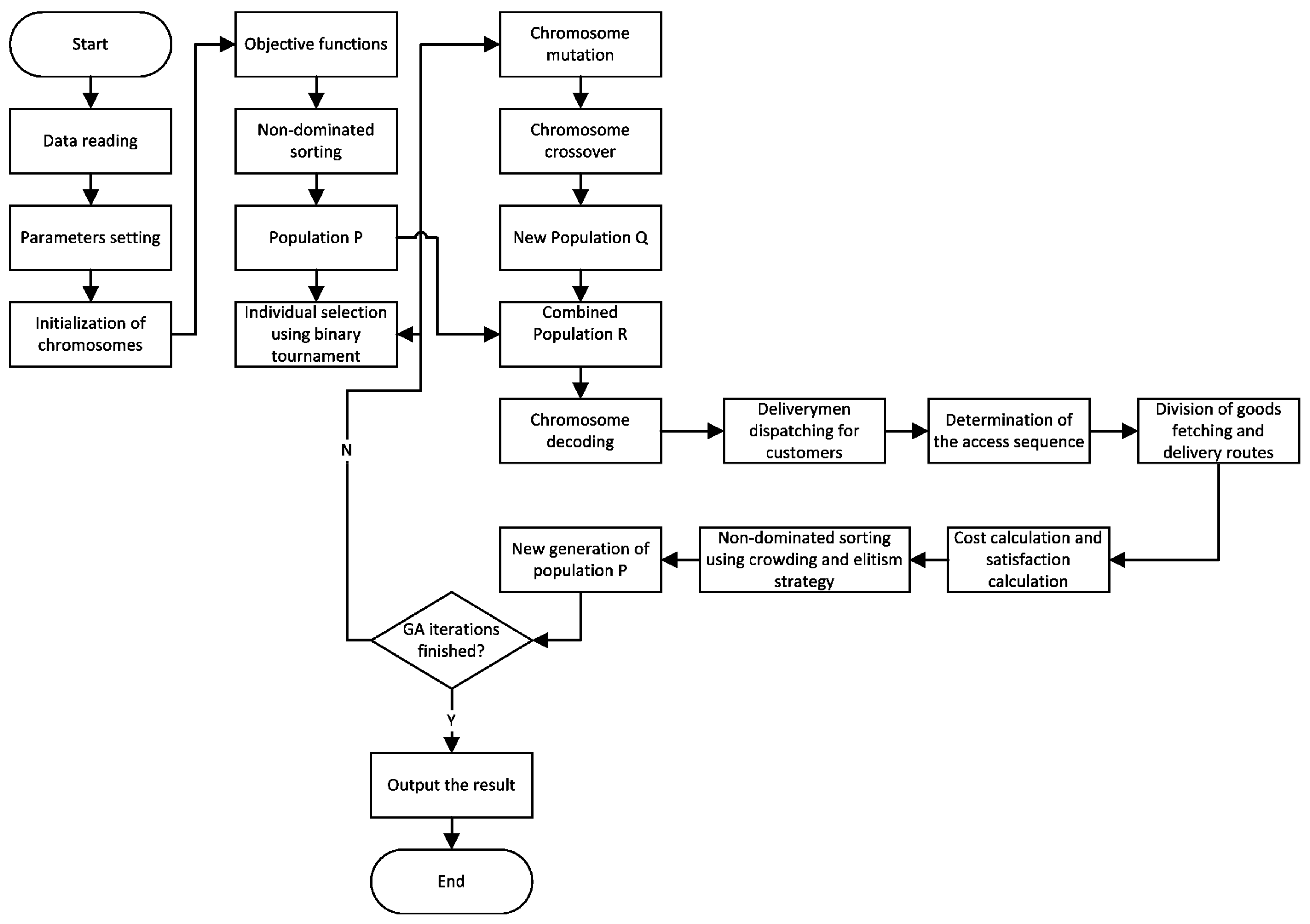
The solving procedures are as follows, as shown in Figure 3:
Step 1: The population algebra is set as . The population starts with random initialization. Nondominated sorting of is performed to initialize the rank value of each individual.
Step 2: The population algebra is set as .
Step 3: Individuals are selected from using binary tournament selection. Crossovers and variations are performed to generate the new generation of population .
Step 4: and are combined to generate the combination population .
Step 5: Nondominated sorting of is performed, with crowding and the elitism strategy used to select N individuals which form the new generation of population .
Step 6: Skip to Step 3 and a loop operation is performed until the end condition is met.
In Step 1 and Step 5 of the algorithm, a nondominated sort was used. Fast nondominated sorting was adopted to stratify the population according to the level of non-inferior solutions of individuals to make the solution close to the Pareto optimal solution. This was a process of adaptive value grading, circularly. First, the dominant groups in the solution set were constructed, denoted by . Then, the i-th individual was given a nondominated rank, denoted by the , which was set to 1 and removed from the group. We continued to get the nondominated solution set in the rest of the group, denoted by , and the individuals in were given = 2, so we continued until the entire population was layered.
The selection strategy in Step 3 adopts the binary championship method. A certain number of individuals were taken out of the population at a time for sampling back, and then the individual with the best crowding metric was selected to enter the offspring population. The process was repeated until the new population size reached the original population size.
The mutation operation in Step 3 was implemented by a 2-interchange mutation operator. Firstly, two random natural numbers and were generated, and then the and genes were exchanged to realize the mutation process. The crossover operation adopted a two-point crossover. Firstly, two chromosomes were randomly selected as the male parent to produce two random natural numbers and . Then, the gene fragments between the two male chromosomes and were exchanged to obtain two progeny chromosomes.
Compared with the basic NSGA, the improvements of NSGA-II mainly lie in three aspects: Firstly, adopting the fast nondominated sorting algorithm, which greatly reduces the complexity of the algorithm; secondly, putting forward the crowding strategy, which uses the crowding degree and crowding degree comparison operator, instead of the fitness sharing strategy in the NSGA algorithm; thirdly, adopting the elite retention strategy, which can retain the superiority of the parent as much as possible and avoid losing the best individuals.
4.2. Detailed Design
Detailed design of using the NSGA-II to solve instant distribution routing problems was performed. The design is mainly for designing chromosome coding and decoding processes.
The chromosome coding process was completed during population initialization. The coding method is as follows:
Double layer coding is performed for demand points, deliverymen, and merchants. The first layer coding is to specify the deliverymen belonging to corresponding nodes. It shows which deliveryman should serve which node, using integer coding with a length of . The genetic locus is an integer [1,], denoting which deliveryman serves a specific node. The second layer coding is to specify the node access sequence. The coding length is ,which is a non-repetitive sorting of integers 1~, where represents the total number of orders. For example, if = 4 = 3, a legal chromosome can be represented as [1,3,3,2,5,4,2,1,3,6]. The first layer coding of deliverymen belonging to various nodes is represented as 1,3,3,2, meaning that node 1 is served by deliveryman 1, node 2 is served by deliveryman 3, node 3 is served by deliveryman 3, node 4 is served by deliveryman 2, and so on. The second layer coding for the node access sequence is represented as 5,4,2,1,3,6, meaning that node 5 is the first to be accessed, followed by node 4, node 2, and so on. The division of subpaths is also in such an order, according to the deliveryman’s loading limitation and time window.
The chromosome decoding process is as follows:
- All serial numbers of nodes served by deliveryman 1 are fetched according to their sequence in chromosome to get the serial numbers of nodes served by each deliveryman ();Division of routes for is performed;
- The division starts from the first node in ;
- When a node is arrived at, it is judged if the deliveryman can load all the goods in the node. If so, the goods will be loaded and the distribution quantity of the demand point will be emptied, and then skip to (d). If not, skip to (c);
- Partially delivered goods in the demand point are loaded, until the vehicle is full, and then the distribution quantity of the demand point will be updated. The deliveryman then travels to the location of customer and then returns to the node. When the process is finished, skip to (b);
- It is judged if all the nodes have been accessed. If not, the deliveryman will go to the next node, and then skip to (b). If so, skip to (e);
- The access path and the deliveryman’s loading situation are the output.
- Path calculation is performed according to the access path and the deliveryman’s loading situation obtained in A.
In addition, at the stage of chromosome variation, different variation methods were adopted for the first layer coding and second layer coding. Single variation was adopted for the first layer coding. A random natural number was generated. The number denoted that the gene in the position was mutated. Random variation was used to make the gene in the position mutated. Double-point reciprocity was adopted for the mutation in the second layer coding. Two random natural numbers were generated. The genes in the and positions were exchanged. At the stage of chromosome selection, the selection was performed through roulette selection.
In the above algorithm, the distribution path was represented by chromosome coding, which included two segments from the location of the deliveryman (including the two types of location of the deliveryman settlement and the deliveryman scattering point) to the merchant and from the merchant to the user. This was the characteristic of the instant distribution system, which was different from the traditional logistics distribution service. In a typical warehouse distribution scenario, the distribution path incorporates only the distance from the distribution center to the user demand point. There are two segments in the coding process of instant delivery, which introduces more complexity. In addition, in the decoding process, it also reflects the important feature that there is a ceiling on the number of delivery orders per deliveryman in instant distribution.
5. Numerical Results and Discussions
5.1. Parameter Setting
The dataset in this study comes from the real distribution network of a Chinese takeout delivery company. The data was collected during the lunch period in the downtown area of the city. The application scenario of this example was a high-frequency scenario instant delivery, so the research based on this example has strong representativeness for instant delivery. In the dataset, there were 31 customers, five merchants, three gathering points of deliverymen, four disperse distribution points of deliverymen, and 28 deliverymen, and the deliverymen gathering points, 1,2,3, corresponded to deliveryman numbers 1–8, 9–16, and 17–24, respectively, and the four disperse distribution points of deliverymen corresponded to deliverymen 25–28. Locations of merchants, customers, and deliverymen were all provided in longitude and latitude. Each customer made orders from different merchants, and the same customer could make orders from different merchants separately. The total number of orders of customers was 49. The time for the goods to be delivered for different customers varied between 2 and 10 min. Customers expected the latest goods handover time to vary between 30 and 60 min. To save space in this paper, only some orders of merchant 1 are listed in Table 1.
In the example, the average driving speed of deliverymen was set as 20 km/h; the order’s unit delivery cost was set as 6 yuan/deal; the unit time cost coefficient was set as 18 yuan/h; the penalty coefficient for the deliveryman’s arrival time exceeding the time widow was set as 3; the longest goods handover time that demand point could tolerate was set as , of which was the expected longest handover time of point .
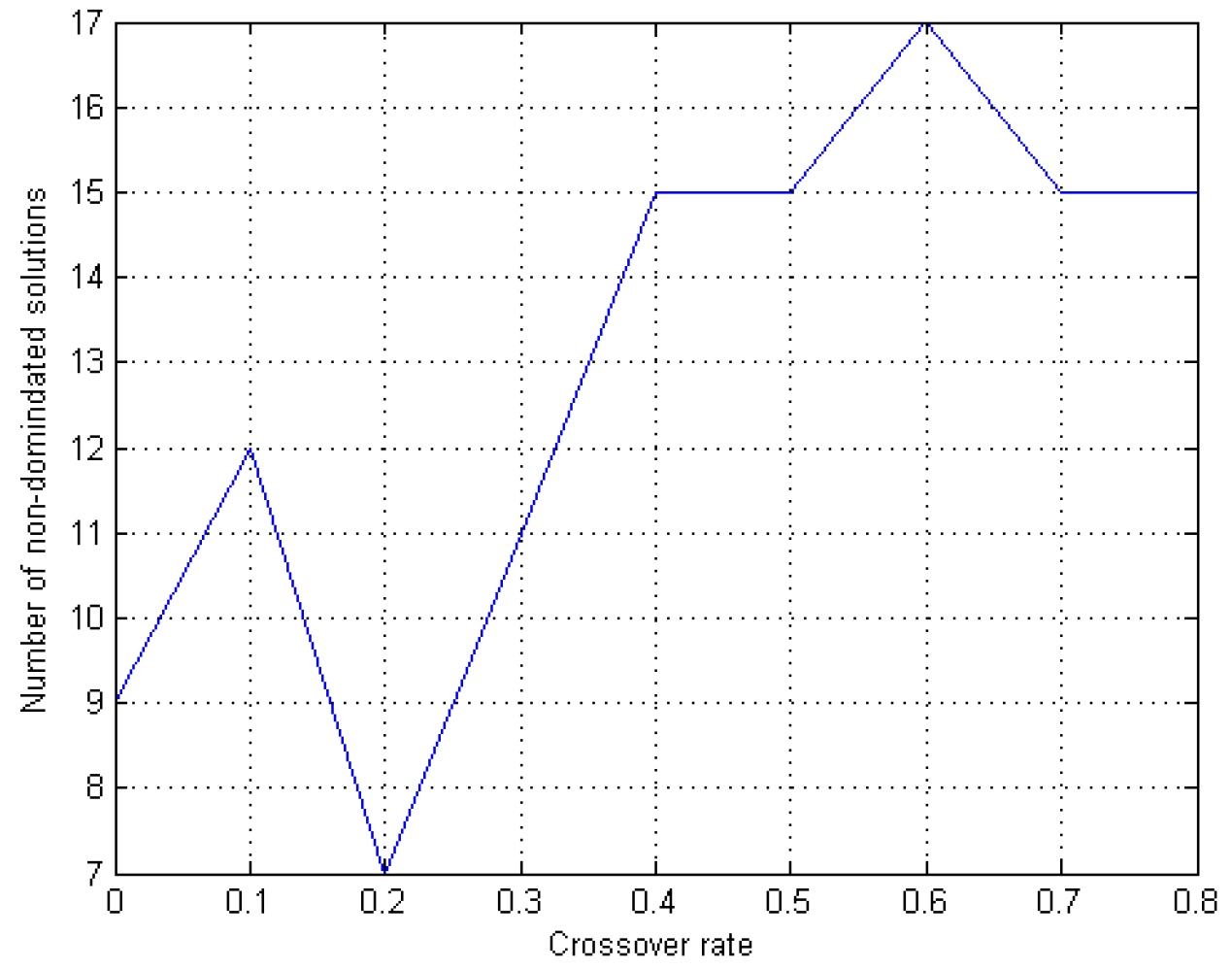
Since the parameters of the NSGA-II had a significant impact on the performance, we made some simulations to obtain the appropriate parameters. Firstly, the impact of mutation rate and crossover rate were studied through simulation, and the performance was evaluated by the number of nondominated solutions, i.e., more nondominated solutions meant better performance. The number of nondominated solutions obtained by the NSGA-II under different mutation rates and different crossover rates are shown in Figure 4 and Figure 5, respectively.
As can be seen from Figure 4, when the mutation rate was 0.2 and 0.4, the largest number of nondominated solutions could be obtained, which was 17. Therefore, the mutation rate set to 0.2 may be appropriate. As can be seen from Figure 5, when crossover rate was 0.6, the largest number of nondominated solutions could be obtained, which was 19. Therefore, the crossover rate should be set as 0.6.
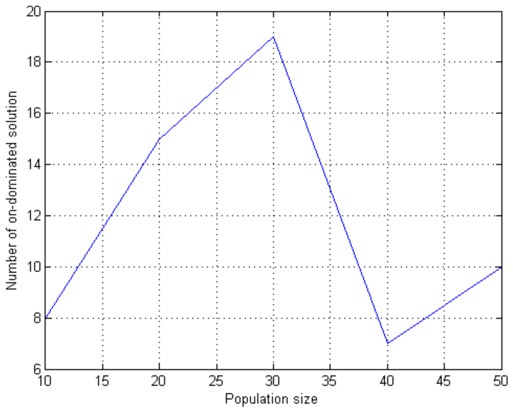
The impact of different population sizes on the performance was also simulated. Figure 6 shows the number of nondominated solutions obtained under different population sizes.
As can be seen from Figure 6, when the population size was 30, the maximum number of nondominated solutions could be obtained, which was 19. Therefore, in the subsequent simulations, the population size was set to 30.
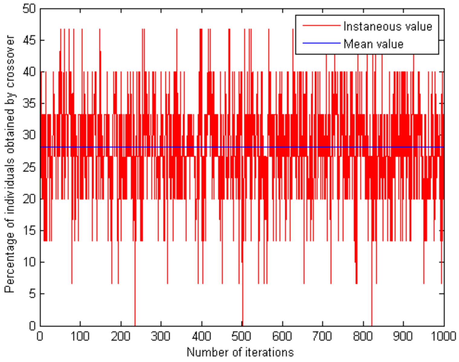
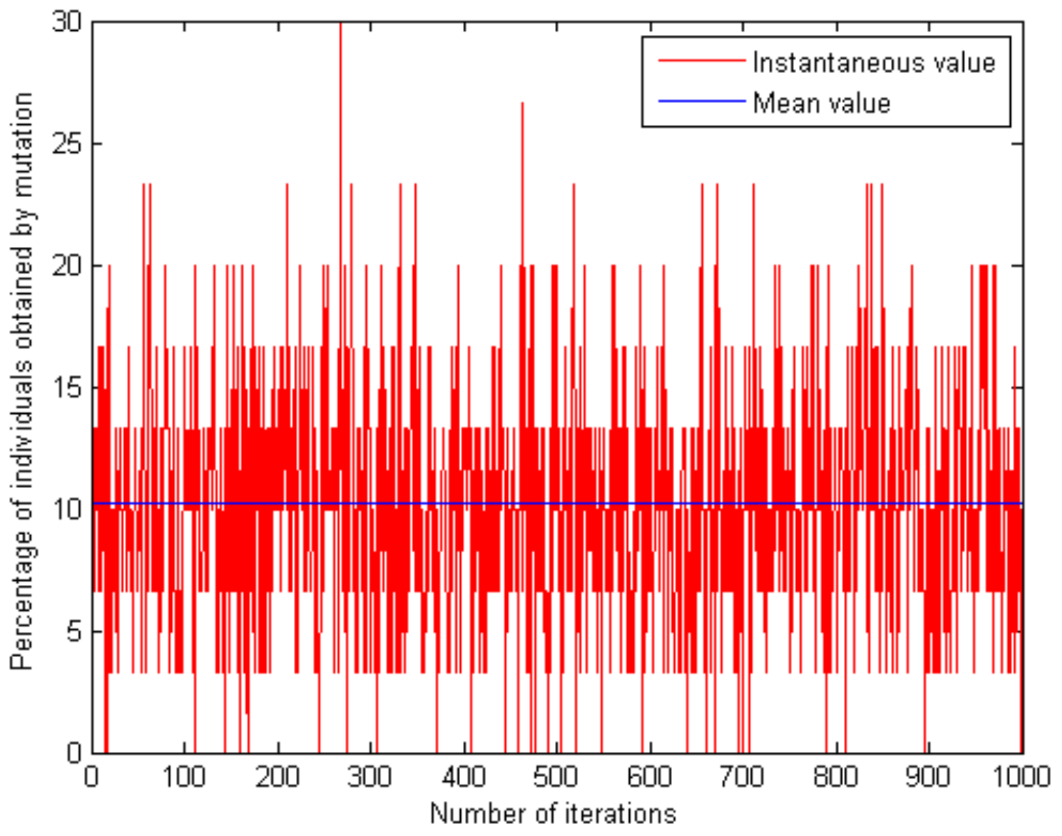
We also made some observations on details of the mutation and crossover process, as shown in Figure 7 and Figure 8, in which the red curves indicate the instantaneous values and the blue curves indicate the mean values.
As can be seen from the results in Figure 7 and Figure 8, the individual percentage of descendants obtained in the process of mutation was about 10% and the average percentage of descendants obtained in the process of crossover was about 28%, which were in a reasonable range.
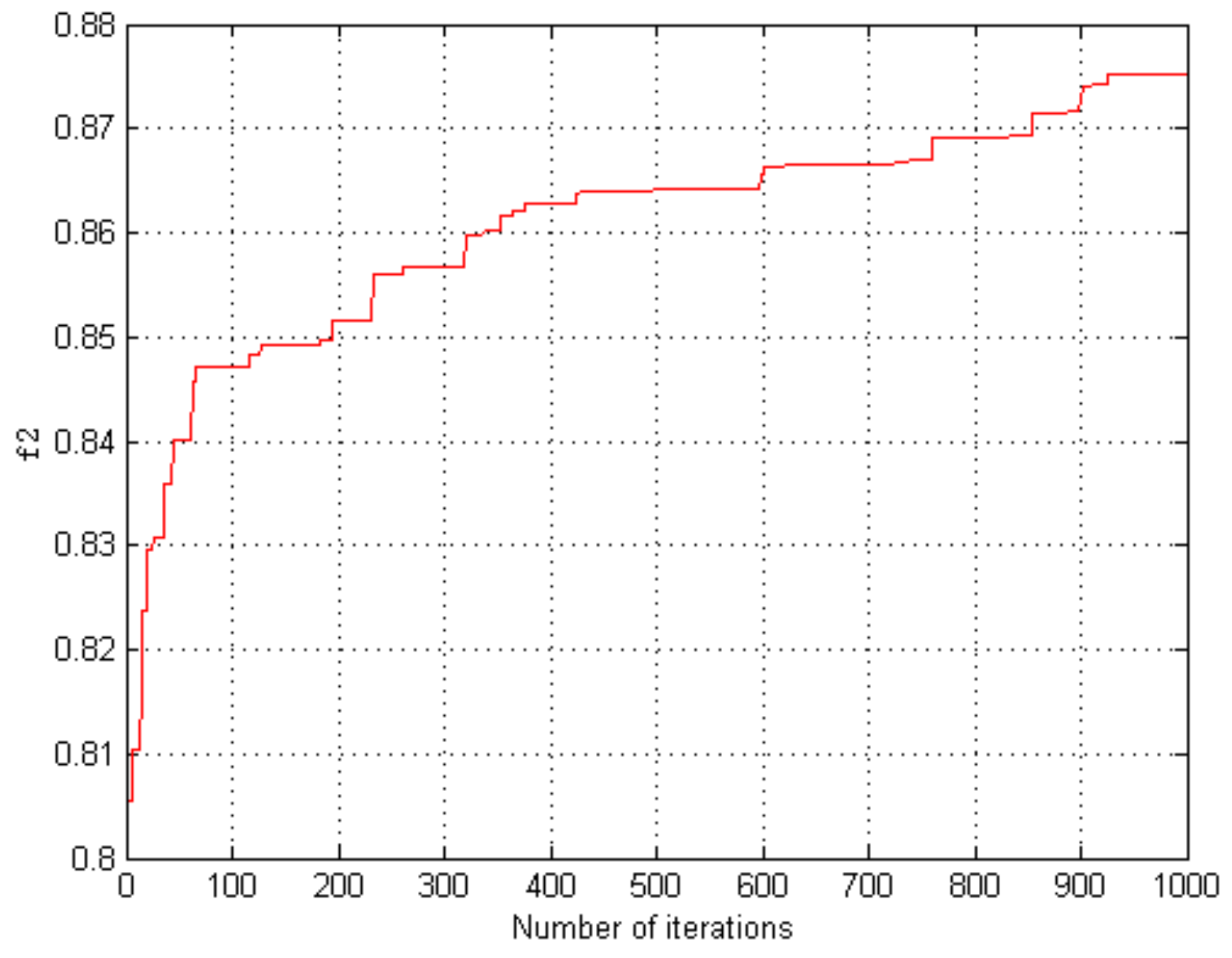
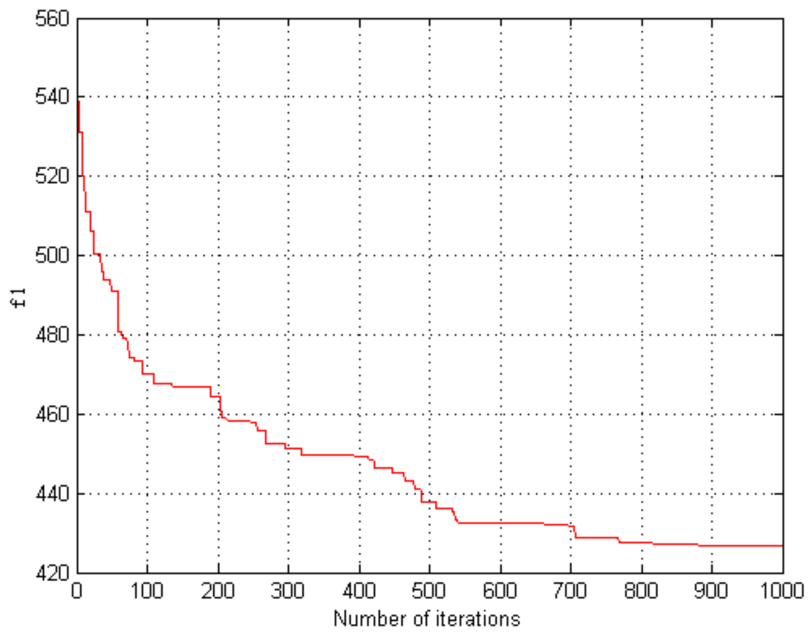
Finally, the influence of iteration times on performance was studied, as shown in Figure 9 and Figure 10, which are the convergence curves of the two objective functions of the NSGA-II.
It can be seen from the curves of Figure 9 and Figure 10 that the two objective functions had good convergence effects after 600 iterations, and 1000 was a proper value for both objective functions.
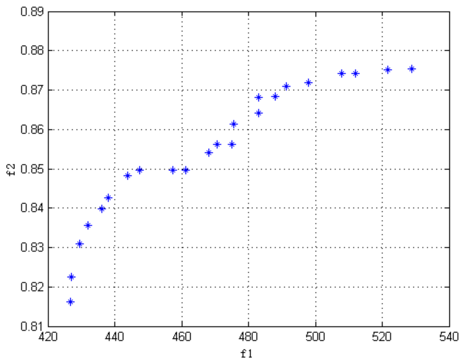
The Pareto front solution set for using the NSGA-II to optimize the objective functions of both the total cost and customer satisfaction is shown in Figure 11.
As can be seen from Figure 11, the parameters used in the algorithm had good optimal solution search ability.
Based on the simulations above, the parameters of the NSGA-II used in the following simulations are listed in Table 2.
5.2. Simulation Results
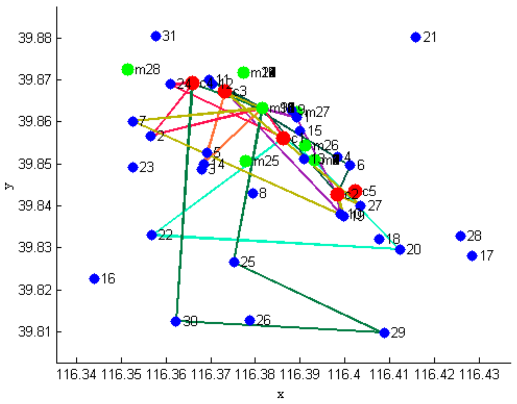
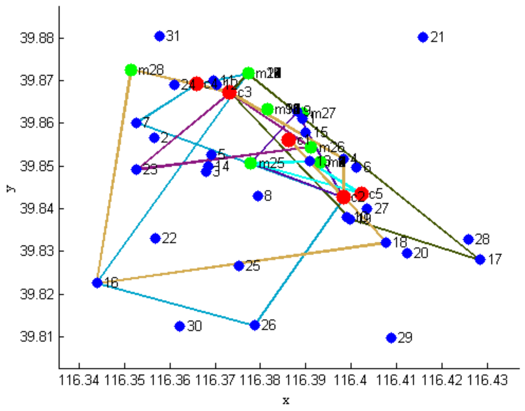
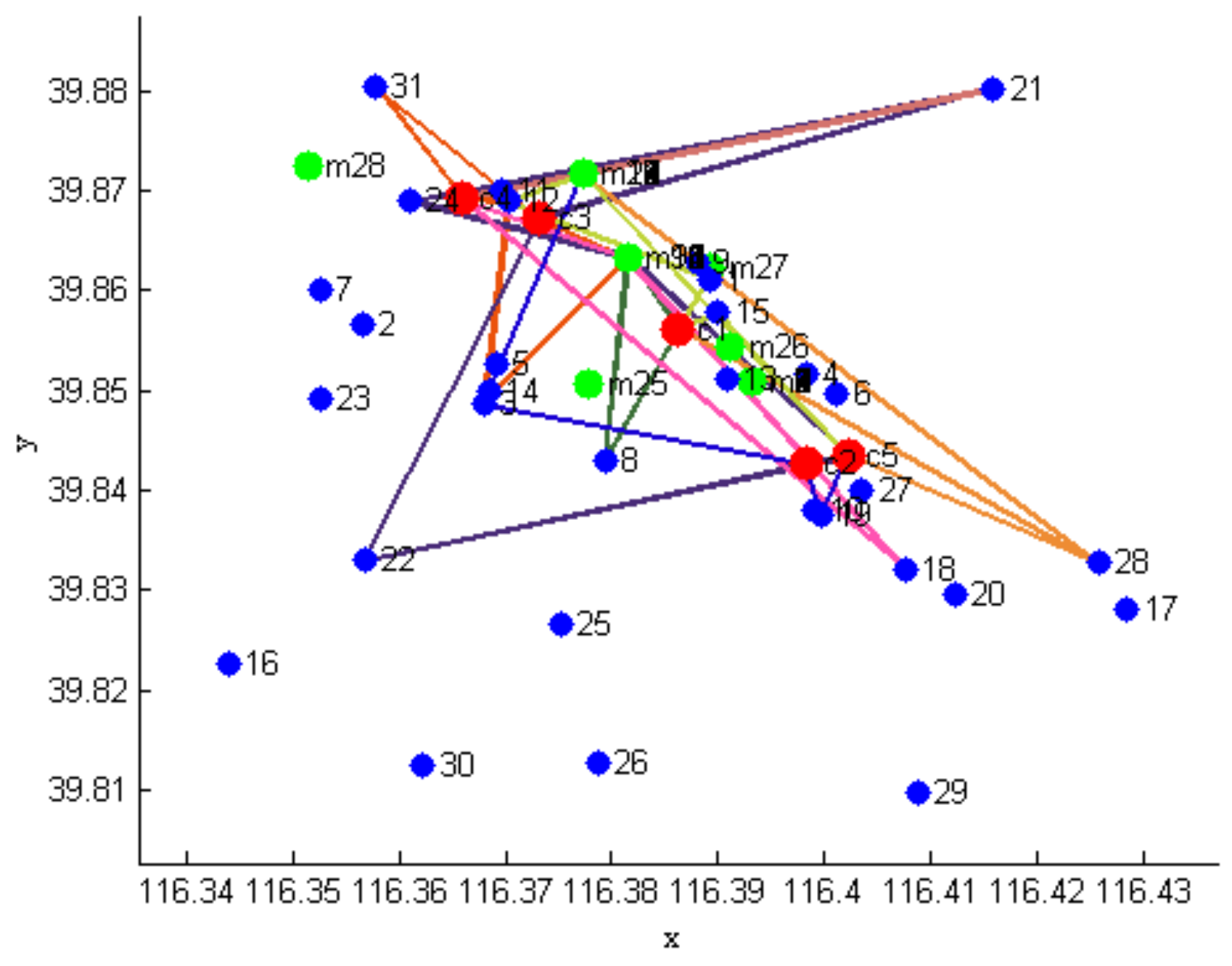
Distribution routes obtained using the NSGA-II are shown in Figure 12, Figure 13, Figure 14 and Figure 15. In each figure, the distribution routes of seven deliverymen are provided. Figure 12 gives the routes of deliverymen 1–7, and Figure 13 gives the routes of deliverymen 8–14, and so on.
In Figure 12, Figure 13, Figure 14 and Figure 15, the red markers represent the locations of deliverymen, the green points represent the locations of merchants, and the blue markers represent the locations of customers.
Furthermore, the distribution route results of the deliverymen are shown in Table 3, from which we can obtain more details, including order combination, as well as whether the deliveryman departed from a merchant and returned to the same merchant to continue the distribution of the next order, etc.
From the computational results of this example, it can be shown that the phenomenon of order combination exists widely. For most cases, the deliveryman took five orders mostly. There were also cases where a deliveryman continued to go to the same merchant’s for delivery of new orders after finishing the delivery of goods for several orders of a merchant. For instance, after deliveryman 12 finished Customer 2’s orders from Merchant 4, he continued to travel to Merchant 4 and finished the delivery of goods for orders of Customer 30, 29, and 25. To make more observations on order combination, we calculated the distances between the locations of customers whose orders were combined and sent by a deliveryman, as is shown in Table 4.
The distance between customers involved in combined orders may be very short, which is very convenient for combination of orders. For example, the distance between Customer 1 and Customer 12 was less than 2 km, and the two customers made their orders with the same merchant. But there are also situations of long-distance between customers involved in combination of orders. For instance, the distance between Customer 18 and Customer 16 is longer than 5 km. In this situation, it was difficult for the deliveryman to make the decision of combining the orders, so system processing will provide better order combination schemes with the lowest cost by comprehensively considering factors such as the customer’s time window requirements, the time for the merchant to prepare goods before the delivery, and so on.
In order to analyze the influence of introducing customer satisfaction on the result of optimization of routing, the customer satisfaction optimization objective function in Objective (2) and the constraint conditions in Constrains (3) and (4) were not included in the model, which meant a rollback to the single-objective programming model based on minC, a model which solves problems using a genetic algorithm. The results of distribution routes obtained will not be listed here. Only a comparison of order dispatching and number of orders for each deliveryman between single-objective programming and multi-objective programming will be made, as shown in Table 5.
The total number of orders of customers was 49. Under multi-objective programming, 22 deliverymen were dispatched to deliver the goods, with a dispatching rate of 75.9%, and six deliverymen were not assigned with delivery tasks, each deliveryman taking 2.23 orders on average. While under single-objective programming, only 19 deliverymen were dispatched, and each deliveryman took 2.58 orders on average. This shows that multi-objective optimization with the consideration of customer satisfaction needed a few more deliverymen to ensure customer satisfaction.
In Table 6, the comparisons of the total cost, total mileage, and customer satisfaction is given for single-objective programming and multi-objective programming. RV means the value of multi-objective programming divided by that of single-objective programming and NA means that customer satisfaction was not available for the case of single-objective programming.
According to the result of the evaluation in Table 6, when the bills combining rate reached 2.23, customer satisfaction was still as high, around 85% for the multi-objective optimization system, with a tiny increase rate of not more than 2% of the total cost. Therefore, a relatively high customer satisfaction could be guaranteed without a large increase in the total cost, which shows the advantage of using the NSGA-II to obtain the optimal Pareto joint solution of multiple objective functions. The result also shows that the total cost increased by only 1.7% when the total distance increased by about 8%, which mainly owed to the existence of the instant distribution pay-to-order mechanism which lead to less increase in the total cost than in the total distance.
Customer satisfaction was not considered in the single-objective programming model. Due to the direct correspondence between customer satisfaction and delivery time, goods delivery time efficiency was used to reflect customer satisfaction, and the result was compared with that for multi-objective programming optimization. There were two indexes of the delivery time efficiency. The first one was ER, the number of orders with a delivery time less than , divided by the total number of orders. The second one was LR, which was the number of orders with a delivery time less than divided by the total number of orders. The results are shown in Table 7.
It is known from the result in Table 7 that the ER index and LR index of the multi-objective programming were both about 4% higher than the single-objective programming. Therefore, through comprehensively considering the results in Table 4 and Table 6, it can be shown that the multi-objective programming based on customer satisfaction can increase customer satisfaction at a cost of a slight increase in the delivery cost, with the number of deliverymen slightly increased to meet the on-time delivery needs of customers.
It is worth emphasizing that the trade-off between cost and customer satisfaction is a basic issue for vehicle routing optimization. In some situations when the extra cost for customer satisfaction is too high, it is tolerable for the instant distribution platforms to accept the reduction of customer satisfaction. For example, during the Spring Festival, the number of deliverymen decrease sharply; therefore, the instant distribution platforms are likely to dispatch the deliverymen with more order combinations to save the cost, which will inevitably reduce customer satisfaction.
6. Conclusions
In the instant distribution system, it is normal for users to make sudden orders. The order quantity density and the timeliness requirement is high, and the impact of user evaluation is very large. In this context, user satisfaction is very important, especially when users are not satisfied and giving bad reviews, which has a great impact on the traffic of the merchants. In the instant delivery service scenario, the most critical customer satisfaction is the requirement of service time. Therefore, this paper takes customer time and user satisfaction as an important factor to consider, which is the starting point of modeling the problem of instant distribution routing optimization.
In this paper, a distribution routing optimization model for the instant distribution system is proposed according to the real service situation of instant distribution. A multi-objective optimization model is established based on the minimum total cost and maximum customer satisfaction. Some problems that exist in instant distribution, but were not considered in previous studies about optimization of distribution routing, were considered, including the coexistence of deliverymen gathering in a concentrated way and distributing dispersedly, pay-to-order, and the fact that it takes some time for the deliveryman to arrive at the merchants and for the merchant to prepare goods before the start of their delivery, which limits the number of orders deliverymen can finish, this limiting customer satisfaction and causing constraints based on the soft time window, and so on. In the total cost, both the delivery cost and the penalty fee generated, when the arrival time of goods exceeded the customer’s expectation, were considered. These considerations in the modeling work have made the results of this research more practical in guiding the optimization of routing for instant distribution systems.
The established multi-objective instant distribution routing model uses the NSGA-II to solve the problem. In the design of algorithms, double chromosome coding is established based on deliveryman-to-node mapping and the access sequence, and optimization of total cost and customer satisfaction are combined under Pareto optimality. According to the computational results of numerical examples, the proposed model, using the NSGA-II to solve the optimization of routing for the instant distribution system, can obtain an approximately optimal solution considering both the total cost and customer satisfaction, which can make the system’s transport capacity resource fully optimized. Moreover, the established multi-objective programming model increases customer satisfaction at the cost of a tiny increase in the delivery cost, with the number of deliverymen slightly increased to meet the on-time delivery needs of customers. The research of this work can provide a reasonable scheduling scheme for instant distribution platforms and can help them reduce the distribution cost by optimizing the vehicle routing and maximizing the utilization of transportation resources. It can shorten the delivery time of instant delivery and match the time window needs of different users to improve the satisfaction of users of the delivery service.
This work made some contributions on vehicle routing problems in instant delivery. However, there were some limitations which need to be further studied. Firstly, large-scale instant delivery during busy hours was not considered in this study. Instant customer time tolerance will be stricter during busy hours. Therefore, in the follow-up work, we need to model the customer’s time window with busy hours distinguished, so that the optimization result of the distribution path can better match the needs of customers. Another limitation of this study is that the dynamic vehicle routing problems are not modeled for instant delivery. However, in the actual instant delivery scenario, customers can obtain the information of the expected delivery time in real time, and if the expected delivery time is exceeded, the order may be cancelled. Therefore, it is necessary to consider the dynamic optimization of the vehicle path according to the real-time dynamic demand of customers. Moreover, since a large amount of user data has been accumulated in the distribution platforms, deep learning can be used to model and predict customer demand, real-time system capacity, merchant stocking capacity, and deliveryman decision-making behavior. Another interesting idea is to include the carbon emissions reduction as another objective in vehicle routing optimization of instant distribution, because the reduction of pollutant emissions has become a popular issue in the research field of logistics distribution routes.
Author Contributions
Formal analysis, Investigation, Methodology, Software and Writing—original draft, Y.Z.; Project administration, Resources and Supervision, C.Y.; Data curation, Validation, Visualization and Writing—review & editing, J.W. All authors have read and agreed to the published version of the manuscript.
Funding
This research was funded by Science and Technology Innovation and Science Quality Promotion Project, Zhejiang Science and Technology Association, China (Grant No. CTZB-F190605LWZ-SKX5).
Conflicts of Interest
The authors declare no conflicts of interest.
References
- Dantzig, G.B.; Ramser, J.H. The truck dispatching problem. Manag. Sci. 1959, 6, 80–91. [Google Scholar] [CrossRef]
- Bullnheimer, B.; Hartal, R.F.; Strauss, C. An improved ant system algorithm for the vehicle routing problem. Ann. Oper. Res. 1999, 89, 319–328. [Google Scholar] [CrossRef]
- Tavakkol, M.R.; Safaei, N.; GholiPour, Y. A hybrid simulated annealing for capacitated vehicle routing Problems with the independent route length. Appl. Math. Comput. 2006, 176, 445–454. [Google Scholar]
- Li, Y.; Soleimani, H.; Zohal, M. An improved ant colony optimization algorithm for the multi-depot green vehicle routing problem with multiple objectives. J. Clean. Prod. 2019, 227, 1161–1172. [Google Scholar] [CrossRef]
- Spliet, R.; Dabia, S.; Van, W.T. The Time Window Assignment Vehicle Routing Problem with Time-Dependent Travel Times. Trans. Sci. 2017, 52, 261–276. [Google Scholar] [CrossRef]
- Tas, D.; Dellaert, N.; Woensel, T.V.; Kok, T.K. Vehicle routing problem with stochastic travel times including soft time windows and service costs. Comput. Oper. Res. 2013, 40, 214–224. [Google Scholar] [CrossRef] [Green Version]
- Bouchra, B.; Btissam, D.; Mohammad, C. Multiobjective Local Search Based Hybrid Algorithm for Vehicle Routing Problem with Soft Time Windows. In Proceedings of the 2018 International Conference on Big Data, Cloud and Applications, Kenitra, Morocco, 4–5 April 2018. [Google Scholar]
- Chen, J.; Gui, P.; Ding, T.; Na, S.; Zhou, Y. Optimization of Transportation Routing Problem for Fresh Food by Improved Ant Colony Algorithm Based on Tabu Search. Sustainability 2019, 23, 6584. [Google Scholar] [CrossRef] [Green Version]
- Lan, S.; Zhang, H.; Zhong, R.Y.; Huang, G.Q. A customer satisfaction evaluation model for logistics services using fuzzy analytic hierarchy process. Ind. Manag. Data. Syst. 2016, 116, 1024–1042. [Google Scholar] [CrossRef]
- Qianwen, F.; Qingguo, W.; Xiang, H. Evaluation of O2O Takeout Distribution System Based on Fuzzy Comprehensive Evaluation Method. In Proceedings of the 2017 International Conference on Innovation and Management (ICIM 2017), Swansea, UK, 5–7 December 2017. [Google Scholar]
- Miranda, D.M.; Conceição, S.V. The vehicle routing problem with hard time windows and stochastic travel and service time. Expert. Syst. Appl. 2016, 64, 104–116. [Google Scholar] [CrossRef]
- Daya, R.G.; Rishi, R.S. A heuristic for cumulative vehicle routing using column generation. Discret. Appl. Math. 2017, 228, 140–157. [Google Scholar]
- Miranda, D.M.; Branke, J.; Conceicão, S.V. Algorithms for the multi-objective vehicle routing problem with hard time windows and stochastic travel time and service time. Appl. Soft Comput. 2018, 70, 66–79. [Google Scholar] [CrossRef]
- Sivaramkumar, V.; Thansekhar, M.R.; Saravanan, R.; Miruna, A. Multi-objective vehicle routing problem with time windows: Improving cu stomer satisfaction by considering gap time. J. Eng. Manuf. 2017, 231, 1248–1263. [Google Scholar] [CrossRef]
- Tas, D.; Jabali, O.; Van, W.T. A Vehicle Routing Problem with Flexible Time Windows. Comput. Oper. Res. 2014, 52, 39–54. [Google Scholar] [CrossRef] [Green Version]
- Salani, M.; Battarra, M.; Gambardella, L.M. Exact Algorithms for the Vehicle Routing Problem with Soft Time Windows. In Proceedings of the 2014 Operations Research Proceedings, Aachen, Germany, 2–5 September 2014. [Google Scholar]
- Cordeau, J.; Gendreau, M.; Laporte, G. A tabu search heuristic for periodic and multi-depot vehicle routing problems. Networks 2015, 30, 105–119. [Google Scholar] [CrossRef]
- Sabrina, O.; Mohamed, S.H.; Andrea, R.; Marco, D.; Thomas, S. Analysis of the population-based ant Colony Optimization algorithm for the TSP and the QAP. In Proceedings of the 2017 IEEE Congress on Evolutionary Computation, Donostia, San Sebastian, Spain, 5–8 June 2017. [Google Scholar]
- Mu, D.; Wang, C.; Wang, S.C. Solving TDVRP based on parallel-simulated annealing algorithm. Comput. Integr. Manuf. Syst. 2015, 21, 1626–1636. [Google Scholar]
- Deb, K. A fast and elitist multi-objective genetic algorithm: NSGA-II. IEEE Trans. Evol. Comput 2002, 6, 182–197. [Google Scholar] [CrossRef] [Green Version]
- Wu, T.-Y.; Liu, J.-Y.; Xu, J.-H.; Weng, J.; Zan, L. Multi-objective Vehicle Routing Problem with Hard Time Windows Based on Hybrid NSGA-II. J. Transp. Syst. Eng. Inform. Technol. 2014, 14, 176–183. [Google Scholar]
Figure 1.
Logic diagram of the instant distribution system.

Figure 2.
Time window of customer satisfaction.

Figure 3.
Procedures of the nondominated sorting genetic algorithm version II (NSGA-II) problem-solving in multi-objective programming routing optimization model.
Figure 3.
Procedures of the nondominated sorting genetic algorithm version II (NSGA-II) problem-solving in multi-objective programming routing optimization model.

Figure 4.
Number of nondominated solutions vs. mutation rate.
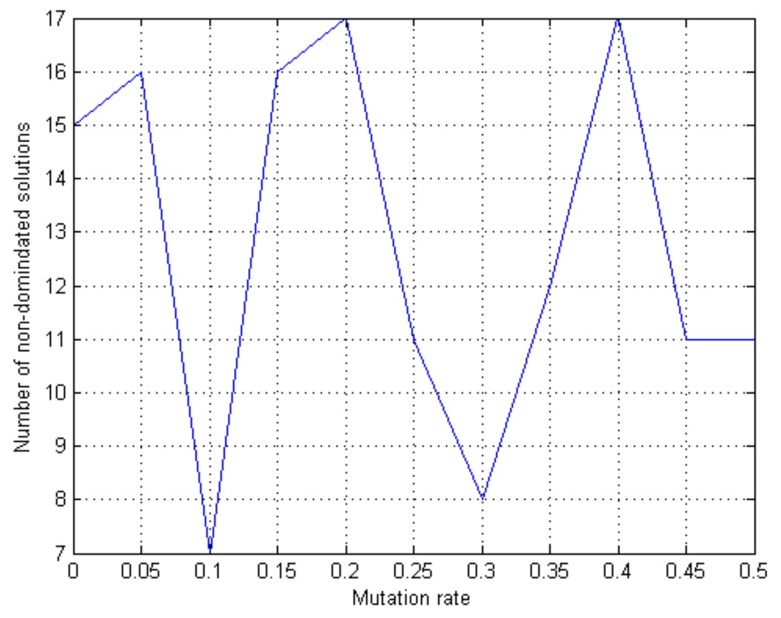
Figure 5.
Number of nondominated solutions vs. crossover rate.

Figure 6.
Number of nondominated solutions vs. population size.

Figure 7.
Percentage of individuals obtained.

Figure 8.
Percentage of individuals obtained by mutation by crossover.

Figure 9.
Curve of objective function 1.

Figure 10.
Curve of objective function 2.

Figure 11.
Pareto front solution set for using the NSGA-II to optimize the objective function.

Figure 12.
Distribution routes of deliverymen 1–7.
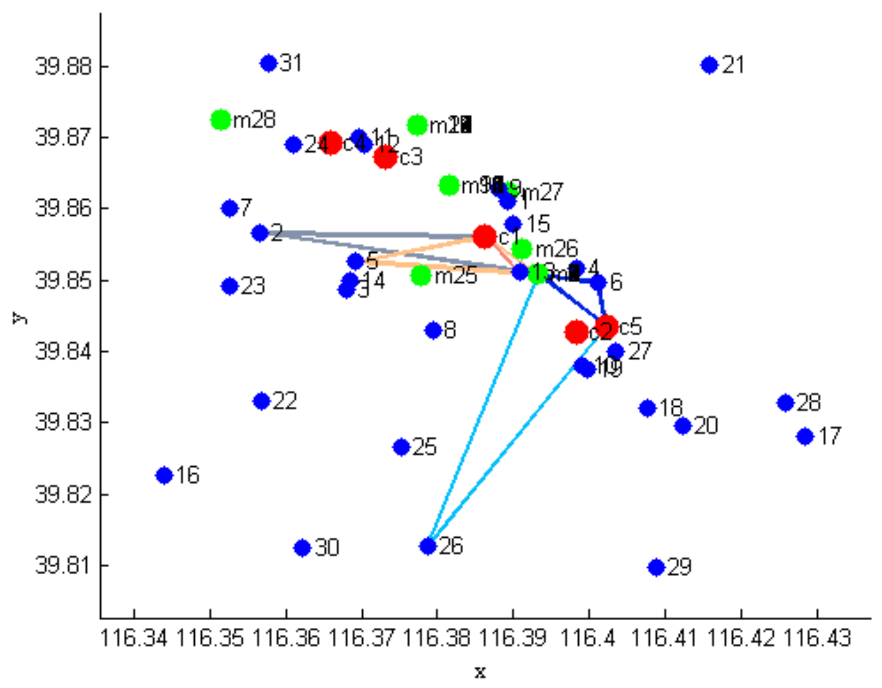
Figure 13.
Distribution routes of deliverymen 8–14.

Figure 14.
Distribution routes of deliverymen 15–21.

Figure 15.
Routes of deliverymen 22–28.


Table 1.
The status of some orders of merchant 1.
| Customer Number | Demand Quantity | Starting Time | Preparation Time (Min) | Longest Time (Min) |
|---|---|---|---|---|
| 1 | 1 | 12:04 | 2 | 30 |
| 2 | 1 | 12:03 | 10 | 45 |
| 5 | 1 | 12:32 | 5 | 45 |
| 8 | 1 | 12:47 | 10 | 60 |
| 12 | 1 | 12:56 | 5 | 45 |
| 16 | 1 | 12:34 | 5 | 45 |
In Table 1, the preparation time means the merchant’s goods preparation time before delivery, and the longest time means the longest time until the handover of goods.
Table 2.
The parameters used in the following simulations.
| Parameter | Value |
|---|---|
| Mutation rate | 0.2 |
| Crossover rate | 0.6 |
| Population size | 30 |
| Number of iterations | 2000 |
Table 3.
Routes obtained by using the NSGA-II.
| Deliveryman’s Number | Distribution Route | Deliveryman’s Number | Distribution Route |
|---|---|---|---|
| 1 | Merchant 1→13 | 15 | Merchant 1→8→Merchant 4→12→3 |
| 2 | Merchant 1→2 | 16 | Merchant 5→22→Merchant 3→21→24→Merchant 4→18 |
| 3 | Merchant 5→26 | 17 | Merchant 4→11→21 |
| 5 | Merchant 5→6 | 18 | Merchant 5→19→Merchant 2→3 |
| 7 | Merchant 1→5 | 20 | Merchant 5→28→Merchant 1→28 |
| 8 | Merchant 1→22→20 | 21 | Merchant 5→15→Merchant 1→1→12 |
| 9 | Merchant 3→10→Merchant 2→1 | 23 | Merchant 4→7→Merchant 2→26→16 |
| 10 | Merchant 2→6→11 | 24 | Merchant 3→19→17 |
| 11 | Merchant 3→14 | 25 | Merchant 2→9→Merchant 5→13 |
| 12 | Merchant 1→24→Merchant 4→2→Merchant 4→30→29→25 | 26 | Merchant 3→23 |
| 13 | Merchant 3→27→Merchant 2→19→7 | 28 | Merchant 3→4→Merchant 2→Merchant 1→18→16 |
Table 4.
Examples of order combination under multi-objective optimization.
| Distribution Route | Distance between Customers | Distribution Route | Distance between Vustomers |
|---|---|---|---|
| 18→16 | 5.55 km | 12→3 | 2.26 km |
| 29→25 | 3.42 km | 1→12 | 1.83 km |
Table 5.
Comparison of order dispatching and the combination between single-objective programming and multi-objective programming.
Table 5.
Comparison of order dispatching and the combination between single-objective programming and multi-objective programming.
| Model | Proportion of Deliverymen Dispatched | Average Number of Orders for Each Deliveryman |
|---|---|---|
| Single-Objective Programming | 67.9% | 2.58 |
| Multi-Objective Programming | 75.9% | 2.23 |
Table 6.
Comparisons of total cost, total mileage, and customer satisfaction between single-objective programming and multi-objective programming.
Table 6.
Comparisons of total cost, total mileage, and customer satisfaction between single-objective programming and multi-objective programming.
| Model | Total Cost | Total Mileage | Customer Satisfaction |
|---|---|---|---|
| Single-Objective Programming | 460.3 | 156.1 | NA |
| Multi-Objective Programming | 468.1 | 169.1 | 85.4% |
| RV | 1.017% | 1.083% | NA |
Table 7.
Comparison of delivery time efficiency between single-objective programming and multi-objective programming.
Table 7.
Comparison of delivery time efficiency between single-objective programming and multi-objective programming.
| Model | ER | LR |
|---|---|---|
| Single-Objective Programming | 57.14% | 87.76% |
| Multi-Objective Programming | 61.22% | 91.84% |
© 2020 by the authors. Licensee MDPI, Basel, Switzerland. This article is an open access article distributed under the terms and conditions of the Creative Commons Attribution (CC BY) license (http://creativecommons.org/licenses/by/4.0/).
Share and Cite
MDPI and ACS Style
Zhang, Y.; Yuan, C.; Wu, J. Vehicle Routing Optimization of Instant Distribution Routing Based on Customer Satisfaction. Information 2020, 11, 36. https://0-doi-org.brum.beds.ac.uk/10.3390/info11010036
AMA Style
Zhang Y, Yuan C, Wu J. Vehicle Routing Optimization of Instant Distribution Routing Based on Customer Satisfaction. Information. 2020; 11(1):36. https://0-doi-org.brum.beds.ac.uk/10.3390/info11010036
Chicago/Turabian StyleZhang, Yan, Chunhui Yuan, and Jiang Wu. 2020. "Vehicle Routing Optimization of Instant Distribution Routing Based on Customer Satisfaction" Information 11, no. 1: 36. https://0-doi-org.brum.beds.ac.uk/10.3390/info11010036
Note that from the first issue of 2016, this journal uses article numbers instead of page numbers. See further details here.