Recursive Matrix Calculation Paradigm by the Example of Structured Matrix

Abstract

In this paper, we derive recursive algorithms for calculating the determinant and inverse of the generalized Vandermonde matrix. The main advantage of the recursive algorithms is the fact that the computational complexity of the presented algorithm is better than calculating the determinant and the inverse by means of classical methods, developed for the general matrices. The results of this article do not require any symbolic calculations and, therefore, can be performed by a numerical algorithm implemented in a specialized (like Matlab or Mathematica) or general-purpose programming language (C, C++, Java, Pascal, Fortran, etc.).

1. Introduction

In previous studies [1,2], we proposed a classical numerical method for inverting the generalized Vandermonde matrix (GVM). The new contributions in this article are as follows:

• We derive recursive algorithms for calculating the determinant and inverse of the generalized Vandermonde matrix.
• The importance of the recursive algorithms becomes clear when we consider practical implementation of the GVM; they are useful each time we add a new interpolation node or a new root of a given differential equation in question.
• The recursive algorithms, which we propose in this work, can allow avoiding the recalculation of the determinant and/or inverse.
• The main advantage of the recursive algorithms is the fact that the computational complexity of the presented algorithm is of the O(n) class for the computation of the determinant.
• The results of this article do not require any symbolic calculations and, therefore, can be performed by a numerical algorithm implemented in a high-level (like Matlab or Mathematica) or low-level programming language (C, C++, Java, Pascal, Fortran, etc.).

In this article, we neatly combined the results from previous studies [3,4] and extended the computational examples.

The main results of this article are shown in Algorithms 1 and 2. The paper is organized as follows: Section 2 justifies the importance of the generalized Vandermonde matrices, Section 3 gives the recursive algorithms for the generalized Vandermonde matrix determinant, Section 4 gives two recursive algorithms for calculating the desired inverse, Section 5 presents, with an example, the application of the proposed algorithms, and Section 6 summarizes the article.

2. Practical Importance of the Generalized Vandermonde Matrix

In this article, we consider the generalized Vandermonde matrix (GVM) of the form proposed by El-Mikkawy [5]. The classical form is considered in References [6,7]. For the $n\in Z_{+}$ real pairwise distinct roots $c_1,\dots ,c_n$ and the real constant coefficient $k$, we define the GVM as follows:

$$V_G^{(k)}\left(c_1,\dots ,c_n\right)=\left[\begin{array}{cccc}{c}_1^k& c_1^{k+1}& \cdots & c_1^{k+n-1}\\ c_2^k& c_2^{k+1}& \cdots & c_2^{k+n-1}\\ ⋮& ⋮& \ddots & ⋮\\ c_n^k& c_n^{k+1}& \cdots & c_n^{k+n-1}\end{array}\right].$$

(1)

These matrices arise in a broad range of both theoretical and practical issues. Below, we survey the issues which require the use of the generalized Vandermonde matrices.

▪

Linear, ordinary differential equations (ODE): the Jordan canonical form matrix of the ODE in the Frobenius form is a generalized Vandermonde matrix ([8] pp. 86–95).

▪

Control issues: investigating the so-called controllability [9] of the higher-order systems leads to the issue of inverting the classic Vandermonde matrix [10] (in the case of distinct zeros of the system characteristic polynomial) and the generalized Vandermonde matrix [11] (for systems with multiple characteristic polynomial zeros). As the examples of the higher-order models of the physical objects, we can mention Timoshenko’s elastic beam equation [12] (fourth order) and Korteweg-de Vries’s equation of waves on shallow water surfaces [13,14] (third, fifth, and seventh order).

▪

Interpolation: apart from the ordinary polynomial interpolation with single nodes, we consider the Hermite interpolation, allowing multiple interpolation nodes. This issue leads to the system of linear equations, with the generalized Vandermonde matrix ([15] pp. 363–373).

▪

Information coding: the generalized Vandermonde matrix is used in coding and decoding information in the Hermitian code [16].

▪

Optimization of the non-homogeneous differential equation [17].

3. Algorithms for the Generalized Vandermonde Matrix Determinant

In this chapter, we propose a library of recursive algorithms for the calculation of the generalized Vandermonde matrix determinant. These algorithms solve the following set of practically important, incremental problems:

(A)

Suppose we have the value of the Vandermonde determinant for a given series of roots $c_1,\dots ,c_{n-1}$. How can we calculate the determinant after inserting another root into an arbitrary position in the root series, without the need to recalculate the whole determinant? This problem corresponds to the situation which frequently emerges in practice, i.e., adding a new node (polynomial interpolation) or increasing the order of the characteristic equation (linear differential equation solving, optimization, and control problems).

(B)

Contrary to the previous scenario, we have the Vandermonde determinant value for a given root series $c_1,\dots ,c_n$. We remove an arbitrary root $c_q$ from the series. How can we recursively calculate the determinant in this case? The examples of real applications from the previous point also apply here. The proper solution is given in Section 3.1.

(C)

We are searching for the determinant value, when, in the given root series $c_1,\dots ,c_n$, we change the value of an arbitrarily chosen root (Section 3.1).

(D)

We are searching for the determinant value, for the given root series $c_1,\dots ,c_n$, calculated recursively.

The theorem below is the main tool to construct the above recursive algorithm.

3.1. The Recursive Determinant Formula

Theorem 1.

The following recursive formula is fulfilled for the generalized Vandermonde matrix:

$$\det V_G^{(k)}\left(c_1,\dots ,c_n\right)={\left(-1\right)}^{q+1}{c}_q^k\cdot \det V_G^{(k)}\left(c_1,\dots ,c_{{}_{q-1}},c_{{}_{q+1}},\dots ,c_n\right)\cdot {\displaystyle \prod _{i=1,i\ne q}^n\left(c_i-c_q\right)},q=1,..,n.$$

(2)

Proof. 

Applying the standard determinant linear properties, we can obtain

$$\det V_G^{(k)}\left(c_1,\dots ,c_n\right)=\det \left[\begin{array}{cccc}{c}_1^k& c_1^{k+1}& \cdots & c_1^{k+n-1}\\ ⋮& ⋮& \ddots & ⋮\\ c_q^k& c_q^{k+1}& \cdots & c_q^{k+n-1}\\ ⋮& ⋮& \ddots & ⋮\\ c_n^k& c_n^{k+1}& ⋮& c_n^{k+n-1}\end{array}\right]=\det \left[\begin{array}{cccc}{c}_1^k& (c_1^k{c}_1-c_1^k{c}_q)& \cdots & (c_1^k{c}_1^{n-1}-c_1^k{c}_1^{n-2}{c}_q)\\ ⋮& ⋮& \ddots & ⋮\\ c_q^k& 0& \cdots & 0\\ ⋮& ⋮& \ddots & ⋮\\ c_n^k& (c_n^k{c}_n-c_n^k{c}_q)& ⋮& (c_n^k{c}_n^{n-1}-c_n^k{c}_n^{n-2}{c}_q)\end{array}\right].$$

Next, in compliance with Laplace’s expansion formula applied to the q-th column, we directly have

$$\begin{gathered} \det V_G^{(k)}\left(c_1,\dots ,c_n\right)={\left(-1\right)}^{q+1}{c}_q^k\det \left[\begin{array}{cccc}{c}_1^k\left(c_1-c_q\right)& c_1^{k+1}\left(c_1-c_q\right)& \cdots & c_1^{k+n-2}\left(c_1-c_q\right)\\ ⋮& ⋮& \ddots & ⋮\\ c_{q-1}^k\left(c_{q-1}-c_q\right)& c_{q-1}^{k+1}\left(c_{q-1}-c_q\right)& \cdots & c_{q-1}^{k+n-2}\left(c_{q-1}-c_q\right)\\ c_{q+1}^k\left(c_{q+1}-c_q\right)& c_{q+1}^{k+1}\left(c_{q+1}-c_q\right)& \cdots & c_{q+1}^{k+n-2}\left(c_{q+1}-c_q\right)\\ ⋮& ⋮& \ddots & ⋮\\ c_n^k\left(c_n-c_q\right)& c_n^{k+1}\left(c_n-c_q\right)& \cdots & c_n^{k+n-2}\left(c_n-c_q\right)\end{array}\right] \\ ={\left(-1\right)}^{q+1}{c}_q^k\det \left[\begin{array}{cccc}{c}_1^k& c_1^{k+1}& \cdots & c_1^{k+n-2}\\ ⋮& ⋮& \ddots & ⋮\\ c_{q-1}^k& c_{q-1}^{k+1}& \cdots & c_{q-1}^{k+n-2}\\ c_{q+1}^k& c_{q+1}^{k+1}& \cdots & c_{q+1}^{k+n-2}\\ ⋮& ⋮& \ddots & ⋮\\ c_n^k& c_n^{k+1}& \cdots & c_n^{k+n-2}\end{array}\right]\cdot {\displaystyle \prod _{\begin{array}{l}i=1\\ i\ne q\end{array}}^n\left(c_i-c_q\right)}. \end{gathered}$$

This concludes the proof of Equation (2).

Directly from Theorem 1, we can obtain the algorithms below for the incremental problems A–D. The detailed implementation of these formulas is straightforward and omitted.

Cases A, B: All we need to do is apply Equation (2).

Case C: Let us assume that, for the given root series $c_1,\dots ,c_n$, the corresponding determinant value is equal to $\det V_G^{(k)}\left(c_1,\dots ,c_q,\dots ,c_n\right)$. Our objective is to find the value of the determinant $\det V_G^{(k)}\left(c_1,\dots ,c_q^{}+\mathsf{\Delta }{c}_q,\dots ,c_n\right)$. Applying Equation (2) twice, we can obtain the following expression for the searched determinant:

$$\det V_G^{(k)}\left(c_1,\dots ,c_q^{}+\mathsf{\Delta }{c}_q,\dots ,c_n\right)={\left(\frac{c_q^{}+\mathsf{\Delta }{c}_q}{c_q}\right)}^k\frac{{\displaystyle \prod _{i=1,i\ne q}^n\left(c_i-c_q^{}-\mathsf{\Delta }{c}_q\right)}}{{\displaystyle \prod _{i=1,i\ne q}^n\left(c_i-c_q\right)}}\det V_G^{(k)}\left(c_1,\dots ,c_q,\dots ,c_n\right),q=1,..,n.$$

Case D: The proper recursive function expressing the determinant value, for the given root series $c_1,\dots ,c_n$, has the following form:

$$\det V_G^{(k)}\left(c_1,\dots ,c_q\right)=\{\begin{array}{cc}{\left(-1\right)}^{q+1}{c}_q^k\cdot \det V_G^{(k)}\left(c_1,\dots ,c_{{}_{q-1}}\right){\displaystyle \prod _{i=1}^{q-1}\left(c_i-c_q\right)},\hfill & \mathrm{for}q>1\hfill \\ {\mathrm{c}}_1^{\mathrm{k}},\hfill & \mathrm{for}q=1\hfill \end{array}.$$

 ☐

3.2. Computational Complexity of the Proposed Algorithms

The following facts are worth noting:

▪

The computational complexity of the presented Algorithms A–C is of the O(n) class with respect to the number of floating-point operations necessary to perform. This enables us to efficiently solve the incremental Vandermonde problems, avoiding the quadratic complexity, typical in the Vandermonde field (e.g., References [14,18])

▪

Algorithm D is of the O(n²) class, being, by the linear term, more efficient than the ordinary Gauss elimination method.

3.3. Special Cases

In this section, we give special forms of Algorithms A–D tuned for two special cases of the generalized Vandermonde matrix, i.e., for the equidistant roots, as well as the roots equal to the succeeding positive integers.

3.3.1. Generalized Vandermonde Matrix with Equidistant Roots

Let us take into account the GVM with the equidistant roots of the form $c_i=c_1+(i-1)h,h\in R$. In this special case Formula (2) becomes

$$\det V_G^{(k)}\left(c_1,\dots ,c_n\right)=\left(q-1\right)!\left(n-q\right)!h^{n-1}{c}_q^k\det V_G^{(k)}\left(c_1,\dots ,c_{{}_{q-1}},c_{{}_{q+1}},\dots ,c_n\right),q=1,..,n,$$

(3)

and Algorithms A–D change to the recursive Equation (3).

3.3.2. Generalized Vandermonde Matrix with Positive Integer Roots

In Reference [5], it is considered a special case of GVM, which can be obtained from Equation (1) when $c_i=i,i=1,\dots ,n$, denoting this matrix by $V_S^{(k)}(n)$.

$$V_S^{(k)}\left(1,\dots ,n\right)=\left[\begin{array}{cccc}1& 1& \cdots & 1\\ 2^k& 2_{}^{k+1}& \cdots & 2_{}^{k+n-1}\\ ⋮& ⋮& \ddots & ⋮\\ n_{}^k& n_{}^{k+1}& \cdots & n_{}^{k+n-1}\end{array}\right].$$

(4)

For the special $V_S^{(k)}$, Equation (3) becomes

$$\det V_S^{(k)}\left(1,\dots ,n\right)=\left(q-1\right)!\left(n-q\right)!c_q^k\det V_S^{(k)}\left(1,\dots ,q-1,q+1,\dots ,n\right),q=1,..,n.$$

(5)

4. Algorithms for the Generalized Vandermonde Matrix Inverse

In this chapter, we give a recursive algorithm to invert the generalized Vandermonde matrix of Equation (1). At first, let us refer to the known, non-recursive results within this topic presented previously [5]. Reference [5] features an explicit form of the GVM inverse, which makes use of the so-called elementary symmetric functions, defined below.

4.1. Definition of the Elementary Symmetric Functions

If the $n$ parameters $c_1,c_2,\dots ,c_n$ are distinct, then the elementary symmetric functions ${\sigma }_{i,j}^{(n)}$ in $c_1,c_2,\dots ,c_{j-1},c_{j+1},\dots ,c_n$ are defined for $i,j=1,\dots ,n$ in El-Mikkawy [5] p. 644 by

$$\{\begin{array}{l}{\sigma }_{1,j}^{(n)}=1\\ {\sigma }_{i,j}^{(n)}={\displaystyle \sum _{\begin{array}{l}{r}_1=1\\ r_1\ne j\end{array}}^n}{\displaystyle \sum _{\begin{array}{l}{r}_2=r_1+1\\ r_2\ne j\end{array}}^n\dots }{\displaystyle \sum _{\begin{array}{l}{r}_{i-1}=r_{i-2}+1\\ r_{i-1}\ne j\end{array}}^n}{\displaystyle \prod _{m=1}^{i-1}{c}_{r_m}},\hspace{1em}fori=2,\dots ,n\end{array}.$$

(6)

The efficient algorithm, of the O(n²) computational complexity class, for calculating the elementary symmetric functions in Equation (6), is given in Reference [5]. Now, it is possible to present the explicit form of the inverse GVM given by Reference [5] (p. 647).

$${\left[V_G^{(k)}\left(1,\dots ,n\right)\right]}^{-1}=\left[\begin{array}{cccc}\frac{{(-1)}^{n+1}{\sigma }_{n,1}^{(n)}}{c_1^k{\displaystyle \prod _{i=2}^n(c_1-c_i)}}& \frac{{(-1)}^{n+1}{\sigma }_{n,2}^{(n)}}{c_2^k{\displaystyle \prod _{i=1,i\ne 2}^n(c_2-c_i)}}& \cdots & \frac{{(-1)}^{n+1}{\sigma }_{n,n}^{(n)}}{c_n^k{\displaystyle \prod _{i=1}^{n-1}(c_n-c_i)}}\\ \frac{{(-1)}^{n+2}{\sigma }_{n-1,1}^{(n)}}{c_1^k{\displaystyle \prod _{i=2}^n(c_1-c_i)}}& \frac{{(-1)}^{n+2}{\sigma }_{n-1,2}^{(n)}}{c_2^k{\displaystyle \prod _{i=1,i\ne 2}^n(c_2-c_i)}}& \cdots & \frac{{(-1)}^{n+2}{\sigma }_{n-1,n}^{(n)}}{c_n^k{\displaystyle \prod _{i=1}^{n-1}(c_n-c_i)}}\\ ⋮& ⋮& \ddots & ⋮\\ \frac{{(-1)}^{n+n}{\sigma }_{1,1}^{(n)}}{c_1^k{\displaystyle \prod _{i=2}^{n-1}(c_1-c_i)}}& \frac{{(-1)}^{n+n}{\sigma }_{1,2}^{(n)}}{c_2^k{\displaystyle \prod _{i=1,i\ne 2}^{n-1}(c_2-c_i)}}& \cdots & \frac{{(-1)}^{n+n}{\sigma }_{1,n}^{(n)}}{c_n^k{\displaystyle \prod _{i=1}^{n-1}(c_n-c_i)}}\end{array}\right].$$

(7)

Let us return to the objective of this chapter, i.e., construction of the efficient, recursive algorithm for inverting the generalized Vandermonde matrix. This issue can be formalized as follows: we know the GVM inverse for the root series $c_1,\dots ,c_n$. We want to efficiently calculate the inverse for the root series $c_1,\dots ,c_n,c_{n+1}$, making use of the known inverse. Let $V_G^{(k)}\left(n+1\right)=V_G^{(k)}\left(c_1,c_2,\dots ,c_{n+1}\right)$; then, the theorem below enables recursively calculating the desired inverse.

4.2. Theorem of the Recursive Inverse

Theorem 2.

The inverse generalized Vandermonde matrix ${\left[V_G^{(k)}\left(n+1\right)\right]}^{-1}$, corresponding to the root series $c_1,\dots ,c_{n+1}$, can be expressed by the following block matrix:

$${\left[V_G^{(k)}\left(n+1\right)\right]}^{-1}=\left[\begin{array}{cc}{\left[V_G^{(k)}\left(n\right)\right]}^{-1}+\frac{{\left[V_G^{(k)}\left(n\right)\right]}^{-1}\left[\begin{array}{c}{c}_1^{k+n}\\ ⋮\\ c_n^{k+n}\end{array}\right]\left[\begin{array}{ccc}{c}_{n+1}^k& \cdots & c_{n+1}^{k+n-1}\end{array}\right]{\left[V_G^{(k)}\left(n\right)\right]}^{-1}}{d}& -\frac{{\left[V_G^{(k)}\left(n\right)\right]}^{-1}\left[\begin{array}{c}{c}_1^{k+n}\\ ⋮\\ c_n^{k+n}\end{array}\right]}{d}\\ -\frac{\left[\begin{array}{ccc}{c}_{n+1}^k& \cdots & c_{n+1}^{k+n-1}\end{array}\right]{\left[V_G^{(k)}\left(n\right)\right]}^{-1}}{d}& \frac{1}{d}\end{array}\right],$$

(8)

$$d=c_{n+1}^{k+n}-\left[\begin{array}{ccc}{c}_{n+1}^k& \cdots & c_{n+1}^{k+n-1}\end{array}\right]{\left[V_G^{(k)}\left(n\right)\right]}^{-1}\left[\begin{array}{c}{c}_1^{k+n}\\ ⋮\\ c_n^{k+n}\end{array}\right],$$

(9)

where ${\left[V_G^{(k)}\left(n\right)\right]}^{-1}$ denotes the known GVM inverse for the roots $c_1,\dots ,c_n$.

Proof. 

To prove the matrix recursive identity in Equation (8), we make use of the block matrix algebra rules. A useful formula, expressing the block matrix inverse by the inverses of the respective sub-matrices, is:

$$A^{-1}={\left[\begin{array}{cc}{A}_1& A_2\\ A_3& A_4\end{array}\right]}^{-1}=\left[\begin{array}{cc}{A}_1^{-1}+A_1^{-1}{A}_2{B}^{-1}{A}_3{A}_1^{-1}& -A_1^{-1}{A}_2{B}^{-1}\\ -B^{-1}{A}_3{A}_1^{-1}& B^{-1}\end{array}\right],\hspace{1em}B=A_4-A_3{A}_1^{-1}{A}_2.$$

(10)

Thus, if we know the inverse of the sub-matrix $A_1$ and the inverse of $B$, we can directly obtain the inverse of the block matrix $A$ by performing a few matrix multiplications. For different $c_1,c_2,\dots ,c_{n+1}$, the GVM matrix is invertible and Equation (10) holds true; thus, the coefficient $d$ given by Equation (9) is non-zero. Now, let us take into account the generalized Vandermonde matrix $V_G^{(k)}\left(n+1\right)$ for the $n+1$ roots $c_1,\dots ,c_{n+1}$. It can be treated as a block matrix of the following form:

$$V_G^{(k)}\left(n+1\right)=\left[\begin{array}{cccc}{c}_1^k& \cdots & c_1^{k+n-1}& c_1^{k+n}\\ ⋮& \ddots & ⋮& ⋮\\ c_n^k& \cdots & c_n^{k+n-1}& c_n^{k+n}\\ c_{n+1}^k& \cdots & c_{n+1}^{k+n-1}& c_{n+1}^{k+n}\end{array}\right]=\left[\begin{array}{cc}\left[V_G^{(k)}\left(n\right)\right]& \left[\begin{array}{c}{c}_1^{k+n}\\ ⋮\\ c_n^{k+n}\end{array}\right]\\ \left[\begin{array}{ccc}{c}_{n+1}^k& \cdots & c_{n+1}^{k+n-1}\end{array}\right]& \left[c_{n+1}^{k+n}\right]\end{array}\right].$$

(11)

Now, applying the block matrix identities in Equation (10) to the block matrix in Equation (11), we directly obtain the thesis in Equation (9).

Despite the explicit form of the block matrix inverse in Equation (9), its efficient algorithmic implementation is not obvious. The order in which we calculate the matrix term ${\left[V_G^{(k)}\left(n\right)\right]}^{-1}{\left[\begin{array}{ccc}{c}_1^{k+n}& \cdots & c_n^{k+n}\end{array}\right]}^T\left[\begin{array}{ccc}{c}_{n+1}^k& \cdots & c_{n+1}^{k+n-1}\end{array}\right]{\left[V_G^{(k)}\left(n\right)\right]}^{-1}$ has a crucial influence on the final computational complexity of the algorithm. Therefore, let us analyze all three possible orders.

(A) Left-to-right order of multiplications.

One can notice that ${\left[V_G^{(k)}\left(n\right)\right]}^{-1}{\left[\begin{array}{ccc}{c}_1^{k+n}& \cdots & c_n^{k+n}\end{array}\right]}^T\left[\begin{array}{ccc}{c}_{n+1}^k& \cdots & c_{n+1}^{k+n-1}\end{array}\right]$ has dimensions equal to $\mathrm{n}\times \mathrm{n}$. Hence, the multiplication of this last matrix and of the matrix ${\left[V_G^{(k)}\left(n\right)\right]}^{-1}$ is an O(n³) class algorithm. Thus, the computational complexity in the left-to-right order is of the O(n³) class.

(B) Right-to-left order.

A detailed analysis leads also to the O(n³) class.

(C) The order of the following form:

$$\left\{{\left[V_G^{(k)}\left(n\right)\right]}^{-1}{\left[\begin{array}{ccc}{c}_1^{k+n}& \cdots & c_n^{k+n}\end{array}\right]}^T\right\}\left\{\left[\begin{array}{ccc}{c}_{n+1}^k& \cdots & c_{n+1}^{k+n-1}\end{array}\right]{\left[V_G^{(k)}\left(n\right)\right]}^{-1}\right\}.$$

(12)

In this case, at first, we perform the following two multiplications:

• The multiplication $\left\{{\left[V_G^{(k)}\left(n\right)\right]}^{-1}{\left[\begin{array}{ccc}{c}_1^{k+n}& \cdots & c_n^{k+n}\end{array}\right]}^T\right\}$ requires O(n²) operations; as the result, we get the n-element vertical vector.
• The multiplication $\left\{\left[\begin{array}{ccc}{c}_{n+1}^k& \cdots & c_{n+1}^{k+n-1}\end{array}\right]{\left[V_G^{(k)}\left(n\right)\right]}^{-1}\right\}$ requires O(n²) operations; as the result, we get the n-element horizontal vector.  ☐

Finally, all we have to do is to multiply these two last vectors, which obviously is an operation of the O(n²) class.

Summarizing, the most efficient is the multiplication order ((C), giving a quadratic computational complexity. All other orders lead to the worse O(n³) class algorithms. Combining the above results, we can give the algorithm which solves the incremental inverse problem, i.e., calculating the GVM inverse for the root series $c_1,\dots ,c_n,c_{n+1}$ on the basis of the known inverse for the root series $c_1,\dots ,c_n$.

4.3. Algorithm 1

Using the incremental Algorithm 1, we can build the final, recursive algorithm for inverting the generalized Vandermonde matrix of the form in Equation (1).

Algorithm 1:Incremental Inverting of the Generalized Vandermonde Matrix

1.  Function Incremental_Inverse(n; k; $c_1,\dots ,c_{n+1}$; ${\left[V_G^{(k)}\left(n\right)\right]}^{-1}$): ${\left[V_G^{(k)}\left(n+1\right)\right]}^{-1}$ 2.  Input: - $n\hspace{1em}\hspace{1em}\hspace{1em}\hspace{1em}\hspace{1em}:integer$  -number of roots − 1 - $k\hspace{1em}\hspace{1em}\hspace{1em}\hspace{1em}\hspace{1em}:real$    -Vandermonde matrix general exponent - $c_1,\dots ,c_{n+1}\hspace{1em}:real$     -the roots - ${\left[V_G^{(k)}\left(n\right)\right]}^{-1}:rea{l}^{n\times n}$    -the GVM inverse for the roots $c_1,\dots ,c_n$. 3.  Locals: - ${\overline{v}}_1,{\overline{v}}_2:rea{l}^n$ - $d:real$ 4.  Calculate the auxiliary vectors ${\overline{v}}_1,{\overline{v}}_2$. $${\overline{v}}_1:={\left[V_G^{(k)}\left(n\right)\right]}^{-1}{\left[\begin{array}{ccc}{c}_1^{k+n}& \cdots & c_n^{k+n}\end{array}\right]}^T.$$ (13) $${\overline{v}}_2:=\left[\begin{array}{ccc}{c}_{n+1}^k& \cdots & c_{n+1}^{k+n-1}\end{array}\right]{\left[V_G^{(k)}\left(n\right)\right]}^{-1}.$$ (14) 5.  Calculate the coefficient $d$ using Equation (9). $$d:=c_{n+1}^{k+n}-{\overline{v}}_2{\left[\begin{array}{ccc}{c}_1^{k+n}& \cdots & c_n^{k+n}\end{array}\right]}^T.$$ (15) 6.  Build the desired matrix inverse ${\left[V_G^{(k)}\left(n+1\right)\right]}^{-1}$ as a block matrix. $${\left[V_G^{(k)}\left(n+1\right)\right]}^{-1}:=\left[\begin{array}{cc}{\left[V_G^{(k)}\left(n\right)\right]}^{-1}+\frac{{\overline{v}}_1{\overline{v}}_2}{d}& -\frac{{\overline{v}}_1}{d}\\ -\frac{{\overline{v}}_2}{d}& \frac{1}{d}\end{array}\right].$$ (16) 7.  Output: - ${\left[V_G^{(k)}\left(n+1\right)\right]}^{-1}:rea{l}^{(n+1)\times (n+1)}$-the inverse for the roots $c_1,\dots ,c_n,c_{n+1}$. 8.  End.

4.4. Computational Complexity

It is possible to note the following advantages of the computational complexity of inverting the GVM by recursive algorithms in comparison with the classical Equation (7), the complexity of which is O(n³) (the classical Equation (7) requires calculating the elementary symmetric functions ${\sigma }_{i,j}^{(n)}$ for $i,j=1,\dots ,n$. To this aim, Algorithm 2.1 p. 644 [5], with quadratic complexity, should be executed n times (Formula 2.5, p. 645):

▪

As we analyzed in the point (C), Section 4.2, the computational complexity of the incremental Algorithm 1, which is constructed on the basis of of Equation (12), is of the O(n²) class with respect to the number of floating-point operations which have to be performed. This is possible thanks to the proper multiplication order in Equation (12). This way, we avoid the O(n³) complexity while adding a new root.

▪

The computational complexity of the recursive Algorithm 2 is of the O(n³) class.

Algorithm 2:For Recursive Inverting the Generalized Vandermonde Matrix.

1.  Function Inverse(n; k; $c_1,\dots ,c_n$): ${\left[V_G^{(k)}\left(n\right)\right]}^{-1}$ 2.  Input: - $n\hspace{1em}\hspace{1em}\hspace{1em}\hspace{1em}:integer$  - number of roots - $k\hspace{1em}\hspace{1em}\hspace{1em}\hspace{1em}:real$    - Vandermonde matrix general exponent - $c_1,\dots ,c_n\hspace{1em}:real$    -the roots 3.  Locals: - $V[][]ofreal$ - $i\text{:}\mathit{integer}$ 4.  Calculate the variable V: V = $\frac{1}{{\mathrm{c}}_1^{\mathrm{k}}}$ 5.  For i = 1 To n − 1 V = Incremental_Inverse(i,k,$c_1,\dots ,c_{i+1}$,V) Next i 6.  Output: - $V:rea{l}^{n\times n}$ - the inverse for the roots $c_1,\dots ,c_n$. 7.  End.

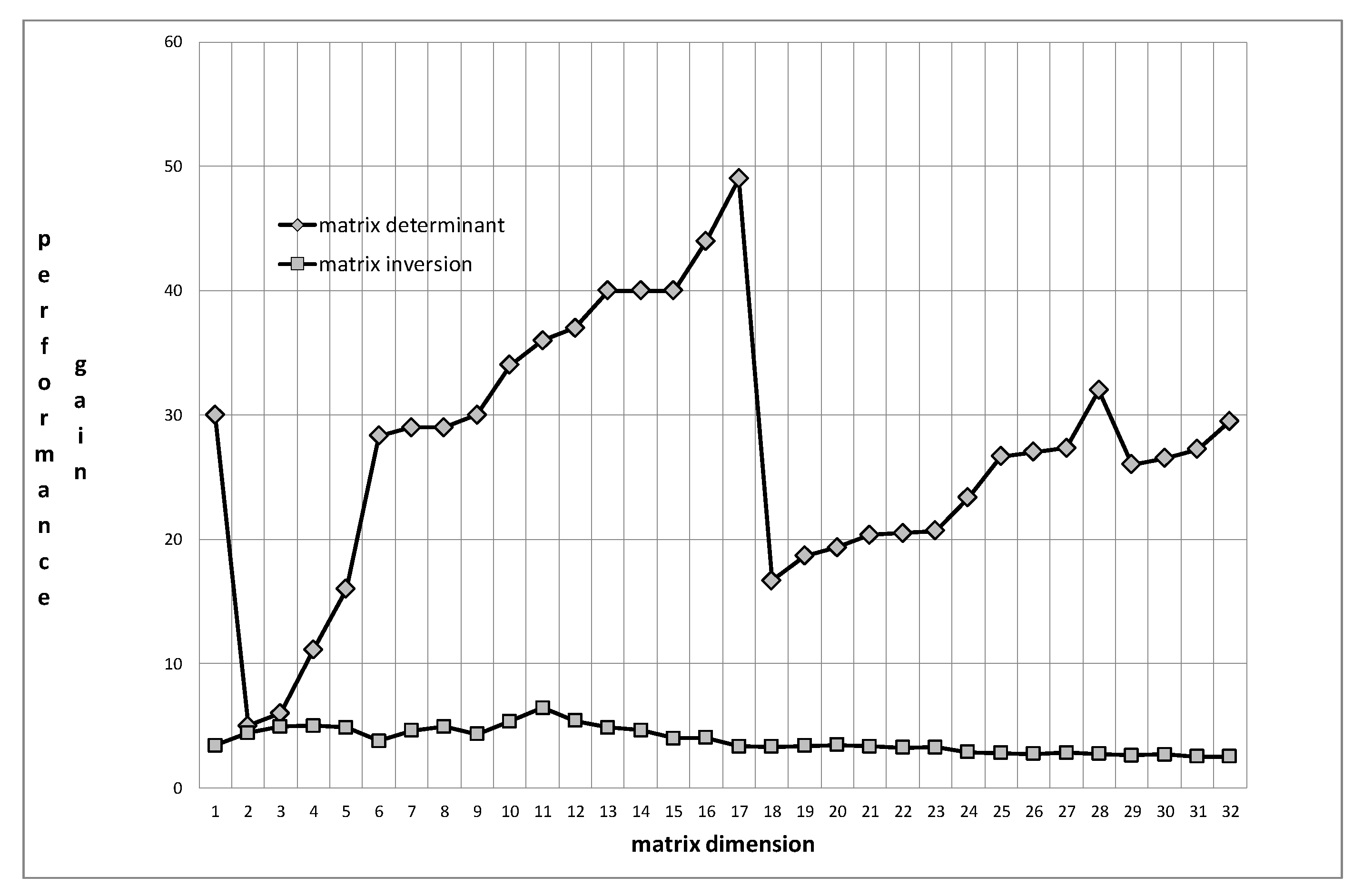
Last but not least, Equation (7) requires recalculating the desired inverse each time we add a new root. The main idea of the recursive algorithms we proposed is to make use of the already calculated inverse. This is how high efficiency was obtained. On the graphs below, we practically compare the efficiency of the recursive algorithms with the standard algorithms (in a non-recursive form, for matrices with arbitrary entries, contrary to the algorithms presented in this article, which are developed specially for the GVM) embedded in Matlab^®. On the left, we can see the execution time of the standard and recursive algorithms, and, on the right, we can see the relative performance gain (recursive algorithms vs. the standard ones for inversion and determinant calculation).

On Figure 1 and Figure 2 we show a practical performance tests of the Algorithms 1 and 2.

5. Example

We show a practical application of the algorithms from this article using the same numerical example as in Reference [5] (p. 649), to enable easy comparison of the two opposite algorithms: classical and recursive. Let us consider the generalized Vandermonde matrix $V_G^{(k)}\left(n\right)$ and its inverse ${\left[V_G^{(k)}\left(n\right)\right]}^{-1}$ with the following parameters:

-

general exponent: $k=0.5$.

-

size: $n=7$.

-

roots: $c_i=i,i=1,\dots ,7$.

The generalized Vandermonde matrix of such parameters has the following form:

$$V_G^{(0.5)}\left(7\right)=\left[\begin{array}{ccccccc}1& 1& 1& 1& 1& 1& 1\\ \sqrt{2}& 2\sqrt{2}& 4\sqrt{2}& 8\sqrt{2}& 16\sqrt{2}& 32\sqrt{2}& 64\sqrt{2}\\ \sqrt{3}& 3\sqrt{3}& 9\sqrt{3}& 27\sqrt{3}& 81\sqrt{3}& 243\sqrt{3}& 729\sqrt{3}\\ 2& 8& 32& 128& 512& 2048& 8192\\ \sqrt{5}& 5\sqrt{5}& 25\sqrt{5}& 125\sqrt{5}& 625\sqrt{5}& 3125\sqrt{5}& 15625\sqrt{5}\\ \sqrt{6}& 6\sqrt{6}& 36\sqrt{6}& 216\sqrt{6}& 1296\sqrt{6}& 7776\sqrt{6}& 46656\sqrt{6}\\ \sqrt{7}& 7\sqrt{7}& 49\sqrt{7}& 343\sqrt{7}& 2401\sqrt{7}& 16807\sqrt{7}& 117649\sqrt{7}\end{array}\right].$$

(17)

The determinant of the matrix $V_G^{(0.5)}\left(7\right)$ and its inverse have the following forms, respectively:

$$\det \left[V_G^{(0.5)}\left(7\right)\right]=298598400\sqrt{35},$$

(18)

$${\left[V_G^{(0.5)}\left(7\right)\right]}^{-1}=\left[\begin{array}{ccccccc}7& \frac{-21}{\sqrt{2}}& \frac{35}{\sqrt{3}}& \frac{-35}{2}& \frac{21}{\sqrt{5}}& \frac{-7}{\sqrt{6}}& \frac{1}{\sqrt{7}}\\ \frac{-223}{20}& \frac{879}{20\sqrt{2}}& \frac{-949}{12\sqrt{3}}& 41& \frac{-201}{4\sqrt{5}}& \frac{1019}{60\sqrt{6}}& \frac{-7\sqrt{7}}{20}\\ \frac{319}{45}& \frac{-3929}{120\sqrt{2}}& \frac{389}{6\sqrt{3}}& \frac{-2545}{72}& \frac{134}{3\sqrt{5}}& \frac{-1849}{120\sqrt{6}}& \frac{29\sqrt{7}}{90}\\ \frac{-37}{16}& \frac{71}{6\sqrt{2}}& \frac{-1219}{48\sqrt{3}}& \frac{44}{3}& \frac{-185\sqrt{5}}{48}& \frac{41}{6\sqrt{6}}& \frac{-7\sqrt{7}}{48}\\ \frac{59}{144}& \frac{-9}{4\sqrt{2}}& \frac{247}{48\sqrt{3}}& \frac{-113}{36}& \frac{69}{16\sqrt{5}}& \frac{-19}{12\sqrt{6}}& \frac{5\sqrt{7}}{144}\\ \frac{-3}{80}& \frac{13}{60\sqrt{2}}& \frac{-25}{48\sqrt{3}}& \frac{1}{3}& \frac{-23}{48\sqrt{5}}& \frac{11}{60\sqrt{6}}& \frac{-\sqrt{7}}{240}\\ \frac{1}{720}& \frac{-1}{120\sqrt{2}}& \frac{1}{48\sqrt{3}}& \frac{-1}{72}& \frac{1}{48\sqrt{5}}& \frac{-1}{120\sqrt{6}}& \frac{1}{720\sqrt{7}}\end{array}\right].$$

(19)

5.1. Objective

Our objective is to find the determinant and inverse of the generalized Vandermonde matrix $V_G^{(0.5)}\left(8\right)$, with roots $c_i=i,i=1,\dots ,8$, in the recursive way.

5.2. Recursive Determinant Calculation

We calculate the determinant value of the matrix $V_G^{(0.5)}\left(8\right)$ using Equation (5) because the GVM in question has consecutive integer roots. In this case, the equality in Equation (5) leads to the following determinant value:

$$\det V_G^{(0.5)}\left(8\right)=\left(8-1\right)!\left(8-8\right)!\sqrt{8}\det V_G^{(0.5)}\left(7\right)=7!\sqrt{8}\cdot 298598400\sqrt{35}=3009871872000\sqrt{70}.$$

5.3. Recursive Inverse Finding

The task of calculating the inverse of the matrix $V_G^{(0.5)}\left(8\right)$ is performed using Algorithm 1, with the use of the known inverse ${\left[V_G^{(0.5)}\left(7\right)\right]}^{-1}$ in Equation (19). The auxiliary vectors ${\overline{v}}_1,{\overline{v}}_2$ have forms in compliance with Equations (13) and (14)

$$\begin{array}{ll}{\overline{v}}_1& ={\left[V_G^{(k)}\left(n\right)\right]}^{-1}{\left[\begin{array}{ccc}{c}_1^{k+n}& \cdots & c_n^{k+n}\end{array}\right]}^T={\left[V_G^{(k)}\left(n\right)\right]}^{-1}\sqrt{2}{\left[\begin{array}{ccccccc}2& 16& 128& 1024& 8192& 65536& 524288\end{array}\right]}^T=\\ & ={\left[\begin{array}{ccccccc}5040& -13068& 13132& -6769& 1960& -322& 28\end{array}\right]}^T\end{array}.$$

(20)

$$\begin{array}{ll}{\overline{v}}_2& =\left[\begin{array}{ccc}{c}_{n+1}^k& \cdots & c_{n+1}^{k+n-1}\end{array}\right]{\left[V_G^{(k)}\left(n\right)\right]}^{-1}=\left[\begin{array}{ccccccc}1& 128\sqrt{2}& 2187\sqrt{3}& 32768& 78125\sqrt{5}& 279936\sqrt{6}& 823543\sqrt{7}\end{array}\right]{\left[V_G^{(k)}\left(n\right)\right]}^{-1}=\\ & =\left[\begin{array}{ccccccc}2\sqrt{2}& -14& 14\sqrt{6}& -35\sqrt{2}& 14\sqrt{10}& -14\sqrt{3}& 2\sqrt{14}\end{array}\right]\end{array}.$$

(21)

Next, we calculate the coefficient $d$ as follows:

$$\begin{array}{ll}d=& c_{n+1}^{k+n}-{\overline{v}}_2{\left[\begin{array}{ccc}{c}_1^{k+n}& \cdots & c_n^{k+n}\end{array}\right]}^T=8^{7+0.5}-\left[\begin{array}{ccccccc}2\sqrt{2}& -14& 14\sqrt{6}& -35\sqrt{2}& 14\sqrt{10}& -14\sqrt{3}& 2\sqrt{14}\end{array}\right]\cdot \\ & \sqrt{2}{\left[\begin{array}{ccccccc}2& 16& 128& 1024& 8192& 65536& 524288\end{array}\right]}^T=\frac{1}{10080\sqrt{2}}\end{array}.$$

(22)

The last step of Algorithm 1 is building a block matrix in compliance with Equation (16). Combining the vectors ${\overline{v}}_1$ in Equation (20) and ${\overline{v}}_2$ in Equation (21), and the coefficient $d$ in Equation (22) with the known Vandermonde inverse ${\left[V_G^{(0.5)}\left(7\right)\right]}^{-1}$ in Equation (19), we finally obtain

$$\begin{array}{l}{\left[V_G^{(0.5)}\left(8\right)\right]}^{-1}=\left[\begin{array}{cc}{\left[V_G^{(0.5)}\left(7\right)\right]}^{-1}+\frac{{\overline{v}}_1{\overline{v}}_2}{d}& -\frac{{\overline{v}}_1}{d}\\ -\frac{{\overline{v}}_2}{d}& \frac{1}{d}\end{array}\right]\\ \hspace{0.17em}\hspace{0.17em}\hspace{0.17em}\hspace{0.17em}\hspace{0.17em}\hspace{0.17em}\hspace{0.17em}=\left[\begin{array}{cc}\begin{array}{ccccccc}8& -14\sqrt{2}& \frac{56}{3}\sqrt{3}& -35& \frac{56}{5}\sqrt{5}& \frac{-14}{3}\sqrt{6}& \frac{8}{7}\sqrt{7}\\ \frac{-481}{35}& \frac{621}{20}\sqrt{2}& \frac{-2003}{45}\sqrt{3}& \frac{691}{8}& \frac{-141}{5}\sqrt{5}& \frac{2143}{180}\sqrt{6}& \frac{-103}{35}\sqrt{7}\\ \frac{349}{36}& \frac{-18353}{720}\sqrt{2}& \frac{797}{20}\sqrt{3}& \frac{-1457}{18}& \frac{4891}{180}\sqrt{5}& \frac{-187}{16}\sqrt{6}& \frac{527}{180}\sqrt{7}\\ \frac{-329}{90}& \frac{15289}{1440}\sqrt{2}& \frac{-268}{15}\sqrt{3}& \frac{10993}{288}& \frac{-1193}{90}\sqrt{5}& \frac{2803}{480}\sqrt{6}& \frac{-67}{45}\sqrt{7}\\ \frac{115}{144}& \frac{-179}{72}\sqrt{2}& \frac{71}{16}\sqrt{3}& \frac{-179}{18}& \frac{2581}{720}\sqrt{5}& \frac{-13}{8}\sqrt{6}& \frac{61}{144}\sqrt{7}\\ \frac{-73}{720}& \frac{239}{720}\sqrt{2}& \frac{-149}{240}\sqrt{3}& \frac{209}{144}& \frac{-391}{720}\sqrt{5}& \frac{61}{240}\sqrt{6}& \frac{-49}{720}\sqrt{7}\\ \frac{1}{144}& \frac{-17}{720}\sqrt{2}& \frac{11}{240}\sqrt{3}& \frac{-1}{9}& \frac{31}{720}\sqrt{5}& \frac{-1}{48}\sqrt{6}& \frac{29}{5040}\sqrt{7}\end{array}& \begin{array}{c}\frac{-1}{4}\sqrt{2}\\ \frac{363}{560}\sqrt{2}\\ \frac{-469}{720}\sqrt{2}\\ \frac{967}{2880}\sqrt{2}\\ \frac{-7}{72}\sqrt{2}\\ \frac{23}{1440}\sqrt{2}\\ \frac{-1}{720}\sqrt{2}\end{array}\\ \begin{array}{ccccccc}\hspace{0.17em}\hspace{0.17em}\hspace{0.17em}\hspace{1em}\frac{-1}{5040}& \frac{1}{1440}\sqrt{2}\hspace{0.17em}\hspace{0.17em}\hspace{0.17em}\hspace{0.17em}& \frac{-1}{720}\sqrt{3}\hspace{0.17em}\hspace{0.17em}\hspace{0.17em}\hspace{0.17em}& \frac{1}{288}\hspace{0.17em}\hspace{0.17em}\hspace{0.17em}\hspace{0.17em}& \frac{-1}{720}\sqrt{5}\hspace{0.17em}\hspace{0.17em}\hspace{0.17em}\hspace{0.17em}& \frac{1}{1440}\sqrt{6}\hspace{0.17em}\hspace{0.17em}\hspace{0.17em}\hspace{0.17em}& \frac{-1}{5040}\sqrt{7}\end{array}& \frac{1}{20160}\sqrt{2}\end{array}\right]\end{array}$$

(23)

One can see that the incrementally received inverse ${\left[V_G^{(0.5)}\left(8\right)\right]}^{-1}$ is equivalent to the inverse obtained by the classical algorithms in Reference [5] (p. 649).

5.4. Summary of the Example

In this example, we recursively calculated the determinant and inverse of the $V_G^{(0.5)}\left(8\right)$ matrix, making use of the known determinant and the inverse of the $V_G^{(0.5)}\left(7\right)$ matrix, respectively. It is worth noting that, to perform this, there were merely eight scalar multiplications necessary for the determinant, and $3\cdot 7+2\cdot 7^2$ scalar multiplications necessary for the inverse. This confirms the high efficiency of the recursive approach.

6. Research and Extensions

The following can be seen as the desired future research directions:

▪

Construction of the parallel algorithm for the generalized Vandermonde matrices.

▪

Adaptation of the algorithms to vector-oriented hardware units.

▪

Combination of both.

▪

Application on Graphics Hardware Unit architecture.

▪

Application of the results in new branches, like deep learning and artificial intelligence.

The proposed results could also be applied to other related applications which use Vandermonde or matrices of similar type, such as the following [19,20,21]:

▪

Total variation problems and optimization methods;

▪

Power systems networks;

▪

The numerical problem preconditioning;

▪

Fractional order differential equations.

7. Summary

In this paper, we derived recursive numerical recipes for calculating the determinant and inverse of the generalized Vandermonde matrix. The results presented in this article can be performed automatically using a numerical algorithm in any programming language. The computational complexity of the presented algorithms is better than the ordinary GVM determinant/inverse methods.

The presented results neatly combine the theory of algorithms, particularly the recursion programming paradigm and computational complexity analysis, with numerical recipes, which we consider as the right branch in constructing computational algorithms.

Considering software production, the recursion is not only a purely academical paradigm, as it was successfully used by programmers for decades.

References

- Respondek, J. On the confluent Vandermonde matrix calculation algorithm. Appl. Math. Lett. 2011, 24, 103–106. [Google Scholar] [CrossRef]
- Respondek, J. Numerical recipes for the high efficient inverse of the confluent Vandermonde matrices. Appl. Math. Comput. 2011, 218, 2044–2054. [Google Scholar] [CrossRef]
- Respondek, J. Highly Efficient Recursive Algorithms for the Generalized Vandermonde Matrix. In Proceedings of the 30th European Simulation and Modelling Conference—ESM’ 2016, Las Palmas de Gran Canaria, Spain, 26–28 October 2016; pp. 15–19. [Google Scholar]
- Respondek, J. Recursive Algorithms for the Generalized Vandermonde Matrix Determinants. In Proceedings of the 33rd Annual European Simulation and Modelling Conference—ESM’ 2019, Palma de Mallorca, Spain, 28–30 October 2019; pp. 53–57. [Google Scholar]
- El-Mikkawy, M.E.A. Explicit inverse of a generalized Vandermonde matrix. Appl. Math. Comput. 2003, 146, 643–651. [Google Scholar] [CrossRef]
- Hou, S.; Hou, E. Recursive computation of inverses of confluent Vandermonde matrices. Electron. J. Math. Technol. 2007, 1, 12–26. [Google Scholar]
- Hou, S.; Pang, W. Inversion of confluent Vandermonde matrices. Comput. Math. Appl. 2002, 43, 1539–1547. [Google Scholar] [CrossRef] [Green Version]
- Gorecki, H. Optimization of the Dynamical Systems; PWN: Warsaw, Poland, 1993. [Google Scholar]
- Klamka, J. Controllability of Dynamical Systems; Kluwer Academic Publishers: Dordrecht, The Netherlands, 1991. [Google Scholar]
- Respondek, J. Approximate controllability of infinite dimensional systems of the n-th order. Int. J. Appl. Math. Comput. Sci. 2008, 18, 199–212. [Google Scholar] [CrossRef]
- Respondek, J. Approximate controllability of the n-th order infinite dimensional systems with controls delayed by the control devices. Int. J. Syst. Sci. 2008, 39, 765–782. [Google Scholar] [CrossRef]
- Timoshenko, S. Vibration Problems in Engineering, D, 3rd ed.; Van Nostrand Company: London, UK, 1955. [Google Scholar]
- Bellman, R. Introduction to Matrix Analysis; Mcgraw-Hill Book Company: New York, NY, USA, 1960. [Google Scholar]
- Eisinberg, A.; Fedele, G. On the inversion of the Vandermonde matrix. Appl. Math. Comput. 2006, 174, 1384–1397. [Google Scholar] [CrossRef]
- Kincaid, D.R.; Cheney, E.W. Numerical Analysis: Mathematics of Scientific Computing, 3rd ed.; Brooks Cole: Florence, KY, USA, 2001. [Google Scholar]
- Lee, K.; O’Sullivan, M.E. Algebraic soft-decision decoding of Hermitian codes. IEEE Trans. Inf. Theory 2010, 56, 2587–2600. [Google Scholar] [CrossRef] [Green Version]
- Gorecki, H. On switching instants in minimum-time control problem. One-dimensional case n-tuple eigenvalue. Bull. Acad. Pol. Sci. 1968, 16, 23–30. [Google Scholar]
- Yan, S.; Yang, A. Explicit Algorithm to the Inverse of Vandermonde Matrix. In Proceedings of the 2009 Internatonal Conference on Test and Measurement, Hong Kong, China, 5–6 December 2009; pp. 176–179. [Google Scholar]
- Dassios, I.; Fountoulakis, K.; Gondzio, J. A preconditioner for a primal-dual newton conjugate gradients method for compressed sensing problems. SIAM J. Sci. Comput. 2015, 37, A2783–A2812. [Google Scholar] [CrossRef] [Green Version]
- Dassios, I.; Baleanu, D. Optimal solutions for singular linear systems of Caputo fractional differential equations. Math. Methods Appl. Sci. 2018. [Google Scholar] [CrossRef] [Green Version]
- Dassios, I. Analytic Loss Minimization: Theoretical Framework of a Second Order Optimization Method. Symmetry 2019, 11, 136. [Google Scholar] [CrossRef] [Green Version]
Figure 1.
The execution time of the standard and recursive algorithms.
Figure 2.
The relative performance gain of the algorithms.
© 2020 by the author. Licensee MDPI, Basel, Switzerland. This article is an open access article distributed under the terms and conditions of the Creative Commons Attribution (CC BY) license (http://creativecommons.org/licenses/by/4.0/).
Share and Cite
MDPI and ACS Style
Respondek, J.S. Recursive Matrix Calculation Paradigm by the Example of Structured Matrix. Information 2020, 11, 42. https://0-doi-org.brum.beds.ac.uk/10.3390/info11010042
AMA Style
Respondek JS. Recursive Matrix Calculation Paradigm by the Example of Structured Matrix. Information. 2020; 11(1):42. https://0-doi-org.brum.beds.ac.uk/10.3390/info11010042
Chicago/Turabian StyleRespondek, Jerzy S. 2020. "Recursive Matrix Calculation Paradigm by the Example of Structured Matrix" Information 11, no. 1: 42. https://0-doi-org.brum.beds.ac.uk/10.3390/info11010042
Note that from the first issue of 2016, this journal uses article numbers instead of page numbers. See further details here.