MANNWARE: A Malware Classification Approach with a Few Samples Using a Memory Augmented Neural Network


Department of Computer Science, National Defense Academy of Japan, Yokosuka, Kanagawa 239-8686, Japan
*
Author to whom correspondence should be addressed.
Information 2020, 11(1), 51; https://0-doi-org.brum.beds.ac.uk/10.3390/info11010051
Submission received: 15 November 2019
/
Revised: 27 December 2019
/
Accepted: 2 January 2020
/
Published: 17 January 2020
(This article belongs to the Special Issue Machine Learning for Cyber-Security)
Abstract
:The ability to stop malware as soon as they start spreading will always play an important role in defending computer systems. It must be a huge benefit for organizations as well as society if intelligent defense systems could themselves detect and prevent new types of malware as soon as they reveal only a tiny amount of samples. An approach introduced in this paper takes advantage of One-shot/Few-shot learning algorithms to solve the malware classification problems using a Memory Augmented Neural Network in combination with the Natural Language Processing techniques such as word2vec, n-gram. We embed the malware’s API calls, which are very valuable sources of information for identifying malware’s behaviors, in the different feature spaces, and then feed them to the one-shot/few-shot learning models. Evaluating the model on the two datasets (FFRI 2017 and APIMDS) shows that the models with different parameters could yield high accuracy on malware classification with only a few samples. For example, on the APIMDS dataset, it was able to guess 78.85% correctly after seeing only nine malware samples and 89.59% after fine-tuning with a few other samples. The results confirmed very good accuracies compared to the other traditional methods, and point to a new area of malware research.
1. Introduction
Cyber-attacks have threatened security systems across the world. Malware, or malicious software, plays a critical role in cyber-security as it is intentionally developed to perform various destructive tasks on the victim’s system without his knowledge. According to a report from Kaspersky Lab in 2017, at least 360,000 new malicious files were detected every day in 2017—an 11.5% increase from the previous year [1]. In May of 2017, WannaCry, a new type of ransomware at that time, and its variance spread quickly through many computers of companies around the world, encrypted files on the PCs, and caused substantial financial damage to these companies. In the report published by Symantec Corporation in February 2019, a decrease in ransomware activity during 2018 was observed for the first time since 2013, with the overall number of ransomware infections on client sides dropping by 20%. However, ransomware such as WannaCry continued to inflate infection figures, and the number of ransomware infections has been shifted toward enterprises with 81% of all infections [2]. These harmful programs are more devastating than others due to their spreading speeds and its functionalities. This trend leads to a need for methods that are powerful enough to detect and stop these kinds of malware as soon as they start spreading widely. Currently, automatic defense systems can respond to these malware threats by keeping up with the speed of the malware development, but real success depends on strategic insight as well as the speed of the response. Therefore, the most effective defense strategy requires both intelligent (machine learning-led) programs as well as human expertise.
Thanks to the huge development of AI technology, more and more fast and reliable research has been developed to detect and classify new types of malware. In the machine learning field, one of the key challenges is the number of collected samples. Generally, in this field, the more data we collect, the better the accuracy we get. However, there is not always enough data for every task. In this case, an idea of learning object class from only a few data called one-shot/few-shot learning is widely used. Many one-shot/few-shot learning algorithms have been proposed to deal with “data-hungry” problems. Some concepts are based on the Bayesian approach, such as the work of Li Fei-Fei et al. about learning object categories with One-shot learning [3], a probabilistic program induction by Brenden M Lake et al. [4] and R. Salakhutdinov et al.’s work on the Hierarchical Nonparametric Bayesian Model [5]. Some other approaches take advantage of Meta-learning to solve this challenge, such as a variation of Neural Turing Machine for one-shot learning tasks introduced by A. Santoro et al. [6], Matching Network by O.Vinyals et al. [7] or Siamese Network by G. Koch et al. [8]. These meta-learning models are capable of adapting well or generalizing to new tasks with unknown data using their learned meta-knowledge during training time.
In this paper, we solve the malware detection problems, which usually require several samples for analysis by using the one-shot learning algorithms. The proposed approach uses the Memory Augmented Neural Network in combination with Natural Language Processing (NLP) methods such as n-gram, word2vec., to classify new malware species with very little information about them. More specifically, we use meta-learning to train the model on how to learn from available resources so that it could itself adapt to the new tasks and new environments that have never been encountered during training time. This approach is an extended version of the work published in the 5th Asian Conference on Defense Technology (ACDT 2018) [9]. We extend our previous work by providing more background information, adding more options for the model, and verifying the performance with the experiments on the two datasets called FFRI 2017 [10] and APIMDS [11].
Using One-shot/Few-shot learning approaches in malware analysis could help systems to detect and classify new types of malware by only a few samples that have just been revealed. It could be adapted to classify rare malware that has never been seen before, such as the ransomware WannaCry mentioned above when it starts to spread. Since this kind of malware research has not been introduced before, our approach could lead to exploring a new research field in the cyber-security analysis. In addition, some traditional methods such as Recurrent Neural Network (i.e., LSTM and GRU), SVM, Random Forest are used as baselines to evaluate the results.
2. Meta-Learning with Neural Turing Machine in One-Shot Learning Tasks
2.1. Meta-Learning
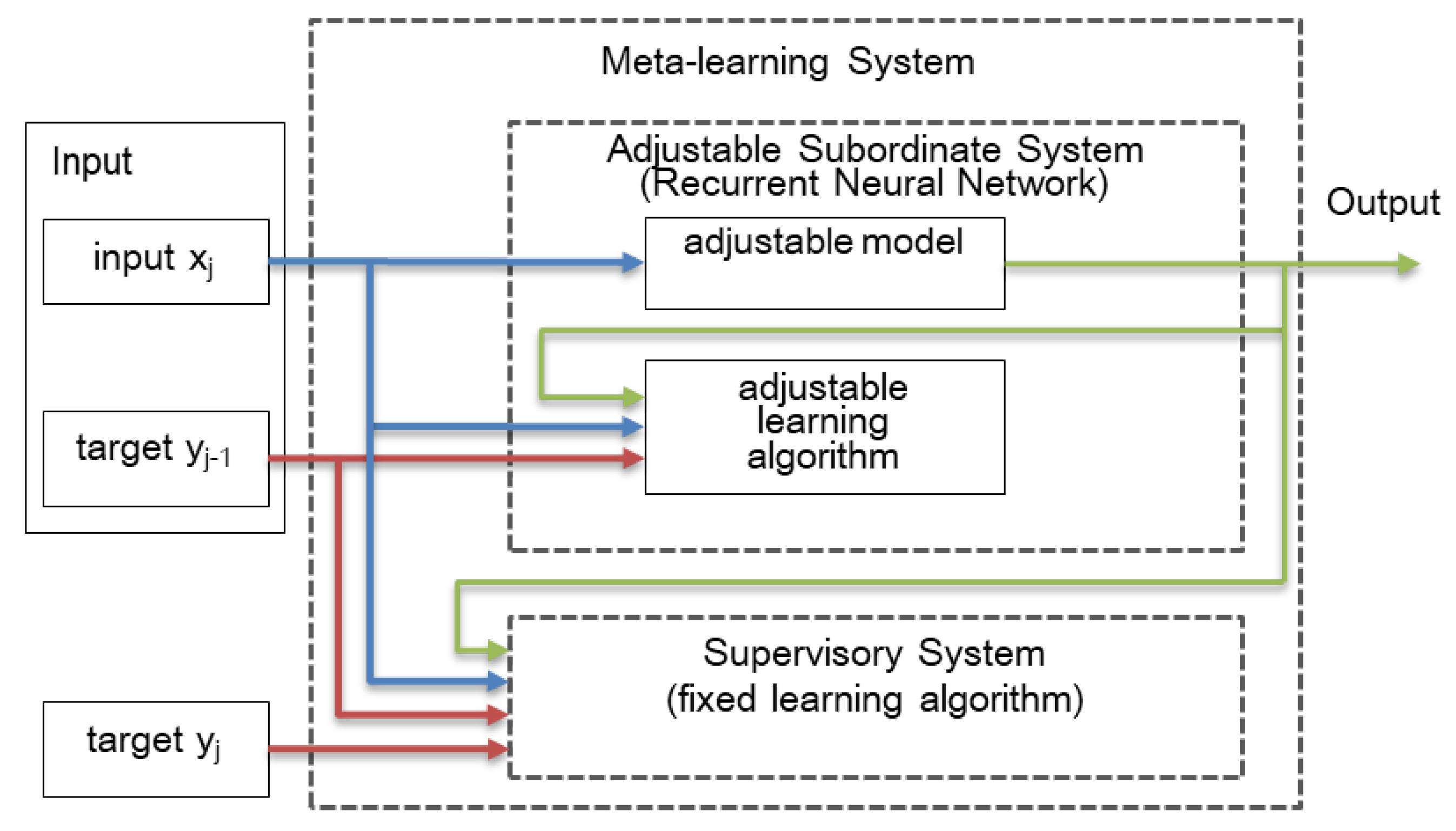
Meta-learning has been applied in many fields of machine learning/data mining. Its primary goal is to understand the interaction between a mechanism of learning and the contexts in which that mechanism is applicable. It assists machine learning systems with the process of model selection by the meta-knowledge acquired from the learning algorithms. In other words, via meta-learning, the networks could “learn how to learn” from prior experience or learned knowledge. This network learns to deal with the tasks via two stages: one acquires meta-knowledge from machine learning systems, and the other adapts that knowledge to the new problems (domain) with the objective of identifying a suitable learning algorithm or technique for them [12]. In the first stage, the learner accumulates the knowledge on the performance of multiple applications (dataset), which captures how task structure varies across the tasks. Then, whenever there is a new task to learn, the model itself fine-tunes its weighted-parameters using the small amount of the new training data to select an applicable algorithm. Meta-learning could be categorized in several ways, such as recurrent models (MANN), metric learning (Matching Network for One-shot learning), meta-optimization (Model Agnostic Meta-Learning—MAML [13]), etc. In this paper, the meta-learning system for one-shot learning tasks using recurrent architecture (Recurrent Neural Network—RNN) is applied. It follows the task set-up proposed by Hochreiter et al. [14] as pictured in Figure 1.
2.2. Meta-Learning with Memory Augmented Neural Network
In this paper, in terms of One-shot/Few-shot learning, in spite of many existing meta-learning based approaches, the Memory Augmented Neural Network proposed by A.Santoro et al. [6] is used as a model to classify unknown malware with only a few trained samples. A.Santoro et al. modify the memory access capabilities of the Neural Turing Machine (NTM) introduced by A. Graves et al. [15] to adapt this model, LRUA-MANN, to one-shot learning tasks. Although Neural Turing Machine still suffers from some problems seen in Neural Network architectures, (i.e., the fixed size of the network), it is considered a promising architecture in the future. While giving a speech in the Machine Learning Conference 2016 in San Francisco, Daniel Shank, a Senior Data Scientist at Talla, insisted that “Neural Turing Machines are a landmark architecture in the field of machine learning” [16]. Many research works and applications developed from NTM such as the Dynamic Neural Computer by A. Graves et al. [17], or the Kanerva Machine by Y. Wu et al. [18] have confirmed this. Hence, we believe that taking advantage of NTM in our approach could help it to be extended in the future.
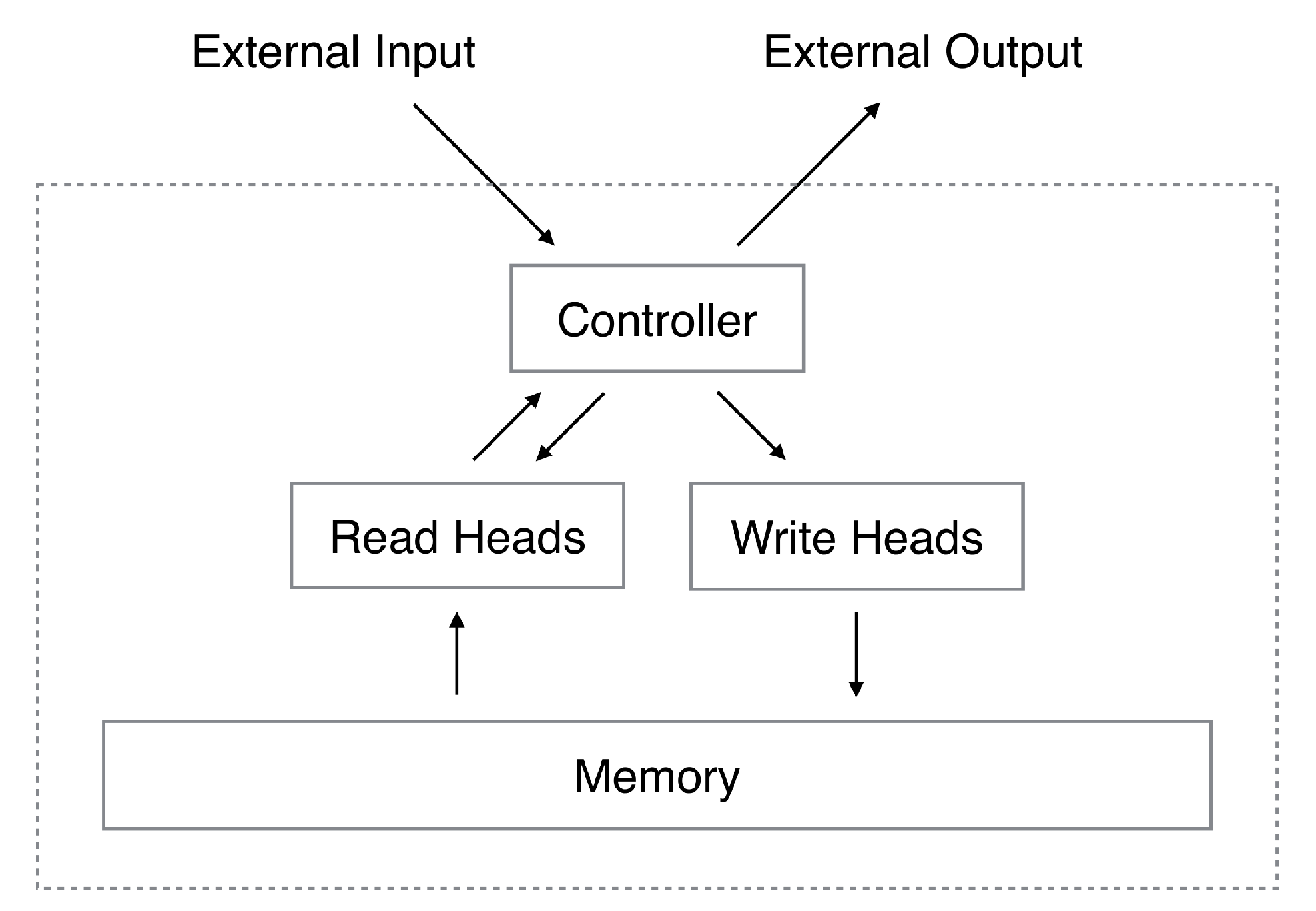
Basically, this network is fundamentally composed of four parts as NTM and is illustrated in Figure 2.
A neural network called the Controller Network receives and processes inputs, and sends its output vector to a Write Head before receiving processed data from the Read Heads, and forwards them to the output layers of the network. A simple matrix (or Memory Bank) is used to store processed data from the controllers and is considered as a memory of the whole model. The data are written into the memory from the controller via Write Head and read by the Read Heads using a special addressing mechanism called Least Recently Used Access (LRUA). In contrast to the two memory addressing mechanisms of NTM, namely content-based and location-based, LRUA allows data to be written to either the least used location (rarely-used locations) or the most recently used location (last used location) of the memory. Thanks to this mechanism, the model is advantageous to one-shot/few-shot learning sequence-based prediction tasks. More specifically, it calculates the write-weight vector as follows:
where is a sigmoid function of a scalar parameter , is the read-weight vector of a previous step, and is the least used weight vector, generated from the usage weight vector that updates every step with a decay parameter as
From this vector, an important weight called least-used weight is defined accordingly:
The notation represents the nth smallest element of . The memory will be written in accordance with this write-weight vector
The Read Heads are used to read data out of the memory. First, a Read Head computes a cosine distance between a query key vector generated from controller output and all the memory cells as
Then, this measure is used to create a read-weight vector , which is a result of its softmax function.
Finally, a read vector is generated
This read vector will be used in conjunction with the hidden state of the controller to produce an output of the network.
In general, LRUA MANN is perfect for meta-learning and one-shot/few-shot learning tasks as it could look back to the learned knowledge by both long-term memory via network’s updated weights and short-term memory of its external memories. This model overcomes the problems of the other model using RNNs, which could not perform memorization well.
Moreover, in the original paper, A.Santoro et al. did the experiments with two different neural networks as controllers, which are the Recurrent Neural Network (LSTM) and Feed Forward Network (FFN). While the LRUA-MANN with the LSTM controller could use two types of memory, e.g., Which are LSTM’s hidden cell states and Memory Bank (NTM memory cells), to save the information, the LRUA-MANN with FFN functioned as a controller use only the external memory of NTM. The LRUA-MANN using the LSTM controller seems to provide better accuracy than the one using the FFN controller since it could effectively remember the previously processed inputs.
3. Related Works
In terms of classifying malware with a few samples, there are two other relevant methods: one is Anomaly Detection, and the other is Domain Adaptation.
3.1. Anomally Detection
Anomaly detection refers to the identification of unusual objects, or outliers which are markedly different from the other known objects in the same dataset. These algorithms have broad applications in a variety of domains, such as to detect network attacks in cyber-security, to detect failures in a system and to remove anomalous data in data preprocessing step in machine learning.
In the malware analysis field, many anomaly detection algorithms have been applied [19,20,21]. Based on all valid behaviors of benign programs, anomaly detection techniques help malware detectors to detect previously unknown zero-day attacks. These methods alone themselves are not sufficient for malware detection and usually go along with other approaches to overcome their limitations, e.g., high false alarm rate and complexity [22].
To some extent, these features are related to zero-shot/one-shot/few-shot learning tasks, which are applied in this proposed approach. Both of them are used to identify never before seen malware classes based on their experience. However, the anomaly detection differs in some aspects from this proposed approach because (i) The anomaly detection techniques may identify malware that come from whether the same manifolds or not, whereas the few-shot learning model (MANN) used in this approach classifies malware based on the previously learned samples belonging to the corresponding families; and (ii) The anomaly detection normally aims to distinguish between the two contrasting objects, such as the "normal" and the "anomalous" process behaviors, the seen and the unseen malware classes. In other words, it is considered as a binary classifier, though our approach is a multi-class classifier that focuses on classifying malware into two or more classes. Although an idea of multi-class classification based anomaly detection techniques has been mentioned (e.g., Stefano et al. [23] or Barbara et al. [24]), such methodologies help classifiers to distinguish between multiple normal classes and one anomalous class; hence, they are not suitable for multi-class classification tasks as presented in this paper.
Therefore, in this paper, they are not used as comparative baselines in our approach. They ought to be significant opponents when dealing with malware-benign classification tasks.
3.2. Domain Adaptation
Another field associated with machine learning and transfer learning is Domain Adaptation. This field refers to the ability of a learning mechanism to improve performance on the target tasks after being trained in a different but related concept on a previous source task [25]. This is also the purpose of meta-learning approaches which we use in this proposed approach. In our approach, Domain adaptation is also applied as we want to adapt the trained network in the assumed known malware domain for the assumed unknown ransomware domain, makes it flexible to work well on other new malware domains in the future.
4. Proposed Method
Even though many applications of machine learning to the Malware Classification task bring very high performance (e.g., the recent works of M. Kruczkowski et al. [26], M. Ahmadi et al. [27]), such methods require hundreds of samples to be effective. In this paper, we introduce a different method that classifies malware into the proper families using only a few known samples while maintaining the acceptable level of performance. This approach could solve the “data-hungry” problem, which is a major drawback of most current machine learning algorithms.
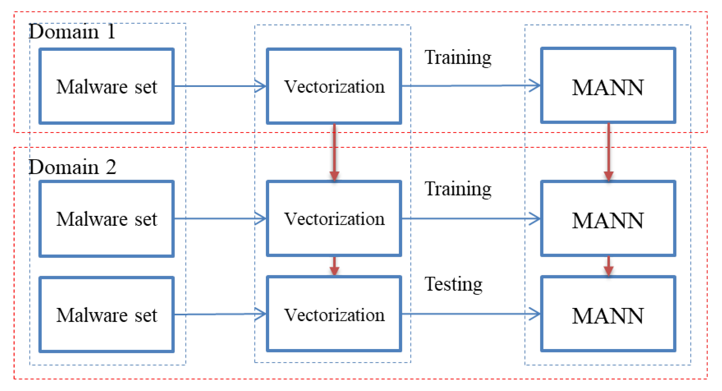
An overview of this approach is depicted in Figure 3. The proposed approach contains two different domains of learning, called Domain 1 and Domain 2. The first domain is used to train the model with already known malware types, and the other is for either training or testing with unknown types of malware dataset. The second domain is also known as the fine-tuning process in which the model is made familiar with a new dataset with a few support data.
In the second domain, the unknown malware samples are classified using the adapted model that was optimized via gradient descent during the first phase of Domain 1’s training. The model in this domain could be either trained in a few episodes with a few unknown malware samples or tested directly with the new types of malware.
Generally, the proposed method is implemented in the following five steps:
4.1. Collect Malware’s Behavior Characteristics
Depending on the malware analysis methods, e.g., static analysis and dynamic analysis, different features from malware could be collected for malware analysis. On the one hand, some useful resources of a program, such as lists of API calls (Application Programming Interface) and sequences of opcodes, are usually used in the malware static analysis. This method is often straightforward, but prone to self-encrypting (or packed), obfuscation, or self-morphing processes (e.g., polymorphic malware species). On the other hand, despite some limitations, such as time-consuming and specific environments to record malware’s behavior, the dynamic analysis could deal with the hindrances of the static analysis as it helps to analyze the behavior of malware on the fly. Since malware and benign programs use API calls, such as File IO and Registry read/write, to interact with the OS (Operating System), with the dynamic analysis methods, analysts could collect them with some process hooking libraries, e.g., Detour library [28], or EasyHook [29]. Moreover, some methods use API calls as input features to classify malware, and also bring good results; hence, API call sequences could be considered good resources to identify malware.
4.2. Extract Feature
As some kinds of malware could inject fake API calls to the regular API call sequences to cover up temporal information, and to reduce the effect of the fake API calls, we use n-gram methods to split API call sequences into different kinds of API. This idea is inspired by the work of S. Guo et al. [30] for splitting the API call sequence into some sub-sequences.
The N-gram concept is widely used in NLP (Natural Language Processing), which is simply an n-character slice of a long sentence. By sliding an n-sized window along to the sequence of API calls, the series of the n API calls are obtained. After being generated, these new n-gram APIs are converted into a numerical representation of information in the following process of vectorization.
4.3. Vectorize Feature
This step is to find the significant relationship between n-gram APIs to generate the most appropriate feature vector of each malware. A vectorization model is trained by converting all n-gram APIs of malware in Domain 1 into the specific vectors via word2vec introduced by T. Mikolov et al. [31]. The feature vector of the malware is then represented by taking an average of all converted n-gram APIs’ vectors of it.
In NLP, the word2vec model has two models, Continuous Bag-of-Words (CBOW) and Continuous Skip-grams, which are simple 2-layers neural networks, to produce word embedding. These methods are proved to be more efficient than the other NLP model in representing words. In the CBOW architecture, the model predicts the considering n-gram API by numerous surrounding APIs without regard to their order. In contrast, the continuous skip-gram architecture uses an n-gram API to predict the surrounding n-gram APIs. By working in such ways, the output vector of each API is the accumulated weights of the hidden layer. In this paper, our approach uses these models, and achieves different results according to the datasets.
4.4. Train the Memory Augmented Neural Network
We train the Neural Turing Machine using LRUA addressing mechanism to learn the meta-data of known malware samples in Domain 1. In contrast to other traditional machine learning training methods, for the meta-learning task in this training process, we guarantee that the model satisfies the rule of self-learning system, a theory of Hochreiter et al. [14]. We provide a combination of the previous output of the network and the current sample as an input to the network so that it could optimize its sub-systems itself. The input of the network is declared as a sequence of , where is a current input malware sample, is a malware class of the previous step of the sequence. Hence, the input sequence of the network is represented as the sequence .
In each training episode, the network is taught to recognize malware gradually in the sequence of samples belonged to five random malware families. This is called the 5-way classification task. These five classes are randomly grabbed from the training dataset, numbered from 0 to 4, and encoded as one-hot vector labels. These classes are different in every episode. For each class, the equal number of malware samples of the corresponding class is randomly sampled.
The output at time step t of the Memory Augmented Neural Network is defined according to the definition in Section 2.2. In general, it could be rewritten as the function of the whole MANN network:
where is a combination of the vectorized malware sample and the class of the previous malware sample in a sequence at time t. and are the previous states of the MANN’s controller (LSTM). is a specific value read from the memory of the previous step.
Then, the classification result is a categorical distribution of the output using weights from MANN’s output to the linear output layer
This network is trained for thousands of episodes so that the output of the classification task could reach an acceptable threshold. Then, this optimized model is transferred to Domain 2 to test with unknown data.
4.5. Adapt Trained Network to the New Domain
In this step, we adapt the trained network in the previous step to classify the new kinds of malware. The trained word2vec model in Domain 1 is used to generate feature vectors of the new samples. It is noticed that the new malware samples might not contain n-gram APIs collected and vectorized by trained word2vec model in Domain 1. In such cases, they are eliminated in a calculation of the new feature vector. The number of non-existence n-gram APIs could be reduced if we collect enough malware samples in Domain 1.
For some tasks, if there are enough samples of new malware types, we could use some of them to fine-tune the model before doing classification tasks with the unknown samples to increase final accuracies. Otherwise, these unknown malware could be directly classified with the pre-trained model.
The training and testing procedures in this domain are the same as in Domain 1.
5. Experiments
In this paper, the experiments with two models on two different datasets are described. One model uses LSTM as a controller as the original paper, and the other uses the Gated Recurrent Unit (GRU) as a controller. LSTM and GRU are two closely related recurrent units of the recurrent neural network (RNN), which is an extension of a conventional Feed Forward Neural Network. While LSTM introduced by Hochreiter and Schmidhuber has had a long history of application since 1997, GRU was first implemented in 2014 by Cho at al. [32]. It is slightly less complex but approximately as good as an LSTM performance-wise. The key difference between them is that GRU has two gates (reset and update gates), while LSTM has three gates (namely input, output, and forget gates). According to empirical evaluations of these RNN units [33,34], GRU could outperform LSTM in terms of convergence in CPU time, the number of parameters, as well as the performance in some cases. In our experiments, they provide different performance according to the datasets.
5.1. Hyper Parameters
For the vectorization process, we use the word2vec model and vary its parameters to generate different feature vectors. Specifically, we try our model with different input features according to the following factors of the word2vec model:
- N-gram: The number of API calls are used to create a new n-gram API.
- Min-count: A threshold such that all n-gram APIs with total frequency in a malware’s API sequence lower than it will be ignored.
- Window-size: Maximum distance between the current and predicted word within a sentence.
- Vector-size: Dimensionality of the malware vectors.
- Word2vec model: A selection between two models of word2vec model, skip-gram or CBOW model.
In addition, we set the parameters of the MANN network in all experiments as follows: (1) ADAM optimizer with a learning rate of 0.95; (2) LRUA-MANN network uses the external memory with 128 memory slots of size 40, 200 hidden units for LSTM controller (or GRU controller), 4 read heads, 1 write head, usage decay of write weights of 0.99, mini-batch size of 16. With these hyper-parameters, we achieved the best results.
5.2. Case 1: FFRI 2017 Dataset
The FFRI dataset is a part of the anti-Malware engineering WorkShop (MWS) dataset, which is designed for use in anti-malware research. The data has been collected and created every year since 2013 using the dynamic malware analysis system Cuckoo Sandbox and Yarai Analyzer Professional by a private company FFRI. In this paper, we use the FFRI 2017 dataset collected from March 2017 to April 2017 [10]. This dataset is a log of total 6251 malware samples, in which most of them were selected randomly from a massive collection of malware by crawling the web sites, online malware services reflecting the trends of the malware at that time such as Virustotal, solely in Portable Executable (PE) format. Each malware’s activities are recorded via Cuckoo sandbox in 90 s and are provided in a JSON format.
In this experiment, we assume that we have already known many types of malware except ransomware, and the task is to classify ransomware into the assigned classes with very little knowledge of them. For that purpose, the dataset is divided into two subsets, one contains only the ransomware types, and the other is the rest of the FFRI 2017 dataset. By splitting the dataset in this way, we could verify the ability of the model that deals with never seen before ransomware samples. All classes on this dataset that have more than ten samples are collected. On the known malware dataset, there are 45 classes with a total of 4154 malware samples. The ransomware dataset contains nine ransomware classes with 1574 ransomware samples. These classes are listed in Table 1.
We train our model in Domain 1, which consists of the known types of malware, and use this trained model to classify ransomware in Domain 2.
5.2.1. Training of the Model in Domain 1
Firstly, we split the API Sequences of every record (malware) in the first dataset into n-grams. According to the results achieved from experiments, if we use 1-gram to split API sequences, we could get the best results. Secondly, we train the word2vec network with those new samples with a variety of hyper- parameters such as window-size, model types (i.e., skip-gram and CBOW), etc. Then, the malware’s feature vector is calculated as the average value of all converted n-gram sliced API vectors of the corresponding malware. Next, we train the model to do 5-way classification tasks (classify malware into five categories). In this task, for each episode, ten samples of each malware class are randomly chosen to create an input sequence of fifty samples (five malware families with ten samples each) and fed to the LRUA-MANN. The model is trained to classify samples in this sequence one by one into five different categories numbered from 0 to 4 (these categories are different from the malware families). Particularly, after randomly guessing the first sample of the sequence on the 5-way classification task, the model will classify the next instance based on its knowledge of the previous samples stored in the memory and so forth.
The training process is terminated after 200,000 episodes. To calculate the loss of the training, we use categorical cross-entropy as a loss function for multi-class classification. This loss value gradually reduces after some thousands of episodes of training, and the trained model with the lowest loss value is selected for the unknown ransomware classification tasks in Domain 2.
5.2.2. Classification of the Unknown Ransomware in Domain 2
The trained models with the lowest loss value in Domain 1 are selected to guarantee the best accuracy in the unknown ransomware dataset. The two experiments are implemented in this domain: (i) use the pre-trained model without any modification in Domain 2 to predict the unknown ransomware, and (ii) fine-tune the pre-trained models with 11 samples of each ransomware family, and then test them with the rest of the ransomware dataset in Domain 2.
In the first experiments, they are conducted with many parameter-dependent models. Among them, the best results of 71.99% accuracy after examining 9 samples are obtained when we use the skip-gram model with the window-size parameter of 50 and the min-count parameter of 2 to convert 1-gram APIs into a vector of 50 dimensions. Table 2 demonstrates the results of the model using LSTM as a controller with five different word2vec parameter settings.
We also compare the performance of the model when using different controllers. According to Table 3, the MANN model using LSTM outperforms the one using GRU from the second instance’s accuracy.
Regarding the baselines, to the best of our knowledge, it seems that there are no other one-shot/few-shot learning methods for classifying malware using API call sequences so far. Therefore, to verify our result, we use some traditional classifiers such as Support Vector Machine (SVM), Random Forest, Feed-Forward Network, and Nearest Neighbors. We also use other RNNs (i.e., LSTM and GRU) to classify ransomware families as the baselines under the same test condition as our approach.
According to Table 1, we found the unbalanced categories in the ransomware dataset. for example, the family trojan-ransom.win32.shade has only 21 samples while trojan-ransom.win32.blocker family has 555 samples. Although this imbalance does not influence our model as we pick randomly five samples each class each time, it could impact the final result of the baselines. It can be reduced to a great extent by under-sampling the majority classes and making them close to that of trojan-ransom.win32.shade class. Hence, we randomly select 21 samples from each class to create a subset of 105 samples for each experiment.
Except for the experiments conducted with RNN, which is the same with the MANN model, we run the experiments of the baselines (traditional machine learning methods) with five and nine random samples from each class for training and the rest for testing. These experiments correspond to the 6th and 10th instance of the MANN model’s experiments, respectively. In both experiments, the baselines are reset to train and test 1000 times, and the final accuracies of these baselines are the averages of their accuracies. These results are then compared with the results of the 6th instance and 10th instance of the MANN model, respectively. In both cases, the proposed models overcome all six baseline models. Regarding the baselines’ results, except for the K-NN model with very low accuracies (25.63% and 32.76% for the 6th instance and the 10th instance, respectively), other baselines could reach up to around 50% in these experiments. However, these results are not higher than ours in both cases. The results show that the MANN model using LSTM as the controller is better than using GRU in these experiments (69.58% and 71.99% with LSTM as controller compared to 66.38% and 68.44% of the MANN model with GRU as controller). The detailed results are listed in Table 4.
If we spend a few data in Domain 2 for fine-tuning the pre-trained models, we could improve their overall performance. Table 5 shows the results of the 5-class classification tasks after the fine-tuning process. In these experiments, both baseline models and MANN are pre-trained with a total of 55 samples, in which 11 samples of each class are randomly selected. The test results of the pre-trained baselines without any training correspond to the first instance in the experiments of the MANN model. In other cases, we train the baselines with either one, five or nine random samples of each feeding class. The results are compared with the proposed approaches at the 2nd, 6th and 10th instances accordingly. Note that, even when fine-tuning, this setup still follows the same procedure as the previous experiments as the assigned class is a random number. The results are very competitive since the MANN model using GRU as a controller could guess correctly 84.59% at the 2nd, 90.8% at the 6th and 91.77% at the 10th instance, overcoming the other baselines such as LSTM with 81.63%, 90.88% and 87.08%, or SVM with 83.32%, 83.51%, and 84.22%, respectively.
5.3. Case 2: API-Based Malware Detection System Dataset
In this experiment, we use a dataset collected and shared by Huy Kang Kim et al. [11]. This API-based Malware Detection System (APIMDS) dataset contains with 23,080 malware samples picked randomly from the Malicia project [35] and VirusTotal [36]. It was shared online via Hacking and Countermeasure Research Lab in the Graduate School of Information Security of the Korea University. This dataset is summarized in Table 6.
The same experiments as the FFRI 2017 dataset in the previous section are conducted. We split this dataset into two smaller subsets. One contains all assumed known malware, which is all types of malware in this dataset except the ransomware types, and the other has only ransomware samples. Table 7 lists all ransomware classes and their number of samples.
There is also an imbalance in the ransomware dataset like in the FFRI 2017 dataset. For example, the Trojan-ransom.win32.blocker family has only 18 samples while the others have more than 84 samples. For the baselines, we try to balance the number of samples in all classes by reducing the number of other classes to the number of samples of the Trojan-ransom.win32.blocker family. These samples are randomly changed according to the experiments with the traditional classifiers.
In the first domain, the malware samples on the APIMDS dataset are converted into feature vectors via the word2vec model using various settings of the parameters. The final results of the model in Domain 2 shows that if the 250-sized feature vectors are generated using the CBOW model with 5-sized window-size, 1-gram, and min-count of 1, the models could produce the best accuracy. A comparison of this setting with the others is detailed in Table 8. Compared to the setting that works best on the FFRI 2017 dataset, in this dataset, 250-sized feature vectors generated by the CBOW model give us the best performance.
The models using different controllers are also examined on this dataset. According to Table 9, the MANN model using GRU controller outperforms the one using LSTM only in the first few instances.
Our models also show superior results over the baselines. Apart from the KNN classifier with a very low rate of 28.65%, the other traditional methods could categorize ransomware samples into the correct classes with just around 50% accurate. These results are indicated in Table 10.
In the case of fine-tuning, again, our pre-trained models and the baselines are fed 40 samples for fine-tuning, in which eight samples are randomly taken from each class, leaving the rest ten samples in each class for testing. Generally, it improves all the performance of our models and the baselines. As indicated in Table 11, although the classification rates of the first instance of the MANN models are lower than the baselines (i.e., 43.02% with GRU controller, and over 71% of the baselines), the second instance could be classified with a higher rate as above 75% with the model using the LSTM controller and 80.55% with the one using the GRU controller. From the 6th samples, the model using LSTM could classify correctly over 89% while SVM, Nearest Neighbors (with K = 4), MLP, and RF are almost the same with 78.09%, 56.02%, 78.58%, and 70.98% respectively. The RNN models could not overcome the MANN models, although they were better than the machine learning methods.
5.4. Discussion
In this section, we have evaluated the proposed approach on the two datasets. The results provided by the experiments are also different according to many factors.
Firstly, the best results achieved with the Skip-gram model on the FFRI 2017 dataset, and with the CBOW model on the APIMDS dataset have shown that the most important influence on this approach is how to select the best-fit word embedding model regarding the dataset. Both the Skip-gram model and the CBOW model with various settings show their advantages and disadvantages. According to Mikolov et al. [31], Skip-gram model works well with a small amount of the training data, whereas CBOW is several times faster than train, slightly better accuracy for the frequent APIs. They are correct in our cases. While only 4154 samples on the FFRI 2017 dataset were used to train the model, nearly 22,650 samples extracted from the APIMDS dataset were used. Hence, depending on the size of the dataset, we could specify the best word embedding model for our approach.
Secondly, we also consider the MANN model’s parameters as another vital factor. Since the MANN model is one of the two important components of this approach, its network parameters, such as controller types and memory size, decide the suitable model in accordance with the specific dataset and the number of used samples. For example, in our experiments, the model equipped with LSTM seems to adapt better with a few samples, but it is better to use GRU as the controller in some other cases when there are more data to learn. However, it is necessary to conduct more experiments with different datasets before deciding the best controller for this approach.
Thirdly, the way of recording API calls of malware is another factor that influences the final performance. While the APIMDS dataset provides the API calls of each malware as a sorted sequence following the sampling methods of the authors, the FFRI 2017 dataset stores API calls of the malware separately according to their recording times in JSON format. Consequently, it might make the difference in the structure of the API call sequences between the two datasets.
Finally, how to merge API calls into a new one using n-gram also contributes to the final results of the model. On these datasets, unigram is the best value among n-grams that improves the quality of the models’ inputs. As mentioned in the previous sections, it seems that unigram is useful to not only extract important features but also eliminate the effect of the faked injected APIs in malware samples.
Therefore, to conclude, depending on the malware data, many aspects need to be considered to increase the efficiency of this approach.
6. Conclusions
The early detection and prevention of dangers from threats such as spreading of malware, zero-day exploits, etc. in defense systems of small networks, organization network as well as the whole internet, is an essential area of cyber-security research. Almost all of the recently proposed malware classification methods require tons of malware samples to achieve accepted accuracies. To overcome this problem, the proposed approach takes advantage of the AI developments to introduce a novel way that could help malware analysts quickly classify malware into the correct groups, even with only a few known samples.
In this paper, the effectiveness of malware classification based on Natural Language Processing in combination with Memory Augmented Neural Network for the one-shot learning task has been shown. The accuracies of the proposed approach are quite good, even if only one sample is recognized. Furthermore, these results could be improved by adjusting the hyper-parameters of the Neural Turing Machine and parameters of the word2vec model; however, this makes the approach parameter-independent. Therefore, it is necessary to continue to undertake deeper research into this disadvantage before applying it to practice.
As future work, on the one hand, we will take a deeper look at some other one-shot learning algorithms to find more suitable methods for malware analysis to improve the accuracy of our approach. Also, the evaluation methods will be considered and conducted more precisely so that the proposed approaches could be accurately evaluated. On the other hand, we will also try to collect more benign programs as well as different kinds of malware’s API sequences. Hence, we could re-evaluate our methods to detect and distinguish malware from the benign-ware well.
Finally, because this is only the beginning of research that applies one-shot learning algorithms in the machine learning field to malware analysis and cyber-security, we hope our contribution could create a paradigm for future studies of the malware research, and provide malware analysts a new way to classify malware even with a few samples.
Author Contributions
K.T. developed the theory, performed the computations and carried out the experiment under supervise of H.S. and M.K.; K.T. and H.S. wrote the manuscript with support from M.K.; H.S. and M.K. helped supervise the findings of this work. All authors have read and agreed to the published version of the manuscript.
Funding
This research received no external funding.
Conflicts of Interest
The authors declare no conflicts of interest.
References
- Kaspersky. Kaspersky Lab Report. Available online: https://www.kaspersky.com/about/press-release/2017kaspersky-lab-detects-360000-new-malicious-files-daily (accessed on 10 November 2019).
- Symantec Corporation. ISTR-Internet Security Threat Report. February 2019; Volume 24. Available online: https://www.symantec.com/content/dam/symantec/docs/reports/istr-24-2019-en.pdf (accessed on 18 August 2019).
- Li, F.-F.; Fergus, R.; Perona, P. One-shot learning of object categories. IEEE Trans. Partern Anal. Mach. Intell. 2006, 28, 594–611. [Google Scholar]
- Lake, B.M.; Salakhutdinov, R.; Tenenbaum, J.B. Human-level concept learning through probabilistic program induction. Science 2015, 350, 1332–1338. [Google Scholar] [CrossRef] [PubMed] [Green Version]
- Salakhutdinov, R.; Tenenbaum, J.B.; Torralba, A. One-shot learning with a hierarchical nonparametric bayesian model. J. Mach. Learn. Res. Proc. Track. 2012, 27, 195–207. [Google Scholar]
- Santoro, A.; Bartunov, S.; Botvinick, M.; Wierstra, D.; Lillicrap, T. Meta-learning with memory-augmented neural networks. In Proceedings of the 33rd International Conference on International Conference on Machine Learning, New York, NY, USA, 19–24 June 2016; Volume 48, pp. 1842–1850. [Google Scholar]
- Vinyals, O.; Blundell, C.; Lillicrap, T.; Kavukcuoglu, K.; Wierstra, D. Matching networks for one shot learning. arXiv 2016, arXiv:1606.04080, 3630–3638. [Google Scholar]
- Koch, G.; Zemel, R.; Salakhutdinov, R. Siamese neural networks for one-shot image recognition. Deep Learning Workshop (ICML), Lille Metropole, France, 10–11 July 2015. Available online: https://sites.google.com/site/deeplearning2015/accepted-papers (accessed on 6 January 2020).
- Tran, T.K.; Sato, H.; Kubo, M. One-shot Learning Approach for Unknown Malware Classification. In Proceedings of the 2018 5th Asian Conference on Defense Technology (ACDT), Hanoi, Vietnam, 25–27 October 2018; pp. 8–13. [Google Scholar] [CrossRef]
- FFRI Company. Introduction to FFRI 2017 Dataset. Available online: https://www.iwsec.org/mws/2017/20170606/FFRI_Dataset_2017.pdf (accessed on 18 August 2018). (In Japanese).
- Kim, H.K. API-Based Malware Detection System Dataset. Available online: http://ocslab.hksecurity.net/apimds-dataset (accessed on 18 August 2017).
- Brazdil, P.; Vilalta, R.; Giraud-Carrier, C.; Soares, C. Metalearning. In Encyclopedia of Machine Learning and Data Mining; Sammut, C., Webb, G.I., Eds.; Springer: New York, NY, USA, 2017; pp. 818–823. [Google Scholar]
- Finn, C.; Abbeel, P.; Levine, S. Model-agnostic meta-learning for fast adaptation of deep networks. In Proceedings of the 34th International Conference on Machine Learning, Sydney, Australia, 6–11 August 2017; Volume 70, pp. 1126–1135. [Google Scholar]
- Hochreiter, S.; Younger, A.S.; Conwell, P.R. Learning to learn using gradient descent. In Proceedings of the International Conference on Artificial Neural Networks (ICANN 2001), Vienna, Austria, 21–25 August 2001; pp. 87–94. [Google Scholar]
- Graves, A.; Wayne, G.; Danihelka, I. Neural turing machines. arXiv 2014, arXiv:1410.5401. [Google Scholar]
- Daniel, S. Neural Turing Machines: Perils and Promise. Machine Learning Conference 2016. Available online: https://mlconf.com/sessions/neural-turing-machines-are-a-landmark-architecture/ (accessed on 8 December 2019).
- Graves, A.; Wayne, G.; Reynolds, M.; Harley, T.; Danihelka, I.; Grabska-Barwińska, A.; Colmenarejo, S.G.; Grefenstette, E.; Ramalho, T.; Agapiou, J.; et al. Hybrid computing using a neural network with dynamic external memory. Nature 2016, 538, 471–476. [Google Scholar] [CrossRef] [PubMed]
- Wu, Y.; Wayne, G.; Graves, A.; Lillicrap, T. The Kanerva Machine: A Generative Distributed Memory. arXiv 2018, arXiv:1804.01756. [Google Scholar]
- Teng, H.S.; Chen, K.; Lu, S.C. Adaptive real-time anomaly detection using inductively generated sequential patterns. In Proceedings of the 1990 IEEE Computer Society Symposium on Research in Security and Privacy, Oakland, CA, USA, 7–9 May 1990; pp. 278–284. [Google Scholar]
- Garcia-Teodoro, P.; Diaz-Verdejo, J.; Macia-Fernandez, G.; Vazquez, E. Anomaly-based network intrusion detection:Techniques, systems and challenges. Comput. Secur. 2009, 28, 18–28. [Google Scholar] [CrossRef]
- Burnaev, E.; Smolyakov, D. One-Class SVM with Privileged Information and Its Application to Malware Detection. In Proceedings of the 2016 IEEE 16th International Conference on Data Mining Workshops (ICDMW), Barcelona, Spain, 12–15 December 2016; pp. 273–280. [Google Scholar] [CrossRef] [Green Version]
- Idika, N.C.; Mathur, A.P. A Survey of Malware Detection Techniques. 2007. Available online: http://citeseerx.ist.psu.edu/viewdoc/download?doi=10.1.1.75.4594&rep=rep1&type=pdf (accessed on 6 January 2020).
- Stefano, C.; Sansone, C.; Vento, M. To reject or not to reject: that is the question–an answer in case of neural classifiers. IEEE Trans. Syst. Manag. Cybern. 2000, 30, 84–94. [Google Scholar] [CrossRef]
- Barbara, D.; Couto, J.; Jajodia, S.; Wu, N. Detecting novel network intrusions using bayes estimators. In Proceedings of the First SIAM International Conference on Data Mining, Chicago, IL, USA, 5–7 April 2001; pp. 1–17. [Google Scholar]
- Vilalta, R.; Giraud-Carrier, C.; Brazdil, P.; Soares, C. Inductive Transfer. In Encyclopedia of Machine Learning and Data Mining; Sammut, C., Webb, G.I., Eds.; Springer: New York, NY, USA, 2017; pp. 666–671. [Google Scholar]
- Kruczkowski, M.; Szynkiewicz, E.N. Support vector machine for malware analysis and classification, Web Intelligence (WI) and Intelligent Agent Technologies (IAT). IEEE Comput. Soc. 2014, 2, 415–420. [Google Scholar]
- Ahmadi, M.; Giacinto, G.; Ulyanov, D.; Semenov, S.; Trofimov, M. Novel feature extraction, selection and fusion for effective malware family classification. In Proceedings of the Sixth ACM Conference on Data and Application Security and Privacy (CODASPY), New Orleans, LA, USA, 9–11 March 2016; pp. 183–194. [Google Scholar]
- MicroSoft Github Source Code. Available online: https://github.com/microsoft/Detours (accessed on 8 December 2019).
- Christoph Husse, H.; Justin, S. Easy Hook Source Code. Available online: https://easyhook.github.io/ (accessed on 8 December 2019).
- Guo, S.; Yuan, Q.; Lin, F.; Wang, F.; Ban, T. A malware detection algorithm based on multi-view fusion. In Proceedings of the 17th International Conference on Neural Information Processing: Models and Applications, Sydney, Australia, 22–25 November 2010; pp. 259–266. [Google Scholar]
- Mikolov, T.; Chen, K.; Corrado, G.; Dean, J. Efficient estimation of word representations in vector space. arXiv 2013, arXiv:1301.3781. [Google Scholar]
- Cho, K.; van Merrienboer, B.; Gulcehre, C.; Bougares, F.; Schwenk, H.; Bengio, Y. Learning phrase representations using RNN encoder decoder for statistical machine translation. In Proceedings of the 2014 Conference on Empirical Methods in Natural Language Processing (EMNLP), Doha, Qatar, 25–29 October 2014; pp. 1724–1734. [Google Scholar]
- Chung, J.; Caglar, G.; Cho, K.; Bengio, Y. Empirical evaluation of gated recurrent neural networks on sequence modeling. arXiv 2014, arXiv:1412.3555. [Google Scholar]
- Rafal, J.; Wojciech, Z.; Ilya, S. An empirical exploration of recurrent network architectures. In Proceedings of the 32nd International Conference on Machine Learning (ICML-15), Lille, France, 6–11 July 2015; pp. 2342–2350. [Google Scholar]
- Malicia, P. Available online: http://malicia-project.com/dataset.html (accessed on 6 January 2020).
- Virus Total. Available online: https://virustotal.com (accessed on 6 January 2020).
- Ki, Y.; Kim, E.; Kang, K.H. A novel approach to detect malware based on API call sequence analysis. Int. J. Distrib. Sens. Netw. 2015, 11, 659101. Available online: https://0-journals-sagepub-com.brum.beds.ac.uk/doi/full/10.1155/2015/659101 (accessed on 6 January 2020). [CrossRef] [Green Version]
Figure 1.
Overview of the Meta-learning system using Recurrent Neural Network. The subordinate system plays a role as a self-adjustable system.
Figure 1.
Overview of the Meta-learning system using Recurrent Neural Network. The subordinate system plays a role as a self-adjustable system.

Figure 2.
An architect of Neural Turing Machine consists of 4 parts: a controller, a write head, read heads and Memory (excerpt from [15]).
Figure 2.
An architect of Neural Turing Machine consists of 4 parts: a controller, a write head, read heads and Memory (excerpt from [15]).

Figure 3.
The proposed method contains two domains: the model is trained with familiar malware families in the first domain while in the second domain, the pre-trained model is used to classify unknown malware types with very few samples.
Figure 3.
The proposed method contains two domains: the model is trained with familiar malware families in the first domain while in the second domain, the pre-trained model is used to classify unknown malware types with very few samples.


Table 1.
Ransomware families of the FFRI 2017 dataset.
| Families | Number of Samples |
|---|---|
| trojan-ransom.win32.shade | 21 |
| trojan-ransom.win32.foreign | 23 |
| trojan-ransom.win32.crusis | 27 |
| trojan-ransom.win32.locky | 41 |
| trojan-ransom.win32.spora | 50 |
| trojan-ransom.win32.sagecrypt | 60 |
| trojan-ransom.win32.genericcryptor | 95 |
| trojan-ransom.win32.blocker | 555 |
| trojan-ransom.win32.zerber | 702 |
Table 2.
Accuracies of the first ten instances without training in Domain 2 of the model using LSTM as a controller. The best result is archived by using feature vectors generated from word2vec in the skip-gram model with the following parameters: n-gram of 1, vector-size of 50, window-size of 5, min-count of 2.
| Model | Vector Size | Window Size | Min-Count | n-Gram | 6th | 10th |
|---|---|---|---|---|---|---|
| Skip-gram | 50 | 5 | 2 | 1 | 69.58 | 71.99 |
| Skip-gram | 200 | 4 | 1 | 1 | 64.5 | 67.05 |
| CBOW | 50 | 5 | 2 | 2 | 58.18 | 61.35 |
| CBOW | 100 | 5 | 1 | 1 | 55.94 | 58.91 |
| CBOW | 250 | 5 | 1 | 1 | 55.37 | 58.63 |
Table 3.
A comparison of the model using two types of controller: LSTM and Gated Recurrent Unit (GRU).
Table 3.
A comparison of the model using two types of controller: LSTM and Gated Recurrent Unit (GRU).
| Controller | 1st | 2nd | 3rd | 4th | 6th | 10th |
|---|---|---|---|---|---|---|
| LSTM | 20.03 | 53.86 | 64.41 | 65.75 | 69.58 | 71.99 |
| GRU | 28.5 | 51.62 | 58.4 | 62.36 | 66.38 | 68.44 |
Table 4.
Accuracies of the first ten instances without training in Domain 2 of the FFRI 2017 dataset. The best result is archived by using feature vectors generated from word2vec in the skip-gram model with the parameters: n-gram of 1, vector-size of 50, window-size of 5, min-count of 2.
Table 4.
Accuracies of the first ten instances without training in Domain 2 of the FFRI 2017 dataset. The best result is archived by using feature vectors generated from word2vec in the skip-gram model with the parameters: n-gram of 1, vector-size of 50, window-size of 5, min-count of 2.
| Model | Controller | 6th | 10th |
|---|---|---|---|
| MANN | LSTM | 69.58 | 71.99 |
| MANN | GRU | 66.38 | 68.44 |
| LSTM | - | 52.17 | 52.86 |
| GRU | - | 51.78 | 53.27 |
| SVM | - | 52.56 | 60.51 |
| KNN (K = 4) | - | 25.63 | 32.76 |
| MLP | - | 52.49 | 60.97 |
| RF | - | 45.06 | 51.82 |
Table 5.
In the case of fine-tuning, the previous model is continued to train with 11 samples each class of ransomware before classifying the remains ransomware samples in Domain 2 dataset.
Table 5.
In the case of fine-tuning, the previous model is continued to train with 11 samples each class of ransomware before classifying the remains ransomware samples in Domain 2 dataset.
| Model | Controller | 1st | 2nd | 6th | 10th |
|---|---|---|---|---|---|
| MANN | LSTM | 41.16 | 83.36 | 89.78 | 90.59 |
| MANN | GRU | 40.53 | 84.59 | 90.88 | 91.77 |
| LSTM | - | 40.28 | 81.63 | 86.58 | 87.08 |
| GRU | - | 39.99 | 81.01 | 86.10 | 86.63 |
| SVM | - | 82.88 | 83.32 | 83.51 | 84.22 |
| KNN (K = 4) | - | 80.02 | 80.69 | 80.51 | 81.53 |
| MLP | - | 85.10 | 84.93 | 84.98 | 85.21 |
| RF | - | 80.40 | 81.96 | 81.56 | 82.52 |
Table 6.
API-based malware detection system dataset description. Excerpt from [37].
Table 6.
API-based malware detection system dataset description. Excerpt from [37].
| Category | Subcategory | Ratio (%) |
|---|---|---|
| Backdoor | - | 3.37 |
| Worm | Worm | 3.32 |
| Email-Worm | 0.55 | |
| Net-Worm | 0.79 | |
| P2P-Worm | 0.3 | |
| Packed | - | 5.57 |
| PUP | Adware | 13.63 |
| Downloader | 2.94 | |
| WebToolbar | 1.22 | |
| Trojan | Trojan (Generic) | 29.3 |
| Trojan-Banker | 0.14 | |
| Trojan-Clicker | 0.12 | |
| Trojan-Downloader | 2.29 | |
| Trojan-Dropper | 1.91 | |
| Trojan-FakeAV | 18.8 | |
| Trojan-GameThief | 0.63 | |
| Trojan-PSW | 3.79 | |
| Trojan-Ransomware | 2.58 | |
| Trojan-Spy | 3.12 | |
| Misc. | - | 5.52 |
Table 7.
Ransomware families of Domain 2 dataset.
| Families | Samples |
|---|---|
| trojan-ransom.win32.blocker | 18 |
| trojan-ransom.win32.mbro | 84 |
| trojan-ransom.win32.agent | 93 |
| trojan-ransom.win32.pornoasset | 90 |
| trojan-ransom.win32.foreign | 145 |
Table 8.
Accuracies of the first ten instances without training in Domain 2 of the model using LSTM as a controller. On the APIMDS dataset, the best model is achieved by using feature vectors generated from the word2vec in the CBOW model with the parameters: n-gram of 1, vector-size of 250, window-size of 5, min-count of 1.
| Model | Vector Size | Window Size | Min-Count | n-Gram | 6th | 10th |
|---|---|---|---|---|---|---|
| CBOW | 250 | 5 | 1 | 1 | 75.66 | 78.85 |
| Skip-gram | 50 | 5 | 2 | 1 | 64.86 | 69.66 |
| Skip-gram | 200 | 4 | 1 | 1 | 68.0 | 7268 |
| CBOW | 50 | 5 | 2 | 2 | 55.51 | 60.61 |
| CBOW | 100 | 5 | 1 | 1 | 73.44 | 77.47 |
Table 9.
A comparison of the model using 2 types of controller: LSTM and GRU.
| Controller | 1st | 2nd | 3rd | 4th | 6th | 10th |
|---|---|---|---|---|---|---|
| LSTM | 16.61 | 53.20 | 64.77 | 70.24 | 75.66 | 78.85 |
| GRU | 13.70 | 54.51 | 66.55 | 71.74 | 75.53 | 77.21 |
Table 10.
Accuracies of the first ten instances without training in Domain 2.
| Model | Controller | 6th | 10th |
|---|---|---|---|
| MANN | LSTM | 75.66 | 78.85 |
| MANN | GRU | 75.53 | 77.21 |
| LSTM | - | 59.90 | 62.54 |
| GRU | - | 65.41 | 68.65 |
| SVM | - | 41.26 | 51.58 |
| KNN (K = 4) | - | 19.57 | 28.65 |
| MLP | - | 49.2 | 52.81 |
| RF | - | 39.79 | 45.91 |
Table 11.
In the case of fine-tuning, the previous model is continued to train with eight samples each class of ransomware before classifying the remains ransomware samples in Domain 2 dataset.
Table 11.
In the case of fine-tuning, the previous model is continued to train with eight samples each class of ransomware before classifying the remains ransomware samples in Domain 2 dataset.
| Model | Controller | 1st | 2nd | 6th | 10th |
|---|---|---|---|---|---|
| MANN | LSTM | 32.46 | 75.92 | 88.98 | 89.59 |
| MANN | GRU | 34.02 | 80.55 | 88.3 | 88.73 |
| LSTM | - | 33.38 | 77.19 | 80.45 | 80.62 |
| GRU | - | 33.68 | 80.19 | 83.29 | 83.64 |
| SVM | - | 78.3 | 78.5 | 78.09 | 79.56 |
| KNN (K = 4) | - | 54.4 | 55.0 | 56.02 | 57.41 |
| MLP | - | 78.24 | 78.87 | 78.58 | 78.85 |
| RF | - | 71.72 | 70.39 | 70.98 | 73.27 |
© 2020 by the authors. Licensee MDPI, Basel, Switzerland. This article is an open access article distributed under the terms and conditions of the Creative Commons Attribution (CC BY) license (http://creativecommons.org/licenses/by/4.0/).
Share and Cite
MDPI and ACS Style
Tran, K.; Sato, H.; Kubo, M. MANNWARE: A Malware Classification Approach with a Few Samples Using a Memory Augmented Neural Network. Information 2020, 11, 51. https://0-doi-org.brum.beds.ac.uk/10.3390/info11010051
AMA Style
Tran K, Sato H, Kubo M. MANNWARE: A Malware Classification Approach with a Few Samples Using a Memory Augmented Neural Network. Information. 2020; 11(1):51. https://0-doi-org.brum.beds.ac.uk/10.3390/info11010051
Chicago/Turabian StyleTran, Kien, Hiroshi Sato, and Masao Kubo. 2020. "MANNWARE: A Malware Classification Approach with a Few Samples Using a Memory Augmented Neural Network" Information 11, no. 1: 51. https://0-doi-org.brum.beds.ac.uk/10.3390/info11010051
Note that from the first issue of 2016, this journal uses article numbers instead of page numbers. See further details here.