Underwater Fish Body Length Estimation Based on Binocular Image Processing
by
Ruoshi Cheng
1, 
Caixia Zhang
2,
Qingyang Xu
1,*,
Guocheng Liu
1,
Yong Song
1,
Xianfeng Yuan
1 and
Jie Sun
1 1
School of Mechanical, Electrical & Information Engineering, Shandong University, Weihai 264209, China
2
Mechanical & Electrical Engineering Department, Weihai Vocational College, Weihai 264210, China
*
Author to whom correspondence should be addressed.
Information 2020, 11(10), 476; https://0-doi-org.brum.beds.ac.uk/10.3390/info11100476
Submission received: 15 September 2020
/
Revised: 3 October 2020
/
Accepted: 10 October 2020
/
Published: 12 October 2020
Abstract
:Recently, the information analysis technology of underwater has developed rapidly, which is beneficial to underwater resource exploration, underwater aquaculture, etc. Dangerous and laborious manual work is replaced by deep learning-based computer vision technology, which has gradually become the mainstream. The binocular cameras based visual analysis method can not only collect seabed images but also construct the 3D scene information. The parallax of the binocular image was used to calculate the depth information of the underwater object. A binocular camera based refined analysis method for underwater creature body length estimation was constructed. A fully convolutional network (FCN) was used to segment the corresponding underwater object in the image to obtain the object position. A fish’s body direction estimation algorithm is proposed according to the segmentation image. The semi-global block matching (SGBM) algorithm was used to calculate the depth of the object region and estimate the object body length according to the left and right views of the object. The algorithm has certain advantages in time and accuracy for interest object analysis by the combination of FCN and SGBM. Experiment results show that this method effectively reduces unnecessary information, improves efficiency and accuracy compared to the original SGBM algorithm.
1. Introduction
Ocean exploration and underwater information analysis play a major role in preventing various marine disasters, protecting the ocean’s ecological environment, and developing and utilizing ocean resources [1]. At present, ocean exploration technology can realize underwater creature detection, ocean aquaculture, ocean monitoring and separation, etc. Aquaculture is an important means for humans to directly utilize ocean resources [2,3]. Aquaculture has made considerable progress, but there are still many problems such as the long all-day monitoring of aquaculture growth and water quality, which is high cost but inefficient. Fishermen mainly feed fish automatically, which means it is easy to fail to feed them suitably and affect the growth of fish, or feed too much, resulting in waste fodder and water pollution. Additionally, the growth status of creatures is unknown, which is mainly an empirical judgment. Combining the current problems and the sustainable development of mariculture, refinement analysis and research on mariculture is particularly necessary.
Underwater creature detection is a basic assignment of underwater information analysis. With the development of deep neural networks, deep learning-based ocean object detection capability is increasing. Rafael et al. [4] proposed an image-based individual fish detection, wherein a Mask Regions with Convolution Neural Network features (R-CNN) is used to localize and segment each fish in the images. This segmentation is then refined by local gradients to obtain an accurate estimate of the boundary of each fish. Salman et al. [5] used a region-based convolutional neural network to detect freely moving fish in the unconstrained underwater environment. To balance the accuracy and processing time of fish detection, Spampinato et al. [6] proposed a system for fish detection and counting, which can calculate the number of fish under low contrast conditions, with an accuracy of 85%. Lu et al. [7] used the deep neural network vgg-16 to identify tuna with an accuracy of 96%. Sung et al. [8] made use of the YOLO architecture for real-time detection. Ammar et al. [9] proposed a Symmetric Positive Definite (SPD) algorithm to generate synthetic data for the automatic detection of western lobsters, and the YOLO network is used for lobster detection.
Besides object detection, the estimation of body length is also an important indicator for judging the growth status of maricultural organisms. In terms of fish body length estimation, Ellacuría et al. [10] used the Mask R-CNN network for fish image recognition and estimated the length of the fish based on the length of the fish head. Tillett et al. [11] proposed a three-dimensional point distribution model to capture the typical shape and variability of salmon viewed from the side and fit the model to the stereo image of the test fish by minimizing the probability distribution based energy function. Jubouri et al. [12] proposed a low-cost computer vision system that uses dual-synchronized orthogonal web cameras to estimate the length of small fish. The contour and position of the fish body can be recognized by continuously capturing the front and side images of the studied fish. Miranda et al. [13] established a prototype’s channel to measure the length of the fish swimming in it. Viazzi et al. [14] proposed a technique for estimating the quantity of fish in a water tank. Computer vision technology is used for fish feature extraction and the regression method is used to generate the best estimation model. The error of length estimation ranges from 0.2 to 2.8%, with an average error of 1.2 ± 0.8% without considering the fin. Abdullah et al. [15] estimated the length of dead fish by combining the optical principles and image processing techniques.
These methods for fish body length estimation are mainly based on caught fish, and it cannot be applied well to the underwater environment without restricted conditions. This paper proposes a body length estimation method based on binocular vision. Combining the object segmentation algorithm fully convolutional network (FCN) with the stereo matching algorithm semi-global block matching (SGBM), the three-dimensional depth estimation of the interest object is realized, and the object body length calculation method is constructed to realize the underwater object body length estimation.
2. Methodology
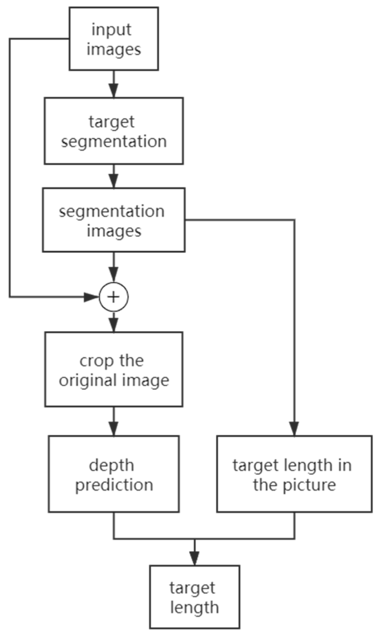
The binocular vision theory simulates the human eye mechanism and estimates the depth through the parallax of the two images collected by left-right cameras. There are several steps for body length estimation. Firstly, the camera is calibrated to eliminate image distortion. The corrected image is segmented by the FCN segmentation algorithm, and the object region will be gathered according to the segmentation map to reduce the image size and the amount of calculation. The distance between the head and tail pixels of the fish is obtained according to the segmentation map. In the subsequent stereo matching process, pixel matching is performed on the cropped regions of the left and right view images to obtain depth information. Finally, the depth information is used to calculate the object’s body length. The specific technical flowchart is shown in Figure 1.
2.1. Camera Calibration
Camera calibration is an important step for binocular vision-based depth estimation, which determines whether the machine vision system can effectively identify, locate and calculate the depth of the object. The Zhang’s calibration method [16] is adopted, the checkerboard image taken by the camera is used as the reference object, and the coordination relationship between the three-dimensional world to the imaging plane is established through digital image processing and spatial arithmetic operations, then the internal parameter matrix and external parameter matrix of the camera are obtained to perform distortion correction for the collected image.
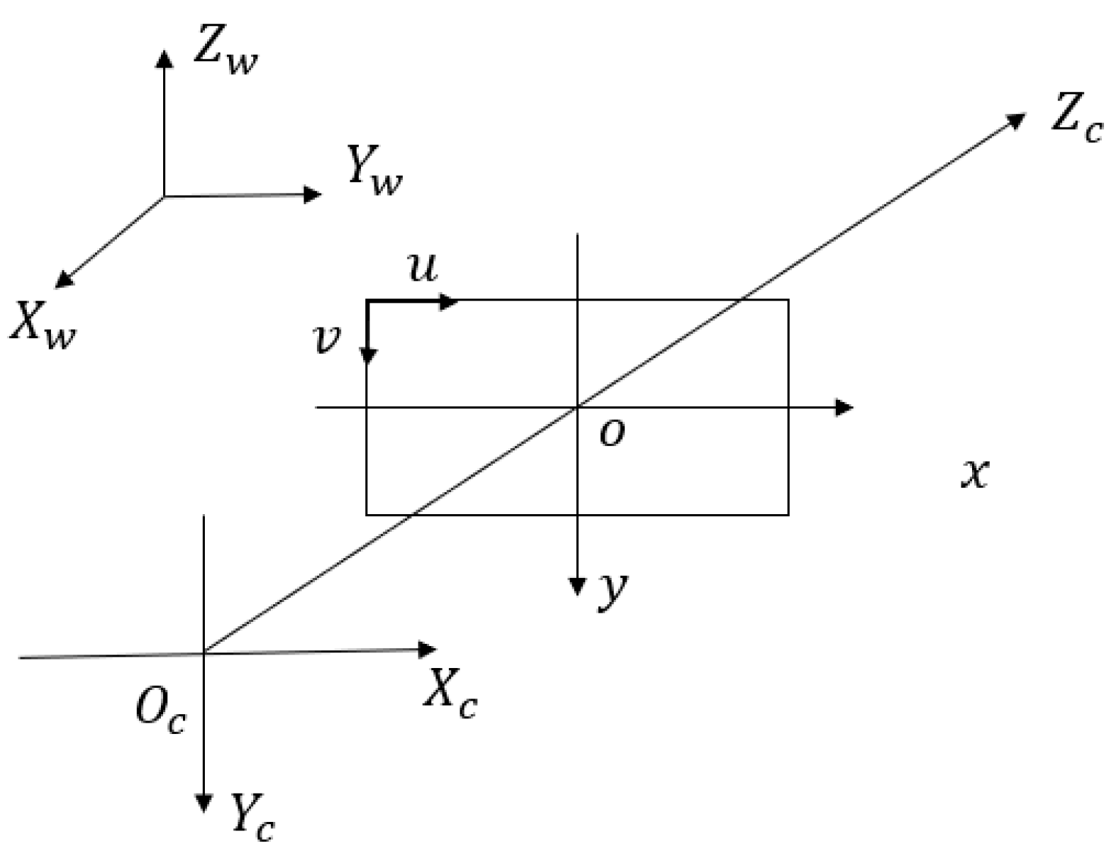
The world coordinate system is , the camera coordinate system is , the image coordinate system is , and the pixel coordinate system is . The mapping among coordinate systems is shown in Figure 2 and expressed as Equations (1)–(3).
where and represent the proportionality coefficient between image coordinates and pixels. is the center pixel coordinate of the image. is the focal length of the camera, is a 3 × 3 rotation matrix, is a 3 × 1 transformation vector. According to the above formulas, the mapping between the world coordinate system and the pixel coordinate system is described as Equation (4).
The internal and external parameters of the camera can be calculated through the mapping. Assuming that the chessboard is at in Zhang’s calibration method, the above formulas can be described as Equations (5) and (6).
is the camera internal parameter matrix, and is a scale factor.
is defined as the combination of the internal parameter matrix and the external parameter matrix. is a 3 × 3 matrix that an element is a homogeneous coordinate, Therefore, there are 8 unknown elements to be solved.
Through the formula , where λ is a scale factor, introducing the constraint condition , the solution of the internal parameter can be expressed as Equations (7) and (8).
There are 5 unknowns in . At least 3 different checkerboard pictures are required to solve these unknowns.
2.2. Fully Convolutional Network
Object segmentation is a method to find specific contour information of the object through a segmentation algorithm. Segmentation algorithms include traditional segmentation algorithms based on threshold [17] and edge detection [18], as well as popular deep learning-based methods including Mask R-CNN [19], FCN [20] and Resnet [21], etc. In this paper, the underwater object data set is adopted to train a fully convolutional network (FCN) to accurately distinguish fish in the image. FCN was proposed by Long et al. in 2015, which is a semantic image segmentation network classifying all pixels of the picture. FCN network replaces the fully connected layer of the convolutional neural network with a convolutional layer, which has two advantages, first, the size of the fully connected layer is fixed, which makes the size of the input image fixed. For a convolutional layer, the size of the input image is not limited. In addition, the output of the fully connected layer is a value to classify the whole image, however, the output of the convolutional layer is a feature map and all pixels in the image can be classified after upsampling.
The main body of FCN is the combination of the convolutional layer and pooling layer alternately, which is used to continuously process a picture and extract features. Generally, it is composed of several parts, and each part includes several convolutional layers with the same kernel size followed by a pooling layer. The convolution layer uses a convolution kernel to traverse the feature map with the corresponding elements. The convolution calculation and image size calculation after convolution are expressed as Equations (9) and (10).
where represent the element value of the output feature map after convolution, is the input value of the convolution layer, and are the parameters of the convolution kernel, which are also called weights. is the bias term. is the size of the original image, and is the step size, which represents the number of interval elements. is the padding layer, which means adding 0 elements to layer around the input image. is the size of the convolution kernel, and is the feature map size after convolution. The pooling layer is used to select the most representative features in the feature map to reduce the number of parameters. The pooling layer generally has two calculation methods, maximum pooling, and average pooling. The maximum pooling is adopted to divide the feature map into multiple regions of the same size, and the maximum value of each region is selected to combine as a new feature map. At the end of each convolution, an activation function is used to remove negative correlation features to ensure that the features are related to the final goal. The Rectified Linear Units (ReLU) activation function is adopted as Equation (11).
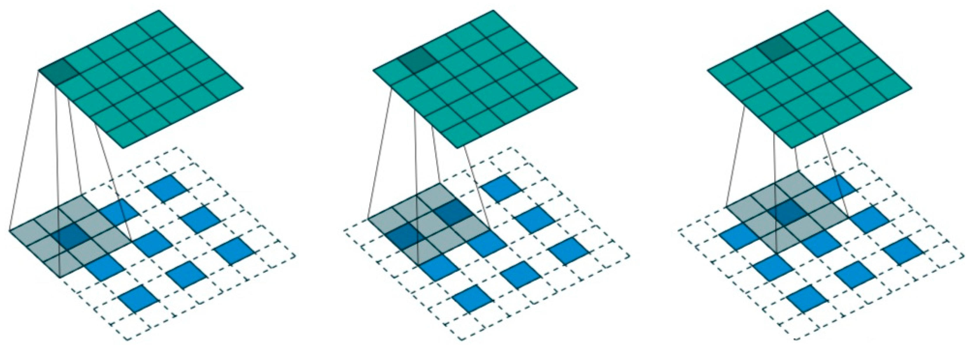
One of the important characteristics of FCN is transposed convolution, which is also called upsampling. The function of transposed convolution is to expand the convolution image to the size of the original image without restoring the original value. The calculation method of transposed convolution is similar to convolution. The image size after transposed convolution is described in Equation (12).
where , , , have the same meaning as convolution operation and is the step size, which means that zero elements are added to the neighborhood. Transposed convolution can be seen as a process of enlarging the feature map and then performing the convolution operation. As shown in Figure 3, a 3 × 3 feature map is expanded into a 5 × 5 feature map through a 3 × 3 convolution kernel after internally filling.
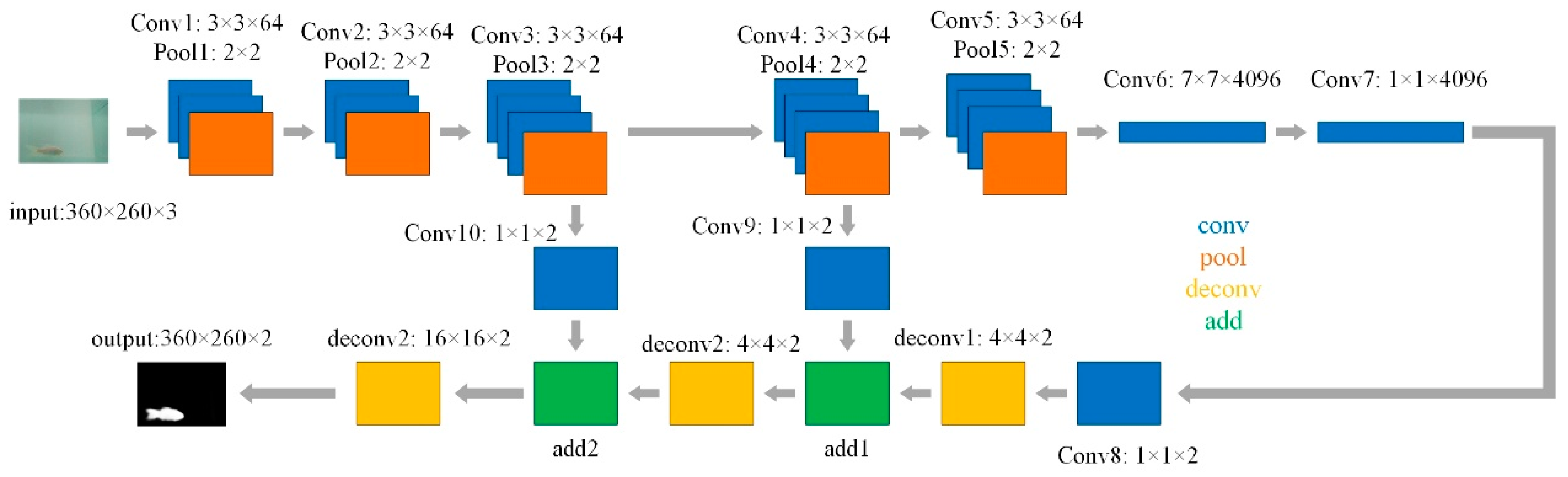
The baseline of FCN is VGG-16 as shown in Figure 4. There are 7 convolutional layers and 5 pooling layers in FCN where the blue block represents the convolutional layer, the yellow block represents the pooling layer, the green block represents the feature fusion layer which sums the corresponding elements with the same dimension, and the orange block represents the transposed convolution layer. The feature map is generated after a series of convolution and pooling operations on the input image. The skip structure is also playing an important role in the FCN. The feature map of the pool4 layer is merged with the feature maps of the pool3 layer to increase the details of the image. Finally, a transposed convolution is used to expand the size of the image as the original image. A softmax is applied to determine the probability of a pixel belonging to a certain class. The feature maps of the third and fourth pooling layers are sequentially added to the conv7′s feature map for taking into account both local and global information.
The 1 × 1 convolution kernel is used to change the number of feature map channels. The feature map after the 7th convolution layer has the same dimensions as the feature map of the 4th pooling layer after the first transposed convolution, and their channel numbers are adjusted to the number of the category. The increased layer fuses the two feature maps by adding elements at corresponding positions. The same operation is adopted to merge the feature map after the third pooling. The feature map is expanded to the size of the original image after the third transposed convolutions.
The segmentation map is used to determine the object region. The region where the object is located is selected, and the irrelevant information is eliminated. The coordinates of the selected regions in the left and right views are used for the subsequent stereo matching algorithm.
2.3. Depth Prediction
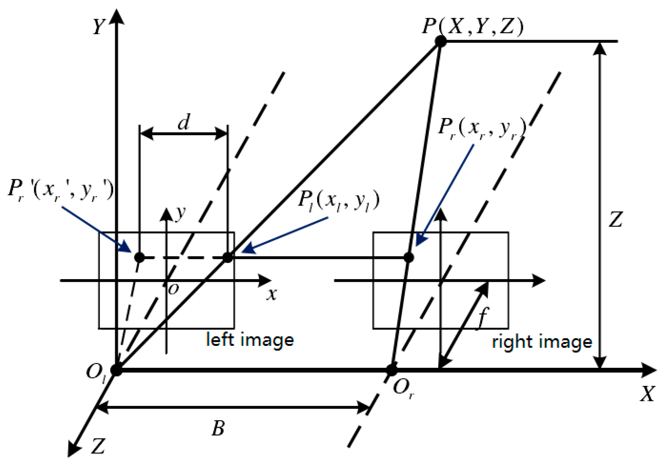
The binocular vision theory is a method to calculate the depth according to the position difference of the same object shot by different cameras based on the parallax principle and is mostly used in three-dimensional reconstruction. Stereo matching is an important technology to find the pixel pair with the highest similarity in the binocular picture. The three-dimensional coordinate system is shown in Figure 5, and represent the positions of the left and right cameras. is the camera focal length, is the pitch of lens, represents the parallax, is the desired distance, and is the pixel of the image. According to the principle of similar triangles, the depth calculation is expressed as Equation (13).
The SGBM [22] algorithm is used to estimate the object depth. The SGBM algorithm is a semi-global matching method that utilizes mutual information for pixel matching and approximates a global two-dimensional smoothness constraint. A global energy function about the disparity map is formed by the disparity of each pixel. The optimal disparity of each pixel is calculated by minimizing this energy function. The energy function is expressed as Equation (14).
where refers to the disparity map. is the energy function corresponding to the disparity map. and represent the pixels in the image; refers to the adjacent pixels centered on pixel , in which usually 8 adjacent pixels around pixel ; The first term refers to the sum of the costs of all matching pixels when the current disparity map is ; The second term adds a constant for all pixels q in the for which the disparity changes 1 pixel, this term is used to adapt to the condition of slightly inclined and curved planes. The third term adds a larger constant for which the disparity changes more than 1 pixel, this term is used to preserve the edge information of the image. It has always to be ensured that . is a logical function, the function returns 1 if the parameter in the function is true, otherwise, it returns 0. There are also parameters such as the initial disparity and disparity range, which can be adjusted accordingly through the segmentation map. The object position difference between the left and right segmentation images can be used as the pre-parallax to constrain the maximum disparity range in the SGBM algorithm.
The solution of the function is an NP-complete problem to find the optimal solution in a two-dimensional image. Therefore, the problem is approximately decomposed into multiple one-dimensional problems which can be solved by dynamic programming. In the algorithm, it is decomposed into 8 one-dimensional problems because one pixel has 8 adjacent pixels.
2.4. Estimation of Fish Body Length
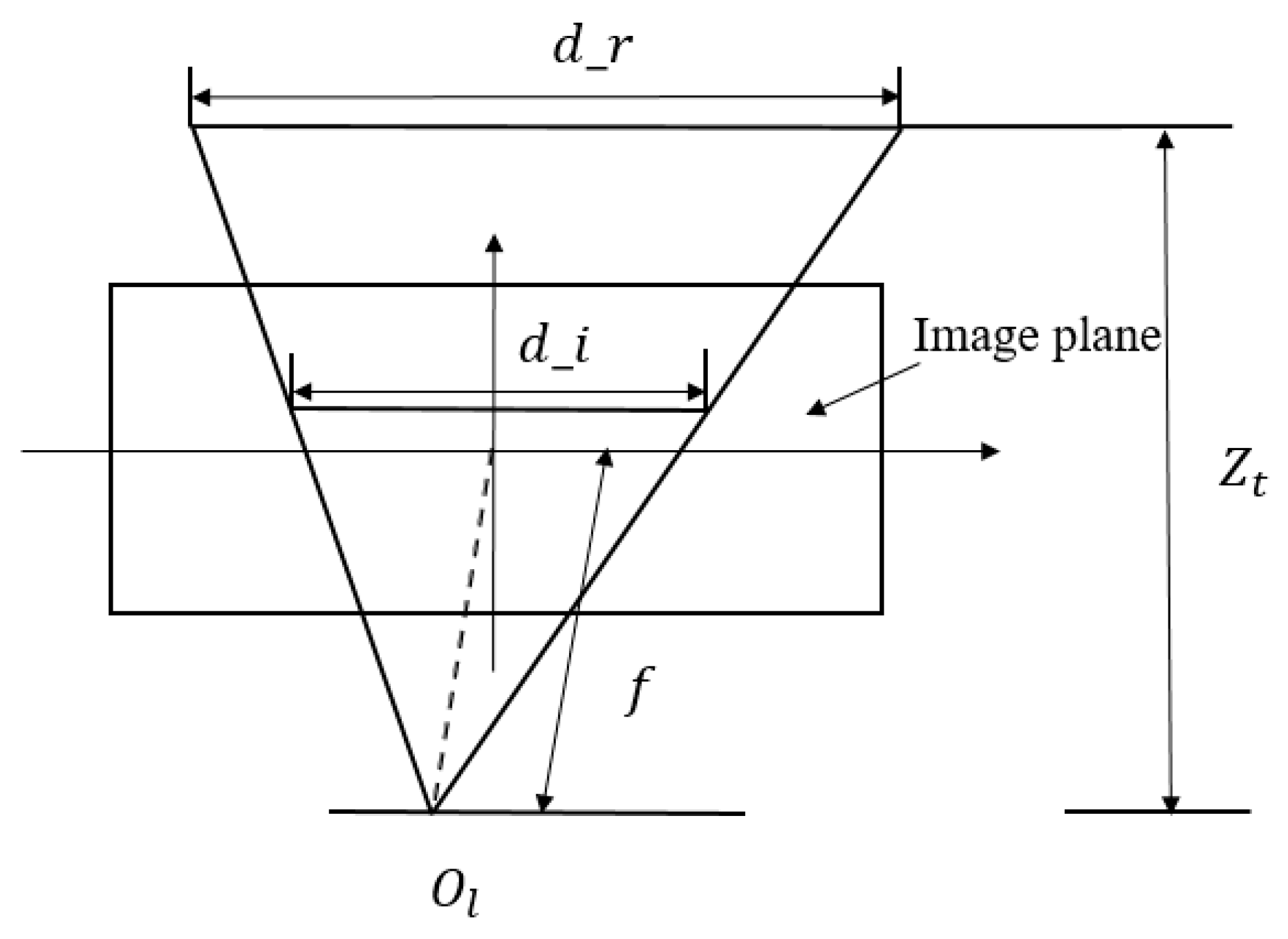
The object body length is calculated according to the coordination corresponding to the object’s head and tail pixels. The head and tail pixel positions of the object are found through the segmentation map, and the depth is calculated based on the disparity map. The corresponding relationship is shown in Figure 6. The fish’s body length estimation is described as Equation (15).
where is the fish body length in the real world, is the focal length, is the fish body length in the image, and is the depth from the camera to the object.
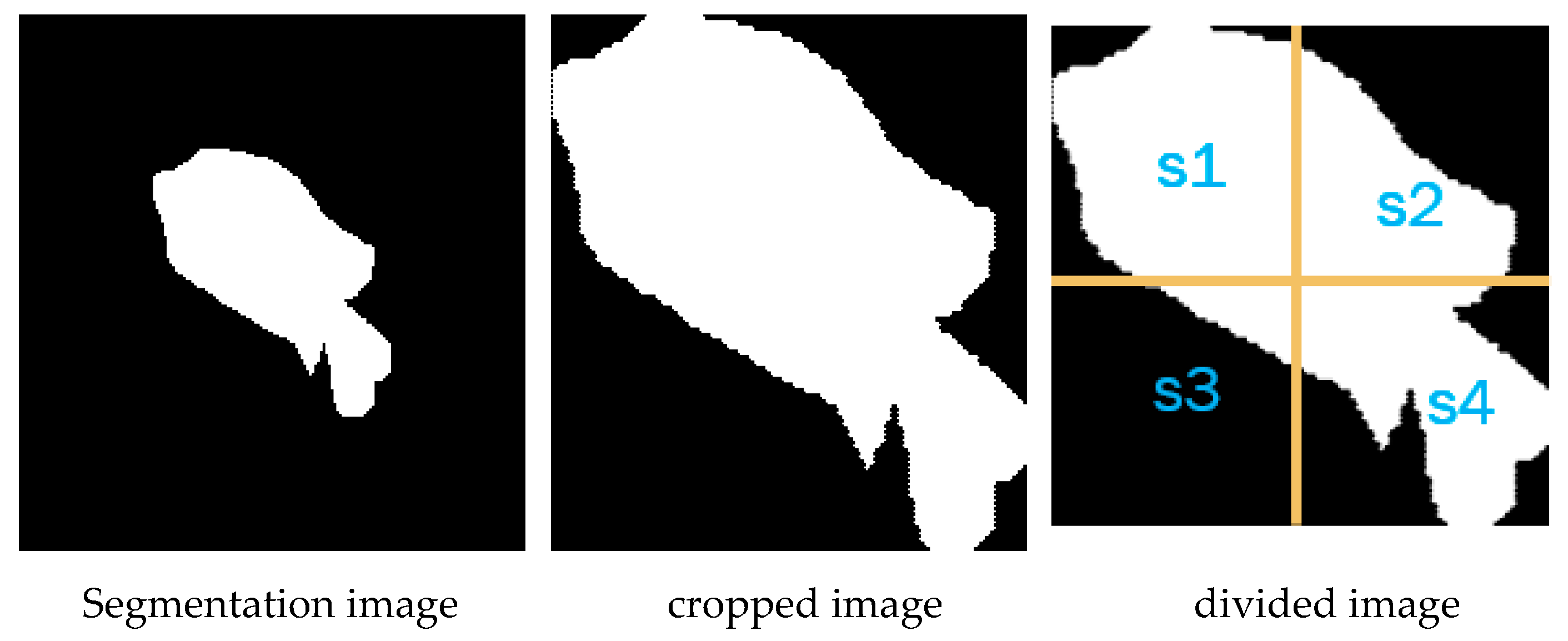
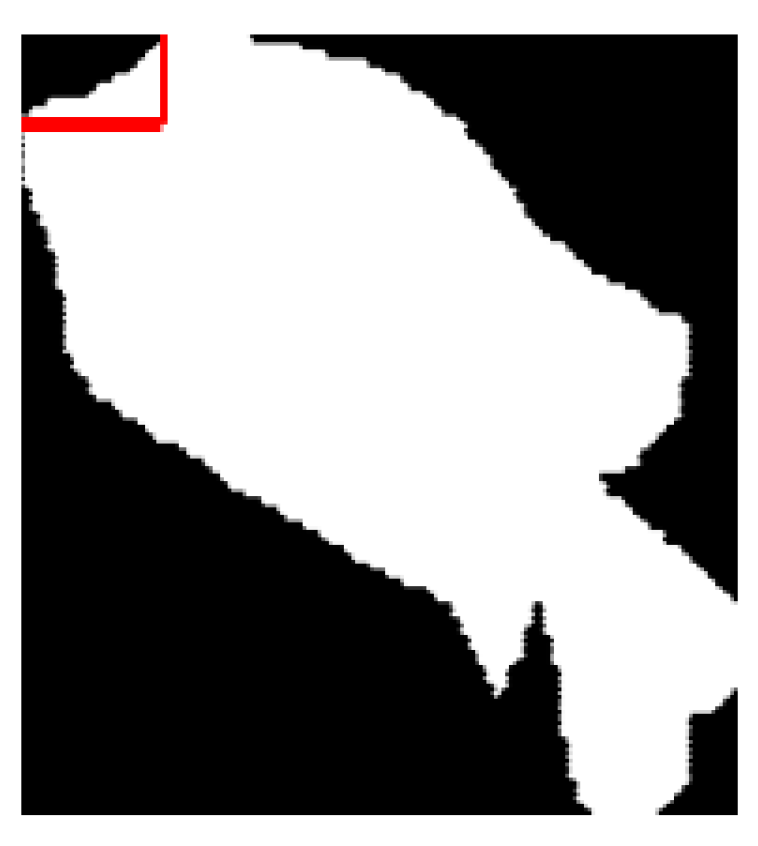
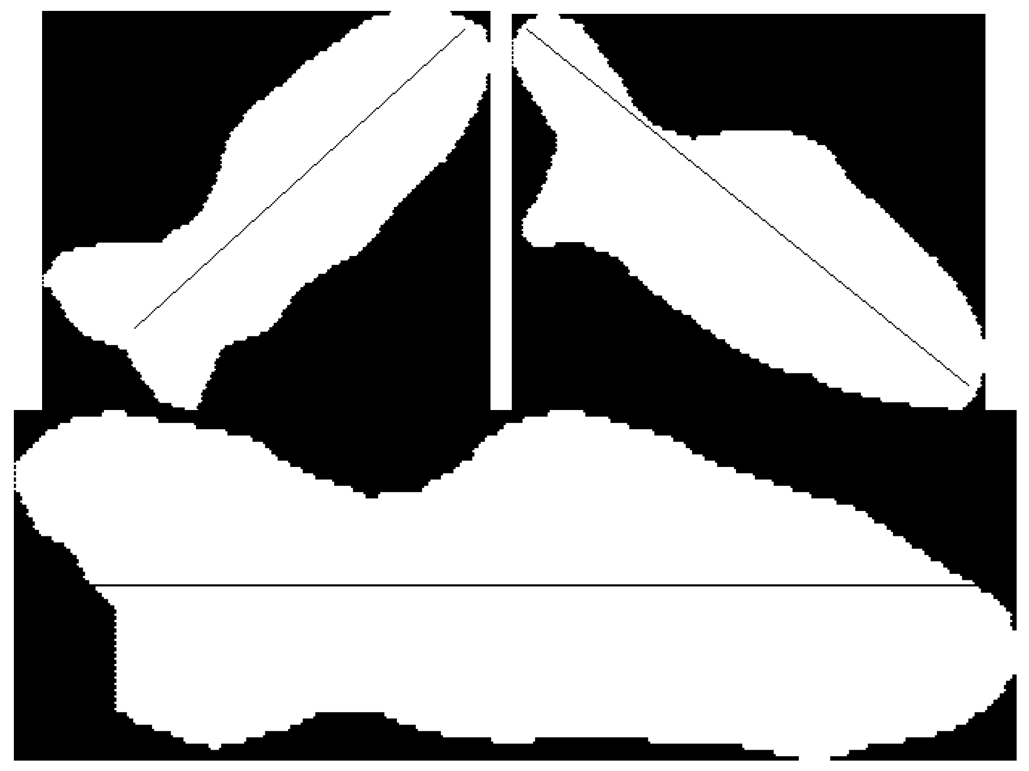
As shown in Figure 7, the object region is extracted based on the edge pixels of the segmentation region. Finding the head and tail of the object is a vital step to estimate the body length. Firstly, the direction of the object is determined. The object orientation is divided into 4 modes, upper-right, upper-left, left–right, and up–down.
The block diagram is adjusted to a square, and then divided into 4 areas with the same size by the centerline. The number of the pixel occupied by the object in the 4 areas are counted as Equation (16), respectively, when the sum of pixels in region 1 and 4 is greater than the sum of pixels in region 2 and 3, the direction of fish is the upper-left, which is expressed as as Equation (17). On the contrary, the direction is the upper-right as Equation (18).
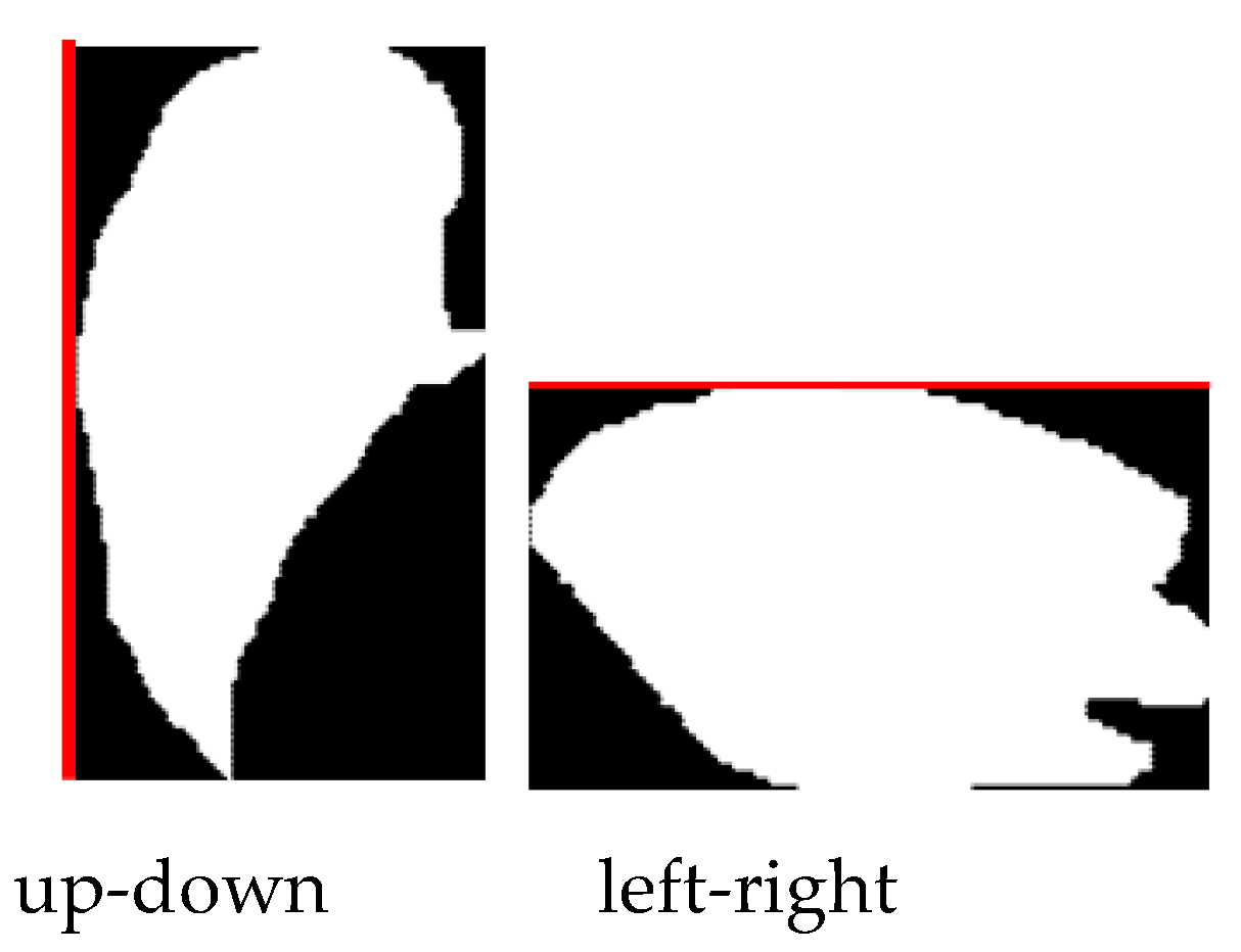
When the sum of the two is not much different, as shown in Figure 8, the long side of the rectangle is defined. If the left side is longer, the direction of the object is up–down as Equation (19). If the right side is longer, the direction of the object is left–right as Equation (20).
Then the head and tail points can be found. As shown in Figure 9, for the left–right orientation object, the midpoint pixel is selected as the head and tail pixel; the same applies for the up–down orientation. For the upper-left object, select the leftmost pixel on the top side of the object and the uppermost pixel on the left of the object, a rectangular region is defined through the two points. The coordinate of the head point is the mean value of coordinates of all pixels belonging to the object in the region as Equation (21). The coordinate of the tail point is found through similar operations for the lower-right region as Equation (22). The same goes for the upper-right object.
3. Experiments
There are few binocular pictures of underwater creatures in the public data sets, so we constructed data sets by binocular cameras. The binocular images were intercepted from the video stream, and the LabelMe software was used to generate a label for the images. There are 200 left and right images. This part of the data was used for FCN and subsequent SGBM algorithms. The amount of data cannot meet the requirements of the deep neural network training, which easily leads to overfitting. Therefore, the underwater fish data set from the fish4knowledge project was adopted for deep neural network training. The fish4knowledge data set was divided into 23 clusters a total of 27,370 pictures, each cluster is represented by a representative species, the species is based on the isomorphic characteristics of the degree of taxa monophyletic. The experimental environment was Linux 16.04, Python 3.5, MATLAB 2019a, GPU TitanX (12G), and OpenCV 4.1.
3.1. Camera Calibration
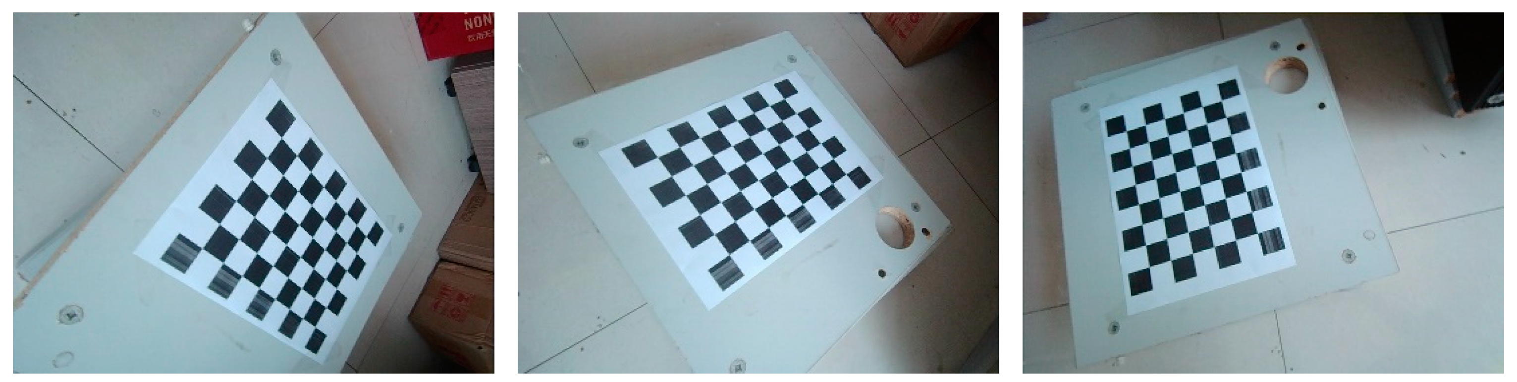
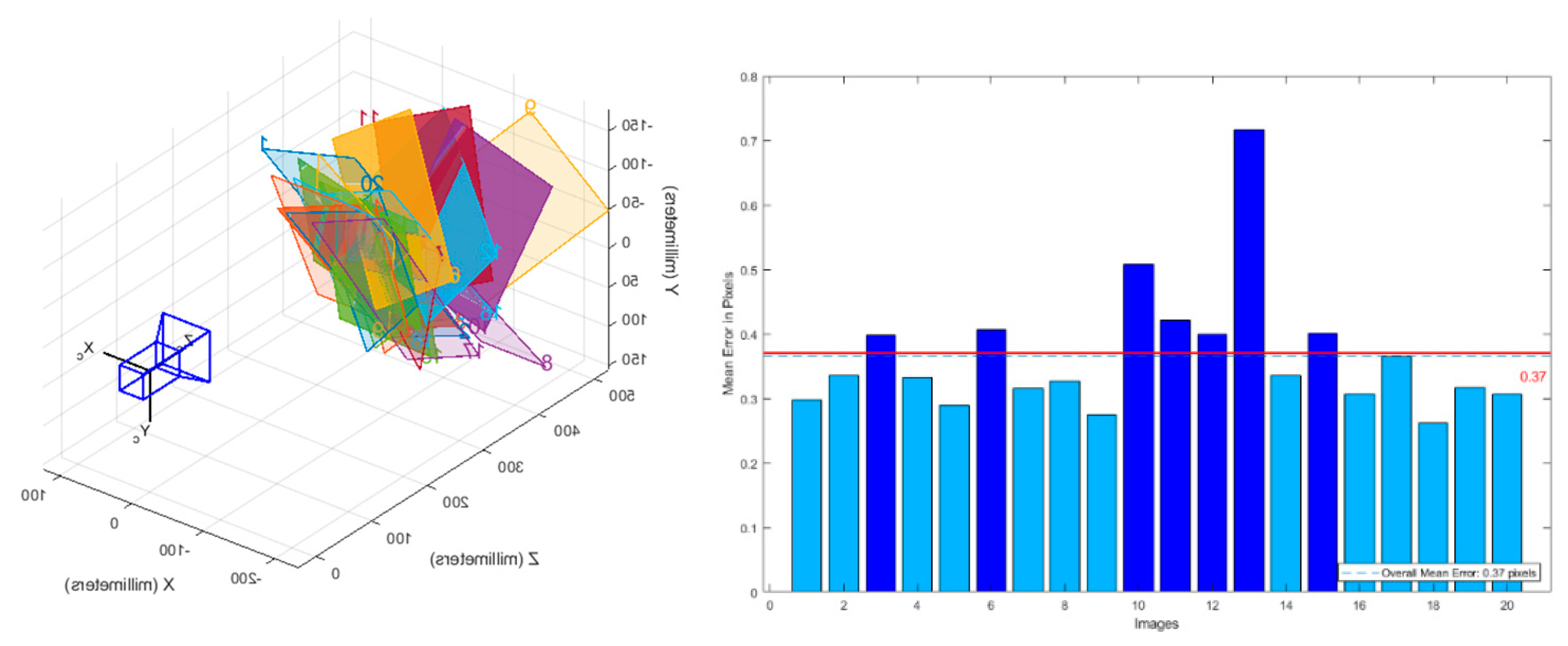
The camera calibration was used to correct the distortion of the image captured by the camera. In the camera calibration process, 20 chessboard pictures were captured. These images were calibrated through the Stereo Camera Calibrator toolbox in the MATLAB 2019a. The calibration board and the result are shown in Figure 10 and Figure 11.
These images are captured at various angles to ensure the accuracy of the calibration. The average reprojection error of most image pixels does not exceed 0.4, and the total average error is less than 0.5, which proves the reliability of the calibration method.
The internal parameter matrices of the left and right cameras are expressed as Equations (23) and (24).
The distortion matrices of the left and right cameras are expressed as Equations (25) and (26).
The rotation and translation matrices between the cameras are expressed as Equations (27) and (28).
3.2. Fish Segment Based on FCN
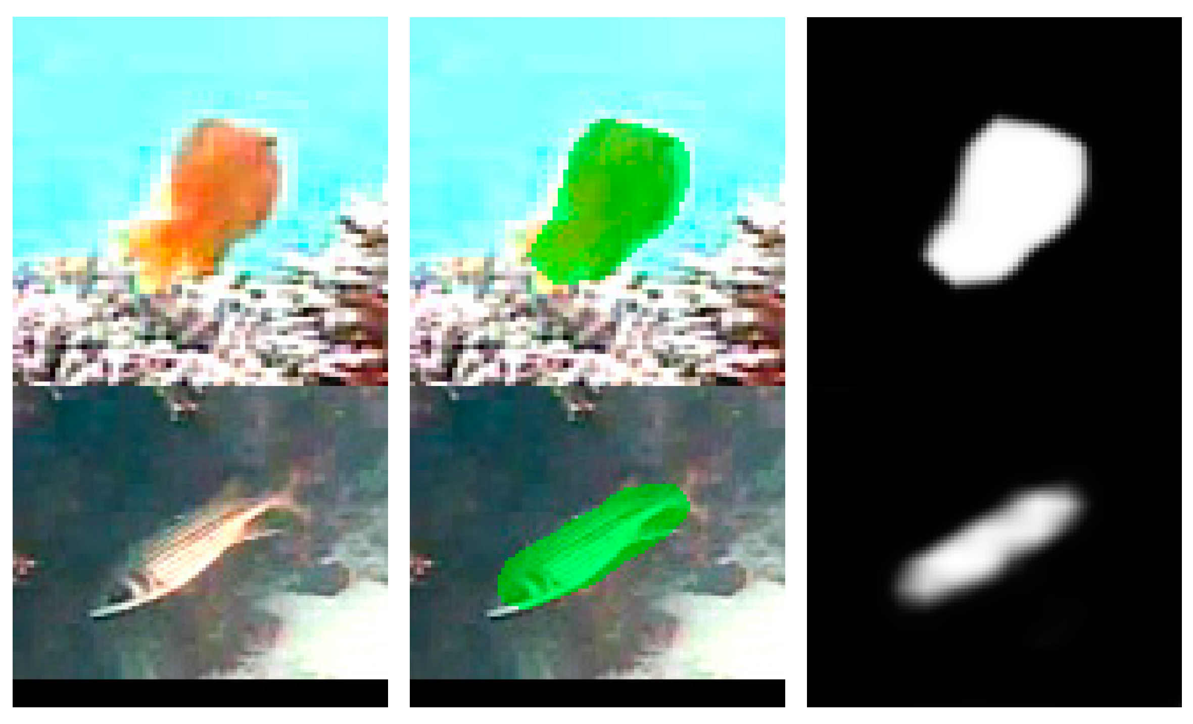
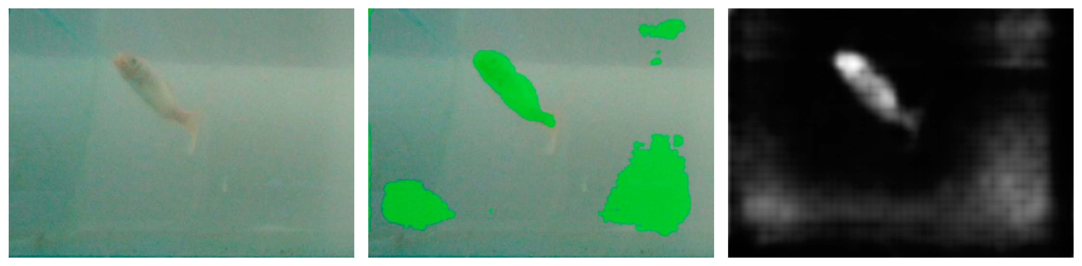
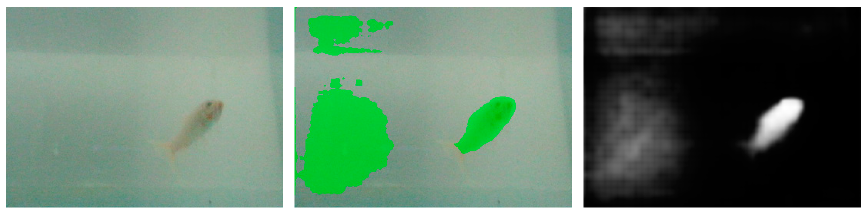
The FCN was trained by the fish4knowledge data set and the performance of the trained model M1 determines whether it can be directly applied to the image segment of a practical binocular camera. The results of the trained model M1 are shown in Figure 12 and Figure 13. Figure 12 is the validation of the model on the fish4knowledge testing data set. The fish can be segmented correctly. The model works well for the fish4knowledge data but does not work well on practical data as Figure 13. The fish coming from the practical data set cannot be segmented. The reason is that the background, the tone, and shape of the fish between the two data sets are different, which makes the model parameters unsuitable. Therefore, the self-made fish data set was added to the fish4knowledge data set for training. The practical data set was used for training to enhance the generalization ability of the model.
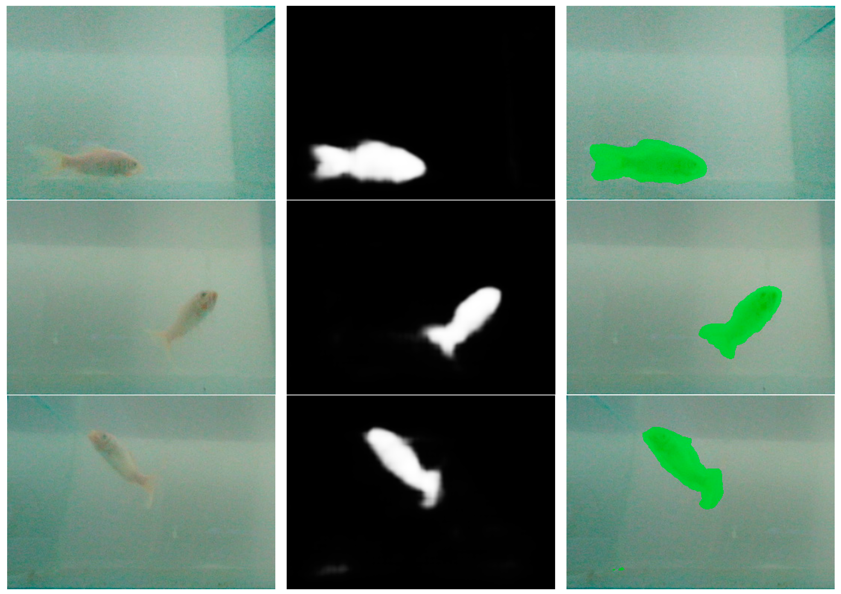
The training data set was constructed using the fish4knowledge data set and the self-made data set; a total of 27,570 pictures were divided into the training set, validation set, and test set with the ratio of 8:1:1. The loss function of the model was the SoftMax cross-entropy, the learning rate was 1e-5, and the number of training iterations was 15,000 to prevent training over-fitting. The results and pictures captured by the camera are shown in Figure 14.
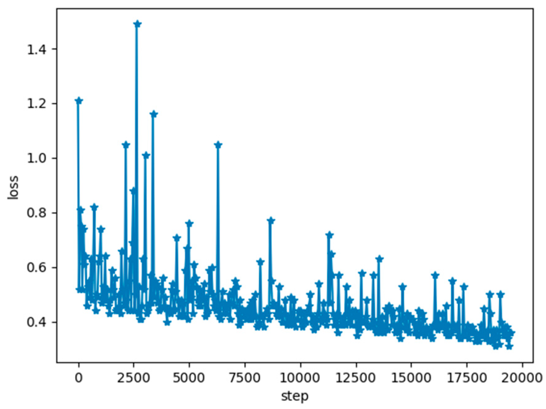
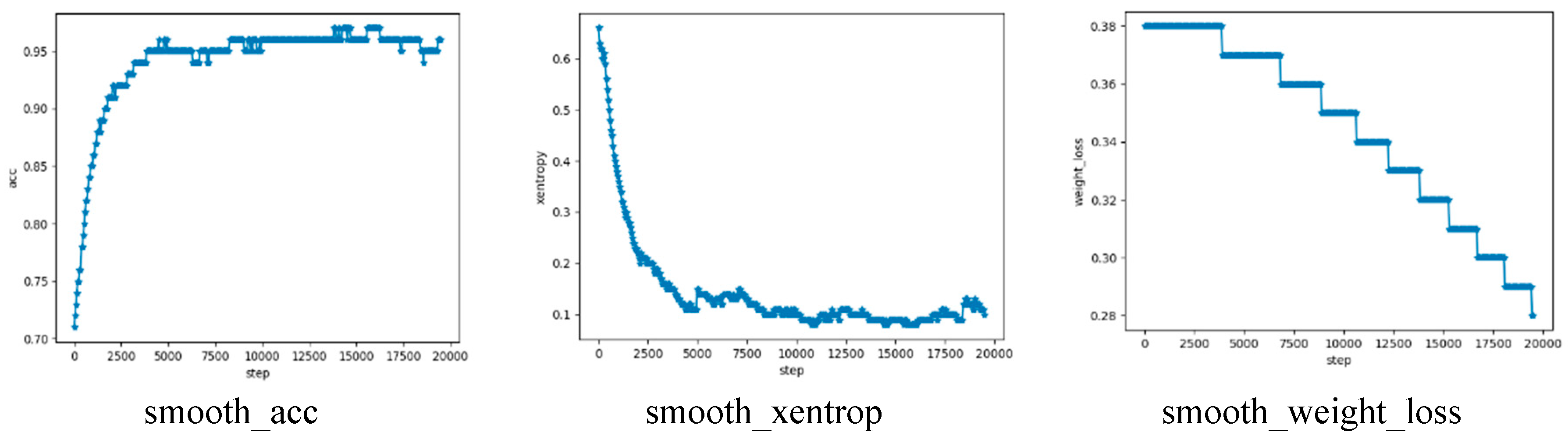
The loss changes during training as seen in Figure 15 and Figure 16. It can be seen that the overall training process is convergent, but there is a phenomenon of a sharp increase in errors at a certain stage. This is because the difference between our data sets was large, and a certain part of the weight during the training process changes may lead to an increase in the segmentation accuracy of part of the image, but a sharp drop in another part of the image. The test result is shown in Figure 16 which represents accuracy, cross-entropy, and weight loss, respectively.
3.3. Depth Prediction
The difference of object position in the left and right images is regarded as a maximum disparity constraint in the stereo matching algorithm. The penalty parameters were set to after multiple experiments, so the disparity map has good performance in the smoothness of the same type and the difference of different types. The sliding window size was adjusted to 7. There were some different filters to preprocess the image to highlight the meaningful characters. Each pixel value in the disparity map represents the disparity of the pixel, and the depth map can be calculated using Formula (2).
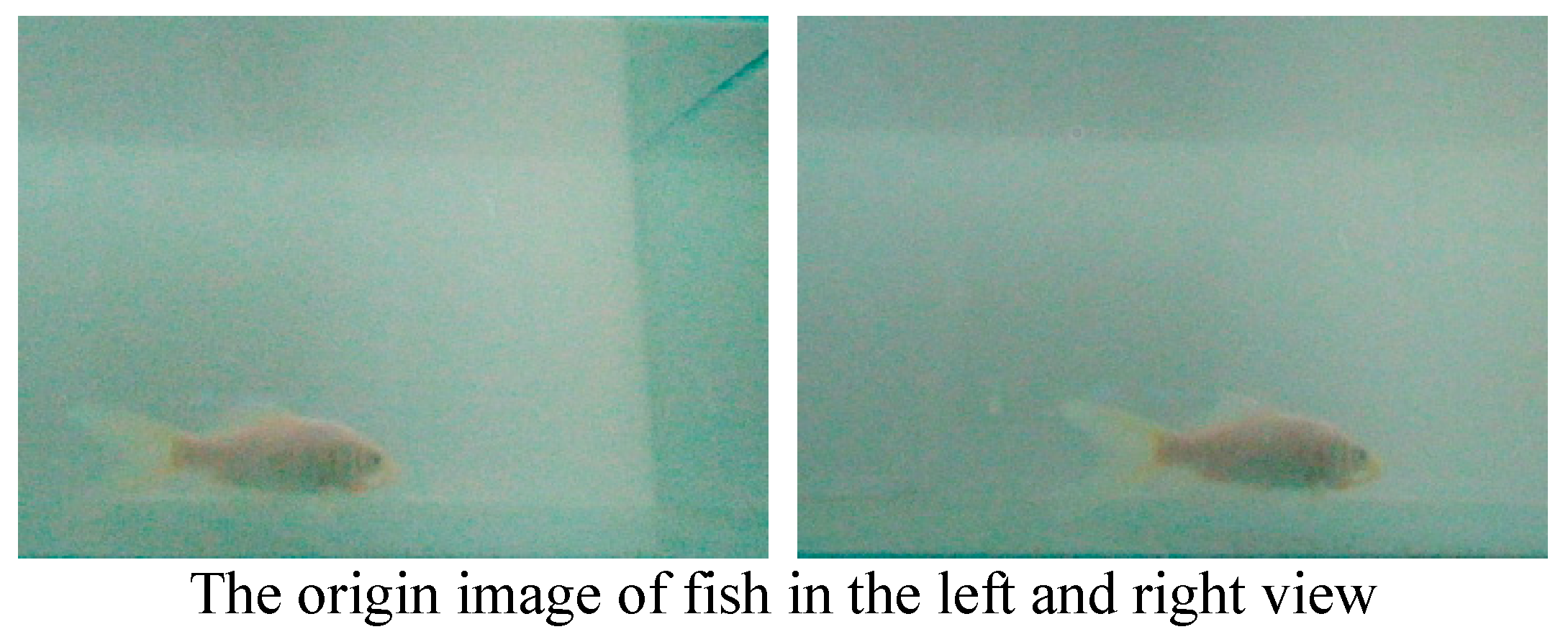
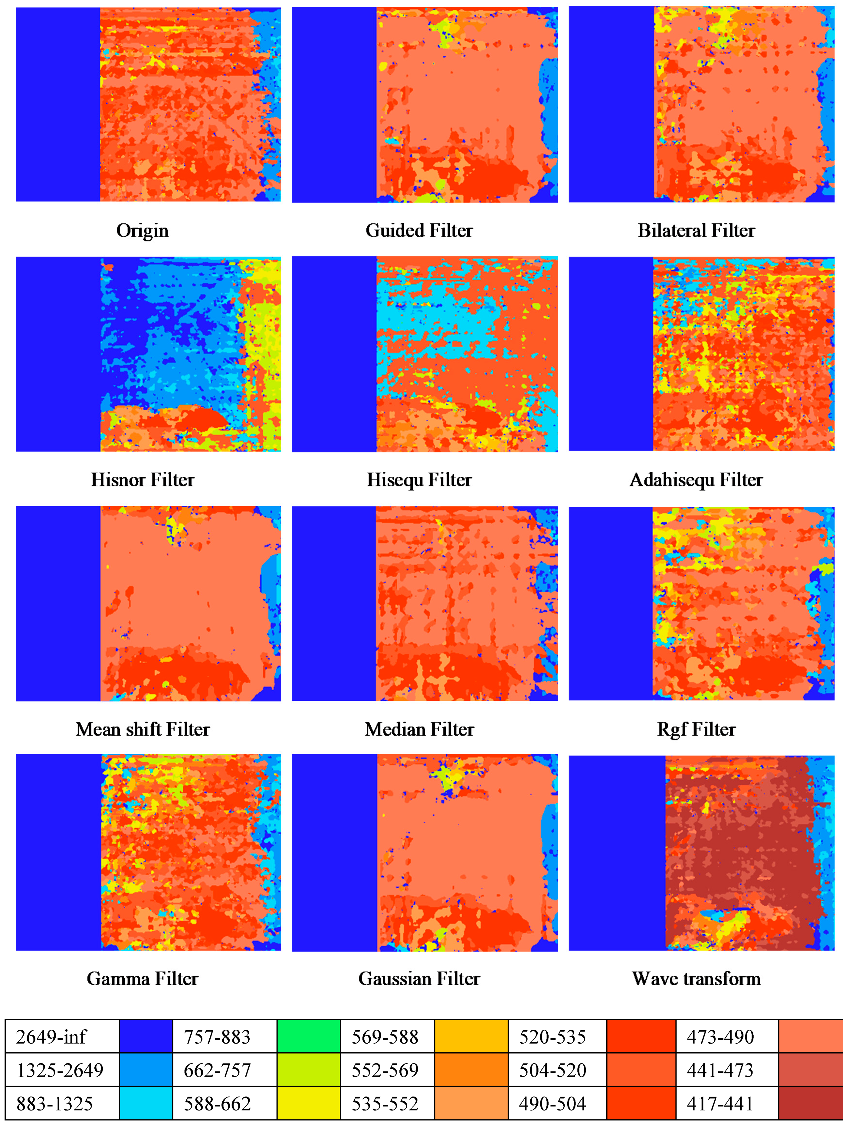
The comparisons of the disparity map between the original image and the preprocessed image are shown in Figure 17 with different colors indication. There are 11 preprocessing methods including Guided Image Filter [23], Bilateral filter, Histogram Normalization, HE (histogram equalization), CLAHE (Contrast Limited Adaptive histogram equalization) [24], Meanshift Filter, Median Filter, Rgf (Rolling Guidance Filter) [25], Gamma Filter [26], Gaussian Filter, and Wavelet Transform. Among them, the performance of Guided Filter, Mean shift Filter, Median Filter, and Gaussian Filter are better. In the general area of the object, the values of the disparity maps are similar, but the object is separated from the background by Guided Image Filter. Therefore, the Guided Image Filter was adopted for preprocessing.
3.4. Fish Body Length Estimation
The body length of fish is estimated according to the position of head and tail. After gathering the position of these pixels, the body length of the fish can be estimated by Formula (3). The body length of the fish in the image is shown in Figure 18.
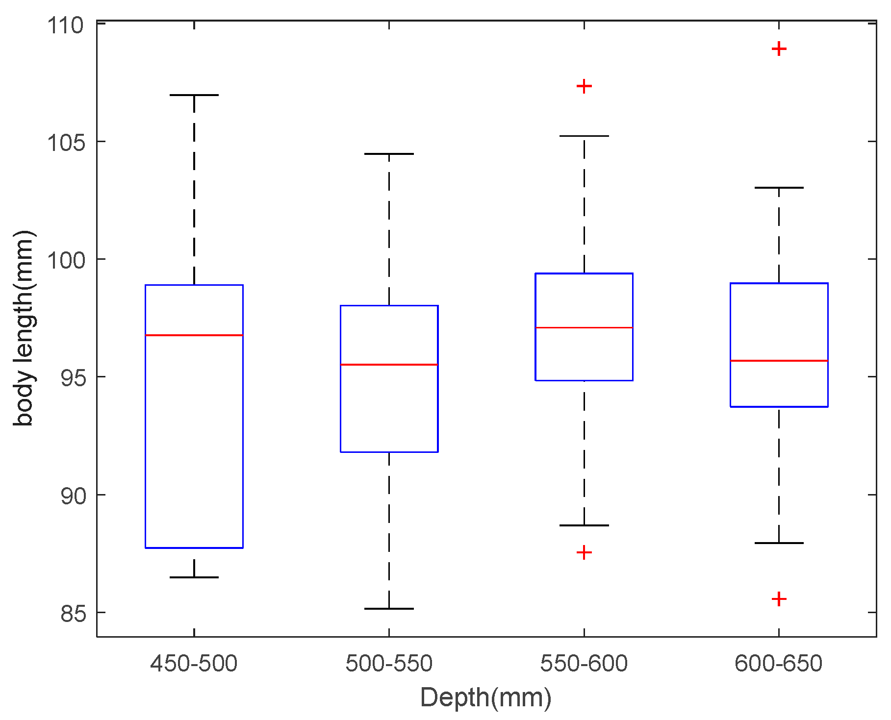
To determine the body length estimation performance of our model, the fish was estimated under different depths, including 450–500 mm, 500–550 mm, 550–600 mm, and 600–650 mm, respectively. The results are shown in Table 1. The actual length of the fish is 10 cm. Table 1 shows the average body length of the estimation at different depths. The error is about 4–5%. The body length estimation accuracy is the highest in the depth of 550–600 mm. The statistics of the results at different depths are drawn in the form of box plots in Figure 19. According to the figure, the results at the depth of 550–600 mm are the most accurate.
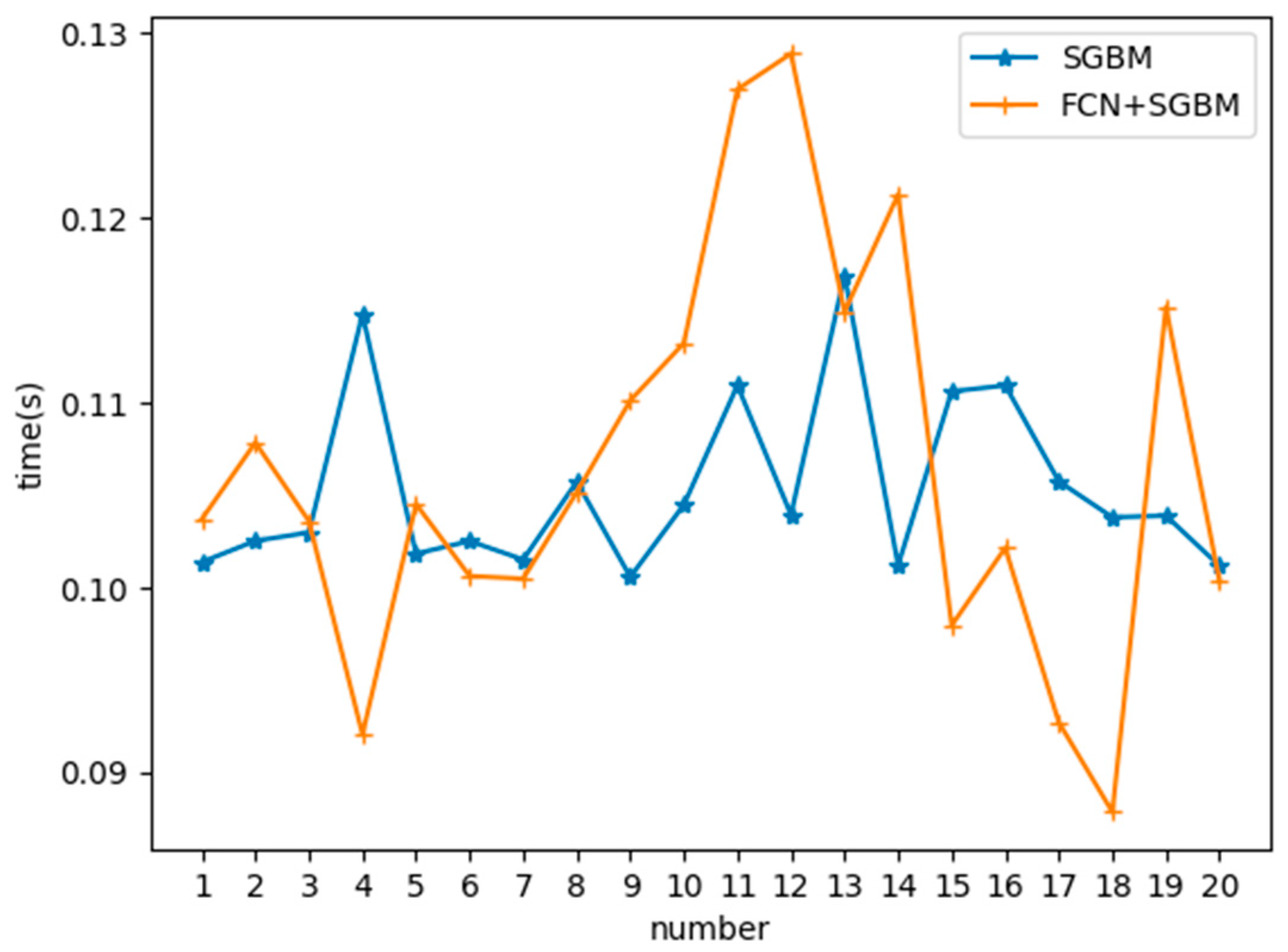
The original SGBM cannot detect the fish. Therefore, it cannot estimate the body length of the fish. A comparison of computation was carried for the disparity map calculation. The SGBM should calculate the whole depth of the image to generate disparity map aimlessness, and the proposed model should do an object segment to generate the disparity map of the object region. A total of 20 samples were randomly selected, and each sample was tested 10 times for a mean value. The final result is shown in Figure 20. For the SGBM algorithm, the time consumption for each pair of pictures is between 100 ms and 120 ms. The proposed algorithm estimates the body length of the fish with 90–130 ms. The fluctuation of time consumption is largely due to the different size of the object region. According to the experiment, the time consumption of the two algorithms is comparative.
4. Conclusions
Aiming at the refine-grained analysis of underwater creature, a body length estimation algorithm combining image segment and stereo matching was proposed. The FCN segmentation algorithm was used to find the specific object region in the image. The SGBM algorithm was used to generate the disparity image of the segment region of the object. The object body length can be calculated according to the disparity map and the object position. The algorithm can be applied to underwater creature detection and reduce the amount of depth estimation computation. At the same time, the accuracy is also improved by the pre-parallax. The optimization of the stereo matching algorithm and multi-objective matching will be our future work to improve the accuracy, speed, and generalization ability of the algorithm.
Author Contributions
Conceptualization, R.C. and Q.X.; methodology, R.C.; formal analysis, C.Z., G.L. and J.S.; writing—original draft preparation, R.C.; writing—review and editing, R.C. and Q.X.; supervision, Q.X.; project administration, Q.X.; funding acquisition, Y.S. and X.Y. All authors have read and agreed to the published version of the manuscript.
Funding
This research was funded by the National Natural Science Foundation of China under Grants (61573213, 61803227, 61603214, 61673245), National Key Research and Development Plan of China under Grant 2017YFB1300205, Shandong Province Key Research and Development Plan under Grants (2018GGX101039, 2016ZDJS02A07), China Postdoctoral Science Foundation under Grant 2018M630778, the Fundamental Research Funds for the Central Universities(2019ZRJC005) and educational and teaching research of Shandong University (Z201900).
Conflicts of Interest
The authors declare no conflict of interest.
References
- Recuero Virto, L. A preliminary assessment of the indicators for Sustainable Development Goal (SDG) 14 “Conserve and sustainably use the oceans, seas and marine resources for sustainable development”. Mar. Policy 2018, 98, 47–57. [Google Scholar] [CrossRef]
- Pauly, D.; Zeller, D. Comments on FAOs State of World Fisheries and Aquaculture (SOFIA 2016). Mar. Policy 2017, 77, 176–181. [Google Scholar] [CrossRef]
- van Hoof, L.; Fabi, G.; Johansen, V.; Steenbergen, J.; Irigoien, X.; Smith, S.; Lisbjerg, D.; Kraus, G. Food from the ocean; towards a research agenda for sustainable use of our oceans’ natural resources. Mar. Policy 2019, 105, 44–51. [Google Scholar] [CrossRef]
- Garcia, R.; Prados, R.; Quintana, J.; Tempelaar, A.; Gracias, N.; Rosen, S.; Vågstøl, H.; Løvall, K. Automatic segmentation of fish using deep learning with application to fish size measurement. ICES J. Mar. Sci. 2019, 77, 1354–1366. [Google Scholar] [CrossRef]
- Salman, A.; Siddiqui, S.A.; Shafait, F.; Mian, A.; Shortis, M.R.; Khurshid, K.; Ulges, A.; Schwanecke, U. Automatic fish detection in underwater videos by a deep neural network-based hybrid motion learning system. ICES J. Mar. Sci. 2019, 77, 1295–1307. [Google Scholar] [CrossRef]
- Spampinato, C.; Chenburger, J.; Nadarajan, G.; Fisher, B. Detecting, Tracking and Counting Fish in Low Quality Unconstrained Underwater Videos. In Proceedings of the Third International Conference on Computer Vision Theory and Applications, Madeira, Portugal, 22–25 January 2008; pp. 514–519. [Google Scholar]
- Lu, Y.; Tung, C.; Kuo, Y. Identifying the species of harvested tuna and billfish using deep convolutional neural networks. ICES J. Mar. Sci. 2019, 77, 1318–1329. [Google Scholar] [CrossRef]
- Sung, M.; Yu, S.; Girdhar, Y. Vision based real-time fish detection using convolutional neural network. In Proceedings of the OCEANS 2017—Aberdeen, Aberdeen, UK, 19–22 June 2017; pp. 1–6. [Google Scholar]
- Mahmood, A.; Bennamoun, M.; An, S.; Sohel, F.; Boussaid, F.; Hovey, R.; Kendrick, G. Automatic detection of Western rock lobster using synthetic data. ICES J. Mar. Sci. 2019, 77, 1308–1317. [Google Scholar] [CrossRef]
- Álvarez-Ellacuría, A.; Palmer, M.; Catalán, I.A.; Lisani, J. Image-based, unsupervised estimation of fish size from commercial landings using deep learning. ICES J. Mar. Sci. 2019, 77, 1330–1339. [Google Scholar] [CrossRef]
- Tillett, R.; Mcfarlane, N.; Lines, J. Estimating Dimensions of Free-Swimming Fish Using 3D Point Distribution Models. Comput. Vis. Image Und. 2000, 79, 123–141. [Google Scholar] [CrossRef] [Green Version]
- Al-Jubouri, Q.; Al-Nuaimy, W.; Al-Taee, M.; Young, I. An automated vision system for measurement of zebrafish length using low-cost orthogonal web cameras. Aquacult. Eng. 2017, 78, 155–162. [Google Scholar] [CrossRef]
- Miranda, J.M.; Romero, M. A prototype to measure rainbow trout’s length using image processing. Aquacult. Eng. 2017, 76, 41–49. [Google Scholar] [CrossRef]
- Viazzi, S.; Van Hoestenberghe, S.; Goddeeris, B.M.; Berckmans, D. Automatic mass estimation of Jade perch Scortum barcoo by computer vision. Aquacult. Eng. 2015, 64, 42–48. [Google Scholar] [CrossRef]
- Abdullah, N.; Mohd Rahim, M.S.; Amin, I.M. Measuring fish length from digital images (FiLeDI). In Proceedings of the 2nd International Conference on Interaction Sciences: Information Technology, Culture and Human, Seoul, Korea, 24–26 November 2009; pp. 38–43. [Google Scholar]
- Zhang, Z. A flexible new technique for camera calibration. IEEE Trans. Pattern Anal. Mach. Intell. 2000, 22, 1330–1334. [Google Scholar] [CrossRef] [Green Version]
- Liu, L.; Huo, J. Apple Image Recognition Multi-Objective Method Based on the Adaptive Harmony Search Algorithm with Simulation and Creation. Information 2018, 9, 180. [Google Scholar] [CrossRef] [Green Version]
- He, Y.; Ni, L.M. A Novel Scheme Based on the Diffusion to Edge Detection. IEEE Trans. Image Process. 2019, 28, 1613–1624. [Google Scholar] [CrossRef] [PubMed]
- Huang, H.; Wei, Z.; Yao, L. A Novel Approach to Component Assembly Inspection Based on Mask R-CNN and Support Vector Machines. Information 2019, 10, 282. [Google Scholar] [CrossRef] [Green Version]
- Long, J.; Shelhamer, E.; Darrell, T. Fully convolutional networks for semantic segmentation. In Proceedings of the IEEE Conference on Computer Vision and Pattern Recognition (CVPR), Boston, MA, USA, 8–10 June 2015; pp. 3431–3440. [Google Scholar]
- Jiang, Y.; Li, Y.; Zhang, H. Hyperspectral Image Classification Based on 3-D Separable ResNet and Transfer Learning. IEEE Geosci. Remote Sens. 2019, 16, 1949–1953. [Google Scholar] [CrossRef]
- Hirschmuller, H. Stereo Processing by Semiglobal Matching and Mutual Information. IEEE Trans. Pattern Anal. Mach. Intell. 2008, 30, 328–341. [Google Scholar] [CrossRef] [PubMed]
- He, K.; Sun, J.; Tang, X. Guided Image Filtering. IEEE Trans. Pattern Anal. Mach. Intell. 2013, 35, 1397–1409. [Google Scholar] [CrossRef] [PubMed]
- Yadav, G.; Maheshwari, S.; Agarwal, A. Contrast limited adaptive histogram equalization based enhancement for real time video system. In Proceedings of the 2014 International Conference on Advances in Computing, Communications and Informatics (ICACCI), New Delhi, India, 24–27 September 2014; pp. 2392–2397. [Google Scholar]
- Zhang, Q.; Shen, X.; Xu, L.; Jia, J. Rolling guidance filter. In Proceedings of the European Conference on Computer Vision, Zurich, Switzerland, 5–12 September 2014; pp. 815–830. [Google Scholar]
- Principe, J.C.; De Vries, B. THE GAMMA FILTER. IEEE Trans. Signal Process. 1993, 41, 649–656. [Google Scholar] [CrossRef]
Figure 1.
Flowchart of object body length analysis.

Figure 2.
Relationship between coordinate systems.

Figure 3.
Transposed convolution.

Figure 4.
Fully convolutional network.

Figure 5.
Depth prediction with a stereo camera.

Figure 6.
Length prediction.

Figure 7.
Estimation of fish orientation.

Figure 8.
Long side definition.

Figure 9.
Head point of the object.

Figure 10.
Chessboard image.

Figure 11.
Calibration results.

Figure 12.
Results of the fish4knowledge project data set on the model M1.

Figure 13.
Results of the self-made data set on the model M1.


Figure 14.
Results on the model M2.

Figure 15.
Loss diagram.

Figure 16.
Accuracy, cross-entropy, and loss diagram.

Figure 17.
Results of filters.


Figure 18.
Length of the object in the image.

Figure 19.
Box plot of results.

Figure 20.
Time in the method of semi-global block matching (SGBM) and combination of SGBM and fully convolutional network (FCN).
Figure 20.
Time in the method of semi-global block matching (SGBM) and combination of SGBM and fully convolutional network (FCN).


Table 1.
The depth and corresponding body length.
| Depth (mm) | Body Length (mm) | Image No. |
|---|---|---|
| 450–500 | 94.9682 | 7 |
| 500–550 | 95.3670 | 10 |
| 550–600 | 96.9442 | 24 |
| 600–650 | 95.8932 | 19 |
© 2020 by the authors. Licensee MDPI, Basel, Switzerland. This article is an open access article distributed under the terms and conditions of the Creative Commons Attribution (CC BY) license (http://creativecommons.org/licenses/by/4.0/).
Share and Cite
MDPI and ACS Style
Cheng, R.; Zhang, C.; Xu, Q.; Liu, G.; Song, Y.; Yuan, X.; Sun, J. Underwater Fish Body Length Estimation Based on Binocular Image Processing. Information 2020, 11, 476. https://0-doi-org.brum.beds.ac.uk/10.3390/info11100476
AMA Style
Cheng R, Zhang C, Xu Q, Liu G, Song Y, Yuan X, Sun J. Underwater Fish Body Length Estimation Based on Binocular Image Processing. Information. 2020; 11(10):476. https://0-doi-org.brum.beds.ac.uk/10.3390/info11100476
Chicago/Turabian StyleCheng, Ruoshi, Caixia Zhang, Qingyang Xu, Guocheng Liu, Yong Song, Xianfeng Yuan, and Jie Sun. 2020. "Underwater Fish Body Length Estimation Based on Binocular Image Processing" Information 11, no. 10: 476. https://0-doi-org.brum.beds.ac.uk/10.3390/info11100476
Note that from the first issue of 2016, this journal uses article numbers instead of page numbers. See further details here.