Using UAV Based 3D Modelling to Provide Smart Monitoring of Road Pavement Conditions


Department of Engineering, University of Palermo, Viale delle Scienze ed.8, 90128 Palermo, Italy
*
Author to whom correspondence should be addressed.
Information 2020, 11(12), 568; https://0-doi-org.brum.beds.ac.uk/10.3390/info11120568
Submission received: 12 October 2020
/
Revised: 14 November 2020
/
Accepted: 1 December 2020
/
Published: 4 December 2020
(This article belongs to the Special Issue UAVs for Smart Cities: Protocols, Applications, and Challenges)
Abstract
:Road pavements need adequate maintenance to ensure that their conditions are kept in a good state throughout their lifespans. For this to be possible, authorities need efficient and effective databases in place, which have up to date and relevant road condition information. However, obtaining this information can be very difficult and costly and for smart city applications, it is vital. Currently, many authorities make maintenance decisions by assuming road conditions, which leads to poor maintenance plans and strategies. This study explores a pathway to obtain key information on a roadway utilizing drone imagery to replicate the roadway as a 3D model. The study validates this by using structure-from-motion techniques to replicate roads using drone imagery on a real road section. Using 3D models, flexible segmentation strategies are exploited to understand the road conditions and make assessments on the level of degradation of the road. The study presents a practical pipeline to do this, which can be implemented by different authorities, and one, which will provide the authorities with the key information they need. With this information, authorities can make more effective road maintenance decisions without the need for expensive workflows and exploiting smart monitoring of the road structures.
1. Introduction
1.1. The Growing Need for Low-Cost Automated Distress Detection Systems
Globally today, road agencies and authorities are facing tremendous difficulties when it comes to making critical maintenance decisions. Road authorities have to plan and implement appropriate pavement maintenance strategies that will allow roads to be kept in a good state. This is important because roads provide access and movement for people, goods and services within a city or community and with poor conditions, key social and economic activities would not be possible [1]. However, constant reductions in road maintenance budgets [2] have limited the scope of these works which have made it more critical than ever to have low-cost systems in place that can provide data to enable good decision-making practices. Additionally, with the future development of smart cities, it will be critical to have smart systems in place for monitoring road systems. Traditionally, agencies have relied on a pavement management system (PMS) to adequately allocate resources for road management in the best possible combination given the financial limitations [3]. The PMS is utilized as a support system for making decisions concerning planning road maintenance strategies.
Pavement maintenance and their related activities and interventions generally refer to activities that can help to slow the deterioration of pavements through pinpointing and targeting of explicit deficiencies and problems that contribute to the overall structure’s deterioration. In many instances in the past and in cases where authorities are under-resourced, a “worst-first” approach to pavement maintenance has been utilized. In this approach, pavements are not treated until they reach a level of high degradation and then major rehabilitation and maintenance are required [1]. To curb this, some agencies have stressed the importance of carrying out cost-effective preservation activities which have spurred the movement towards more preventative and preservative programs that aim to improve safety and mobility to produce longer pavement life cycles [4].
Typically, the final selection of treatments and plans has to assess the needs and constraints of the particular project and city/region but these are all based on the input of current and historical pavement performance data along with data on the maintenance and rehabilitation activities that were carried out in the past [5]. This exemplifies the importance of data and data analyses to the entire process. It also further shows that without accurate or available data, any decisions made can be flawed and result in poor systems that can end up being costly and unsustainable in the long term. To improve the sustainability of the system it is always considered a positive to choose the correct intervention at the right time [6]. Unfortunately, a significant roadblock to the correct implementation is the acquisition of accurate road condition data which can be costly and time-consuming [7]. Because of this, road databases are not kept up to date or are updated using manual surveys that have high levels of subjectivity in them [8]. All of these factors have led to numerous research projects on generating low-cost techniques for the acquisition of road condition data [9,10].
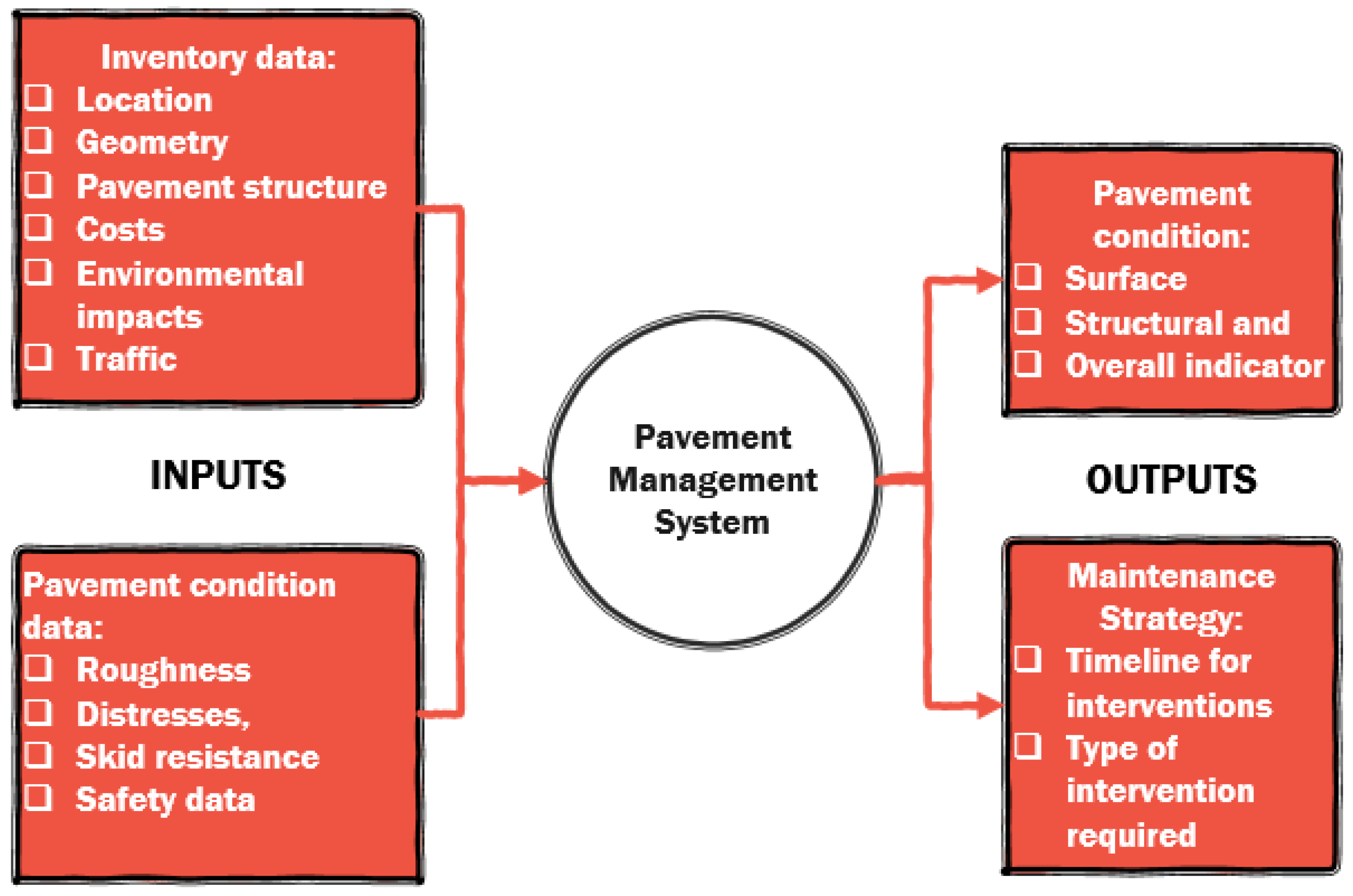
Within the PMS, the data inputs are a vital component. For the road asset database to be effective, the phases of data collection storage and management have to be efficient and cost-effective [11]. Three success factors are designated for the effective management of databases and these are relevance, reliability and affordability [12]. New technologies must adhere to these factors so that their inclusion in the system can be effective and be trusted by road authorities. There are two major categories of data collected for pavements and these are inventory data and pavement condition data. Based on these inputs, information on pavement distresses forms a very important part in defining the condition of a pavement and in identifying the appropriate treatment. The evaluation is typically made of up of three factors: type, severity and extent of the damage. The uses of the data are summarized in Figure 1.
Within the figure, it is shown that the input data is fed into the PMS to yield the outputs of understanding what the conditions are and deciding on the maintenance approaches. It is critical to have systems in place that can produce the required data. However, in many instances, the collection of this pavement condition data is done manually with some studies indicating the number to be as high as 90% of the cases [2], which therefore adds a tremendous amount of subjectivity into the process. This is typically due to the acquisition process of these data being very expensive, exhaustive and time-intensive [7].
1.2. The Current State of Pavement Distress Detection Applications
The equipment utilized for the surveys relates directly to the methods used and the available funds and resources by the road authority. The typical devices per category are listed in Table 1 [9]. However, despite the global availability of these devices, the main approach for detecting pavement distresses is using manual surveys given typical budgetary limitations. Pavement roughness and permanent deformation are typically estimated using static laser sensors that allow the measurement of the longitudinal and transverse profiles of the pavements [13] whilst for all other surface distresses, the most common type of survey is based on the visual evaluation of the defects and the results are affected by subjectivity and high degrees of uncertainty.
Of the areas illustrated in Table 1, the most researched are those based on the use of lasers and imagery. Concerning the laser-based methods, there are numerous commercial applications and systems, which are linked to survey vehicles carrying out surveys across a network. These systems are highly accurate but can be very expensive and would not be obtainable by small or under-resourced agencies or authorities [14]. Many of them are based on the work carried out in the development of the Laser Crack Measurement System (LCMS) [15]. This system utilizes vehicles that are equipped with high-performance lasers that measure road profiles, roughness and slopes at a resolution of 1 mm while simultaneously generating three-dimensional profiles of the pavement. Other applications have considered systems with mobile lasers and light detection and ranging (LIDAR) systems [16,17,18] but their applications have been shown to have issues with deployment and accuracy. There have also been attempts in which both cameras and lasers are utilized in one system to produce road condition data featuring images and profiles from laser profilers [19,20].
Typically, the laser-based systems offer the greatest accuracy amongst the methods but given their associated high costs, image-based systems are often seen as the more appealing option for many studies and subsequent implementations. Most image-based systems utilize cameras equipped to vehicles which survey a road or network and capture images throughout the survey. The images are then utilized in various detection systems using different algorithms and techniques [13,21,22] to identify the distresses present on the road along with the location and associated severity levels.
Previous studies have utilized image-based systems and techniques to detect, classify and analyse pavement distresses [23]. Other studies have also applied deep learning and artificial intelligence to automatically detect distresses [24,25,26]. Of particular interest recently is the use of a stereoscopic based method, which utilizes photogrammetry and structure-from-motion. Using the techniques, three-dimensional (3D) models of pavement sections can be made with the use of regular two-dimensional (2D) images from cameras. Recent studies have been able to use this method to accurately replicate pavement distresses and they have demonstrated the capacity of the method to be utilized in the further steps of analysis and database generation for road authorities [27,28]. With the consideration of this modelling approach, it has also been demonstrated that the methods can provide the required metric information to satisfy industrially recognized distress manuals and also produce additional pieces of data such as volumetric deviations of the surface. It has also been shown that the information required by authorities varies based on the location and specific situational context, as distress manuals vary significantly in terms of the measurement and type of the distresses present so every approach needs to be adjusted based on the actual network conditions [29]. Based on these advances, this study aims to take the research further to examine the practical uses of the data produced and further build the pipeline with new segmentation algorithm applications and over a longer test section, therefore, better imitating a real-world application.
1.3. The Rising Use of 3D Image-Based Modelling and Drones to Detect and Analyse Pavement Distresses
As previously mentioned, structure-from-motion (SfM) is a modelling technique which is used to generate 3D models of objects using 2D images. Algorithms are used for the reconstruction of the required object using overlapping 2D images [30,31]. The images are captured during surveys of the required object in which the camera is directed at points across the object with an overlap of approximately 70%. Once the images are captured, algorithms are then used to align the images in space and then a bundle adjustment process is done to locate where the object is in a 3D space. This is aided by markers or ground control points, which allow the model to be metrically accurate. Figure 2 displays an example dataset of a short survey of an asphaltic pavement section. The blue rectangles in the image represent the overlapping position of the camera at each point of image capture during the survey.
Historically, the primary focus and use of SfM techniques have been in the field of architecture, cultural heritage and archaeology, where models are generated to help preserve data and models of artefacts and important historical buildings [32,33]. Older studies have considered the use of the techniques for road condition monitoring and evaluation [34,35,36] but criticisms arose which included inadequate accuracies and exhaustive computational power. Recently, some of these shortfalls have been solved with the advancements of available software that utilize algorithms with the ability to process models quicker with proven higher accuracy levels. This has made it possible for the applications in pavement engineering to be appropriate [27].
The use of drones to carry out image surveys has also been considered in previous works and applications of inspections of civil infrastructure [37,38]. This is due to the ability of drones to cover a wide area without having to have direct interaction with elements of the pavement structure. Furthermore, by using current marketplace drones it is possible to obtain images with high resolutions that result in data archiving done in shorter lengths of time and at lower costs than traditional approaches. Given these reasons, other studies have utilized them for observing pavement conditions [18,39,40,41]. Particular studies have also used the imagery to generate maps and measure the precise deformations of potholes and rutting [42,43]. Notwithstanding these advantages, there are also limitations with the general use of drones which include inclement weather (rain and wind obstructions), interferences with obstacles near the road (such as trees and buildings) and legal aspects which can forbid or limit the use of a drone in particular areas or communities. Additionally, when carrying out image surveys using drones, there needs to be limited traffic and the surveys have to be done during daylight. Whilst these limitations do present a challenge to some applications using the device, there is still tremendous potential especially for authorities who have limited data and who can ensure that the legal regulations are in place to carry out the surveys. Surveys can also be carried out quickly in periods with limited traffic to help avoid some of the previously mentioned limitations.
The primary focus of many studies using drones has been in the area that can be covered by drones and how techniques can be used to generate a 3D model of the road structure. However, this study attempts to take the process further, identifying how the information should be processed and utilized by the authority to help manage pavement maintenance systems and programmes and better monitor the conditions of the road networks. Furthermore, previous studies have focused on small sections of roads and have used the techniques at specific points of interest, whereas this study considers taking images in a continuous manner along the grade of the road establishing the possibility of modelling a full road section.
1.4. Utilizing Segmentation to Analyse 3D Models of Pavement Sections
Once the SfM techniques are utilized, the generated 3D models can be used to analyse the road conditions. To do this, methods are needed to recognize features and patterns within the replicated models. One method to do this is using image segmentation. This involves dividing the image or model into smaller sections or parts based on similar features or characteristics. This can be done with pavement models to segregate and then subsequently analyse the distresses present in the pavement section. Several data sources have been used to segment images and models, which include:
The data acquisition can be expensive in many of these instances, which can be a deterrent to using the process in practical scenarios. Additionally, the segmentation techniques can be overly complex which makes their use harder as significant training would be required for practitioners to apply the techniques. Consequently, this study aims to develop a low-cost workflow using drone imagery, which can be used to get quick overviews of the sections of a road network.
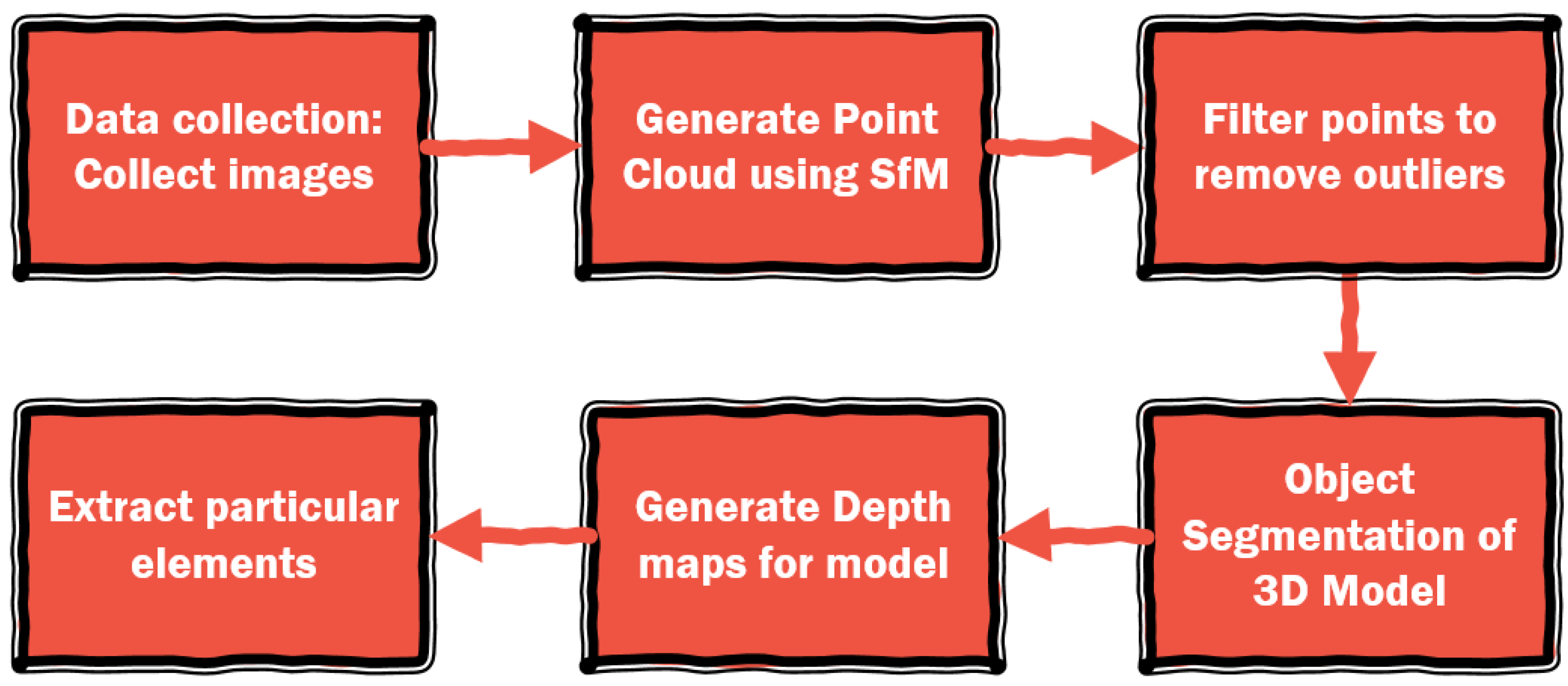
Using the imagery obtained from a drone survey, SfM techniques can be applied and then used simultaneously with the segmentation techniques to isolate the pavement distresses. The SfM technique produces a point cloud which can be classified and then subsequently used to generate depth maps and subsections of the models [51] which explain the deformation of the pavement section. The generic process of segmentation is in illustrated in Figure 3.
Using the generic outline, this study attempts to segment the models from the SfM process using drone imagery and generate depth maps and isolated subsections, which can be used to explain the road condition in terms of deformation and roughness.
1.5. The Specific Aim of the Study
Given the issues raised with automated methods needed for detecting pavement distresses, this study aims to address these problems by generating 3D models of the pavements through the use of unmanned aerial vehicles. To this end, a case study is used where a pavement section is surveyed using a drone to capture images along the pavement’s surface. Once the data is collected, 3D modelling is carried out, followed by the use of segmentation techniques and analysis to give a metric breakdown of the pavement’s condition. A flexible pipeline is established that can be replicated in a practical environment to boost the information available to a road authority without the use of expensive vehicular surveys or subjective manual ones. The output provides another step towards automating aspects of the data collection system at a low-cost.
2. Materials and Methods
2.1. Structure-From-Motion Technique and Pipeline
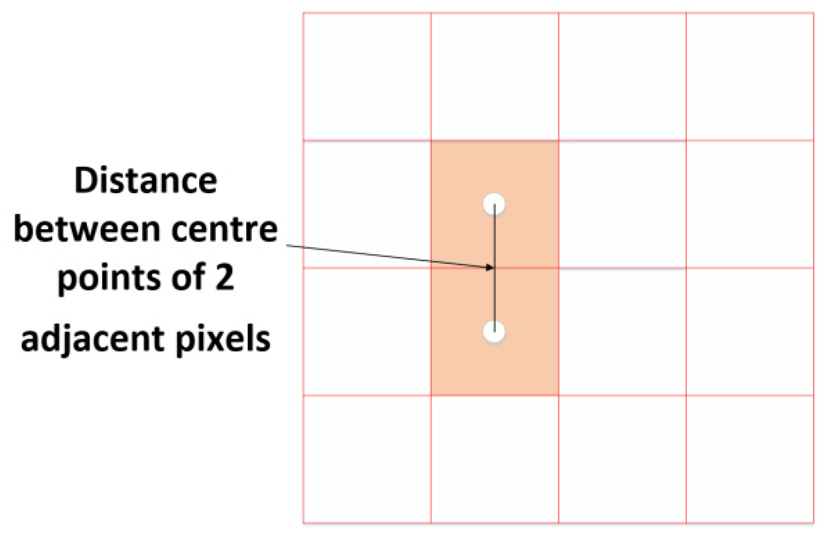
When using 3D modelling techniques based on structure-from-motion, the most important parameter to be understood and quantified in surveys is the ground sampling distance (GSD). This is because this is the parameter from which models are interpreted. The GSD is the distance between two consecutive pixel centres, with respect to the real ground measurements as shown in Figure 4.
Furthermore, it details the smallest observable objects within the image and subsequently the replicated model [52]. The greater the value of the GSD is, the fewer details are measurable. Therefore, it important to understand the size of details that are required in a survey and the subsequent final model. The GSD will provide the resolution of the generated models. The size of the smallest visible details should generally be two to three times the value of the GSD during the survey [53]. This means that it will not be possible to accurately measure and decipher any details on the model that have a real-world measurement that is smaller than 2–3 times the value of the GSD. Given this, it is important to establish what measurements are required for typical pavement distresses. In past studies, it has been shown that the most common distress severities are generally no smaller than 10 mm [54]. For other studies, related to this, a 3 mm resolution is utilized which corresponds to the metric values of distresses within global survey manuals [10]. Given this, and using the rule of thumb previously identified, if a resolution of 3 mm would be enough to identify and analyse these distresses then a GSD one-third of this value would be sufficient for the survey. Therefore, the GSD should have a value no larger than 1 mm. This is however a benchmark and if the actual GSD is lower, then the smallest details would be more visible and the models more clearly represented. The GSD is related to the camera parameters and is given by Equation (1) below:
where D = object distance, ƒ = focal length and pxsize = pixel size (as defined by the ratio of the camera’s sensor size to the image size). The camera parameters of focal length and pixel size can be adjusted to yield an appropriate GSD. For this study, a GSD of 1 mm was aimed for based on the requirements seen in previous work linking industry standards to models [28]. With this GSD in place, the resolutions of the resulting model would allow measurements to be made that could explain the severity assessments of the distresses present on the pavement. Given this, the object distance was manipulated to ensure this value was obtained for the survey. Based on this the equation could be rewritten as shown in Equation (2) with the focus on the object distance:
The object distance will not remain exactly constant during the surveys but an approximate value should be determined beforehand which surveyors should try and not exceed during the survey. To apply Equations (1) and (2), the internal parameters of the camera have to be considered. For the survey, the commercially available DJI Mavic 2 Pro drone was used for the surveys (Figure 5). The cost of this drone or one with similar specifications is negligible in comparison to the cost of a survey vehicle equipped with lasers and other tools.
The specifications of this device are given in Table 2, which includes the exact camera specifications utilized for the surveys. The weight is particularly important as this is a dimension that is consistently mentioned in regulations and must be adhered to in order to allow for flights.
Given the specifications of the camera, the object distance was calculated. This resulted in a required object distance of 11.81 m to produce the associated GSD value. Given this value, it was then decided to survey a maximum flying height of 10 m to ensure that at no point the object distance exceeded the recommended value. This was done by monitoring the altitude of the drone throughout the survey with respect to the ground at the beginning of the survey.
The main survey was taken over a distance of approximately 1 km on a roadway that was relatively flat and contained sections suffering from cracking, depressions and rutting. These distresses represent key distresses that appear on roadways and are typical of the most common distresses practitioners have to deal with in real situations. It was especially important to have a road section with cracks in it, as this is the distress that occurs the most in the region of the study [55]. An image of the overview of the pavement studied is shown in Figure 6.
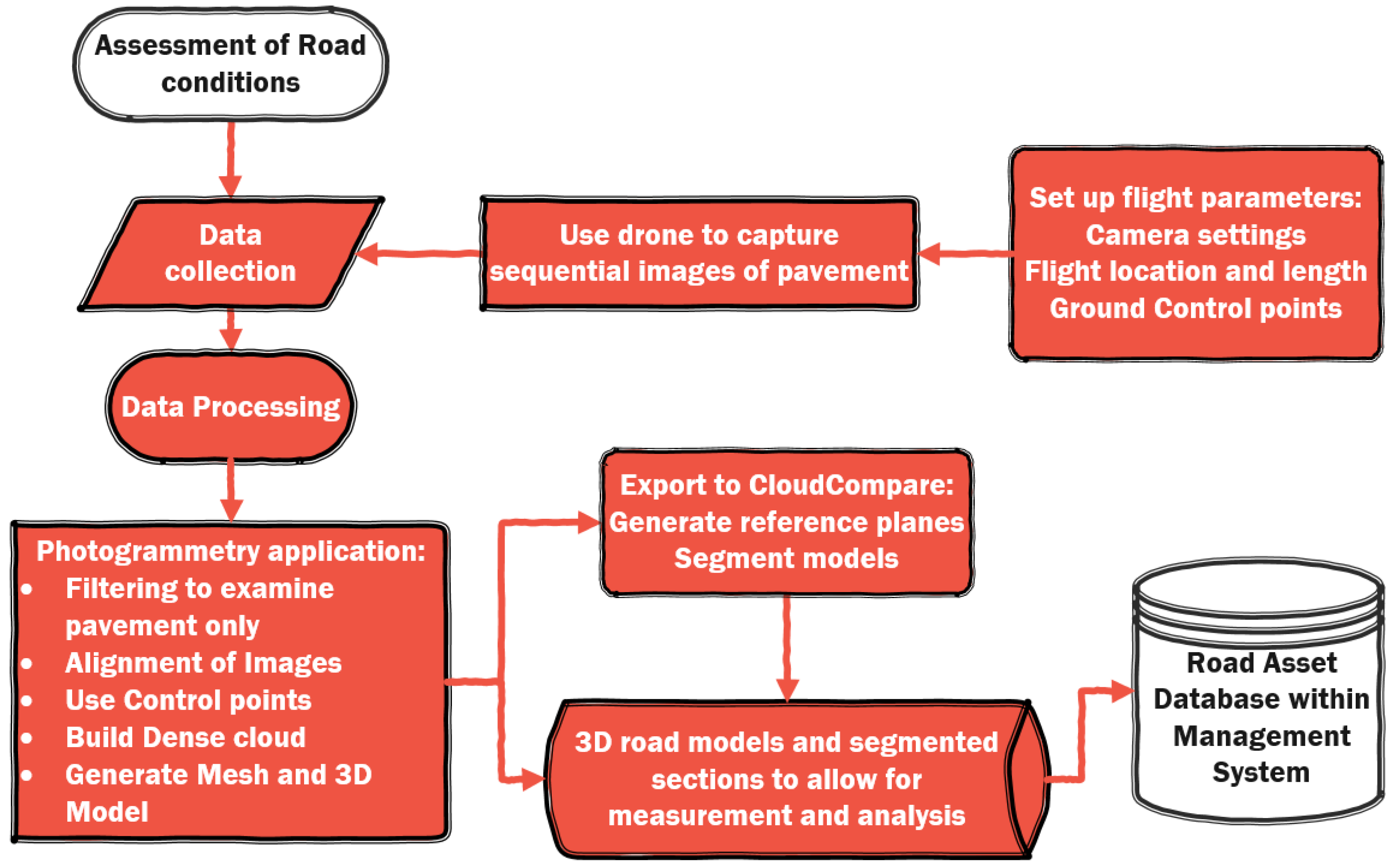
The survey roadway was straight and surrounded by trees and open greenery areas. The survey was also carried out during a time when there was minimal traffic to avoid cars blocking the view of the roadway. As mentioned previously, this is a limitation of the process and it would be difficult to survey a heavily trafficked section, as the drone would not be able to visualize the road and the distresses. The survey was also done during a period where there was minimal wind. The drone itself has a maximum wind speed resistance of 29–38 km/h so this also represents a limitation that must be considered during surveys. With heavy winds, getting stable images could be a problem and would result in poor models. The trees that are present in the section also present a challenge to the process as they will cast shadows across the road section and the colour of the resulting model will have a different colour at those points. However, for the metric evaluation, the presence of the dark points will not have an effect. For the survey, a typical SfM workflow was utilized and this is illustrated in Figure 7. The survey itself took approximately twenty minutes and GPS points on the ground taken by the road authority were used as ground control points for the metric scaling of the subsequent models. This time frame is important as it does represent a limitation of the technique as surveys over longer sections will require recharging the battery of the drone or using multiple batteries as the battery has an approximate life of thirty minutes.
During the survey of the pavements, the flight was pre-set using specific flight settings of the drone. One trip was made across the surface. Whilst multiple trips across the surface could produce more images and possibly a higher accuracy with more details, the survey is limited by the drone battery, which limits the time possible for one survey. Additionally, by using one strip, the workflow becomes more practically applicable and more easily adapted for practitioners. The use of one long burst of images across the surface could produce a deformed 3D model so care must be made to use control points along the surface. This was done using eight coordinated points in every 200 m section of the pavement, which can be considered appropriate based on previous studies [56]. The errors of these residuals are given in Section 3.
Furthermore, by controlling the camera specifications and settings, the settings would not change per image and therefore there would be consistency in the image dataset. This is important because if an automated camera setting is used for the camera, images would have different environmental effects and matching images could cause issues for the 3D replication. The images were taken in sequence moving horizontally across the pavement with the camera focusing downwards at the pavement surface allowing for an estimated overlap of 70% by an image with the GPS of the drone being utilized for location assessment. Within the settings, the drone was instructed to automatically take images every 2 s to allow the overlap of images needed for the process. The images were also captured in their RAW format to take advantage of the number of colours and complexities that can be represented in this format as opposed to the typical jpeg format which has sixteen times less colour and uses lossless compression, which allows them not to suffer from image-compression artefacts. The images captured could then be transferred to the software maximizing the colours available in the original files.
Following this, the images were transferred to the SfM software, Agisoft Metashape [57] where the SfM pipeline as depicted in Figure 7 was used to replicate 3D models of the surveyed pavement section. Within the software, there are options for calibration and compensation for the rolling stock using pre-calibrated value but these would not be applicable for such a low-level camera and survey and could result in worse results. Any self-calibration would also result in an elongated and difficult workflow that would affect the practicality of implementing it in a road authority. The use of ground control can be considered satisfactory for this type of workflow. In the process, images and corresponding point clouds were filtered to ensure that the model would only depict the pavement and not the side elements of the pavement such as the sidewalk or trees. Once the 3D models were generated, the models were transferred to the open-source software, CloudCompare [58] to examine the defects and identify the distresses existing on the pavement sections. This methodology employed to examine the defects is represented in Section 2.2.
2.2. Application of RANSAC(RANdom SAmple Consensus) Segmentation Algorithm
After the models were transferred to CloudCompare, different segmentation techniques were considered based on previous research and the appearance of the models. In earlier works, the RANSAC segmentation algorithm [59] was considered for segmenting pavement sections [28]. This algorithm functions by attempting to extract shapes from a model by grouping specific geometric features of different types of shapes based on the number of points set out by each category by the user.
The pseudocode for the algorithm is given below in Algorithm 1 [59]:
| Algorithm 1 Extracting Shapes in point Cloud P |
| 1: Ψ ← Ø {extracted shapes} |
| 2: C ← Ø {shape candidates} |
| 3: repeat |
| 4: C ← C ∪ new Candidates () |
| 5: m ← best Candidate (C) |
| 6: if P(|m|, |C|> pt then |
| 7: P ← P\Pm {remove points} |
| 8: Ψ ← Ψ ∪ m |
| 9: C ← C\Cm {remove invalid candidates} |
| 10: end if |
| 11: until P(τ, |C|> pt |
| 12: return Ψ |
Within this, the algorithm considers a point cloud P = {p1, …, pN} and outputs a primitive set of shapes Ψ = {Ψ1, …, Ψn} which have a corresponding disjoint set of points PΨ1 ⊂ P, …, P Ψn ⊂ P and also indicates the remaining points that have not been grouped and are considered removed. The algorithm is run for several iterations with the highest scoring primitive being sought after. Once the user-defined minimal shape size for the point cloud is reached the process will conclude. This is important as this size can be defined by the user and is based on the overall point cloud size. For the implementation, the H-RANSAC plugin within CloudCompare was utilized. The plugin can be used to detect and isolate particular shapes, specifically planes, spheres, cylinders, cones and tori. As the pavement surface can be thought of as a plane, the focus within this study was using this shape to define a reference plane or rather a standard road profile from which the distresses could be referenced from. Depth maps from this plane could then be used to identify the deformation levels of the pavement and to isolate the major distressed pavement sections.
2.3. Application of 2.5D Quadric Fit Algorithm
In previous works, the segmentation was done on smaller pavement sections, which have a flatter planar reference shape, but for sections over larger lengths, it is likely that there will be some slope on the road and a direct planar reference could be difficult to achieve with the first RANSAC segmentation method. To combat this, an alternative approach was also considered using a 2.5D quadric algorithm. The 2.5D quadric would be fitted onto the 3D model. This is done to find the flattest dimensions within the model but unlike a fully planar fit, the 2.5D shape more closely mimics a 3D structure and therefore would more adequately handle the road slope. As conditions are likely to change with different environments and different distresses, this approach is flexible enough to be adapted in different circumstances.
The quadric is then visualized as a triangular mesh and this allows the computation of the deviation of the plane from the actual 3D model. This deviation would therefore represent the deformations that are present in the model and correspondingly the road section forming the depth map similar to the process outlined in Section 2.2 and using that to isolate and analyse the distressed sections of the pavement. The implementation of the algorithm was again done within CloudCompare. A comparison between this methodology and the RANSAC one was subsequently done to understand the differences and identify when to apply either algorithm.
2.4. Assessment of Level of Distress
Once the models are segmented and the depth maps generated, the next step is to analyse the level of deformation present on the road. To do this, the distribution of changes in height between the generated 2.5D quadric and the actual pavement were considered. The differences are measured across the model’s surface and can be extracted as a CSV file for analysis. Using this information, Equations (3)–(5) could then be applied to give a metric on the level of distress across the pavement.
Given that the models obtained are metrically accurate enough to detect distresses and are scaled, the information can give a practitioner a quick understanding of the level of distress over different sections and thus prioritize particular sections for intervention. Following this, recommendations are made within the study using the results from different sections of the surveyed road.
3. Results and Discussions
3.1. 3D Pavement Models
The complete surveyed section was first generated before any subsections were done. In Table 3, the specifications and results of the complete pavement model are shown. Additionally, the RMSE values for the ground control and checkpoints are given in Table 4 along the three main axes. The RMSE values are adequate given the level of details required and the size of typical pavement distresses [54] and are in line with expectations of error based on the pixel size and the points used [60].
The first important result is that of the GSD, which has a value that is less than the required value, as previously identified in Section 2.1. Therefore, this allows for the appropriate metric evaluation of distresses within the model. The number of mesh faces as mentioned within the table describes the level of detail within the model and the high number is indicative of the large model that was generated given the section length. A visual inspection of the model would yield a better understanding of the details. Images showing the generated 3D model are given in Figure 8. Within the figure, the position of the drone through the survey is also shown illustrating the overlapping images captured from above the pavement’s surface.
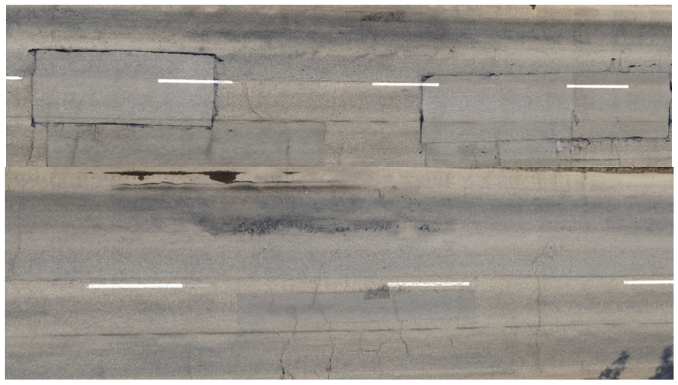
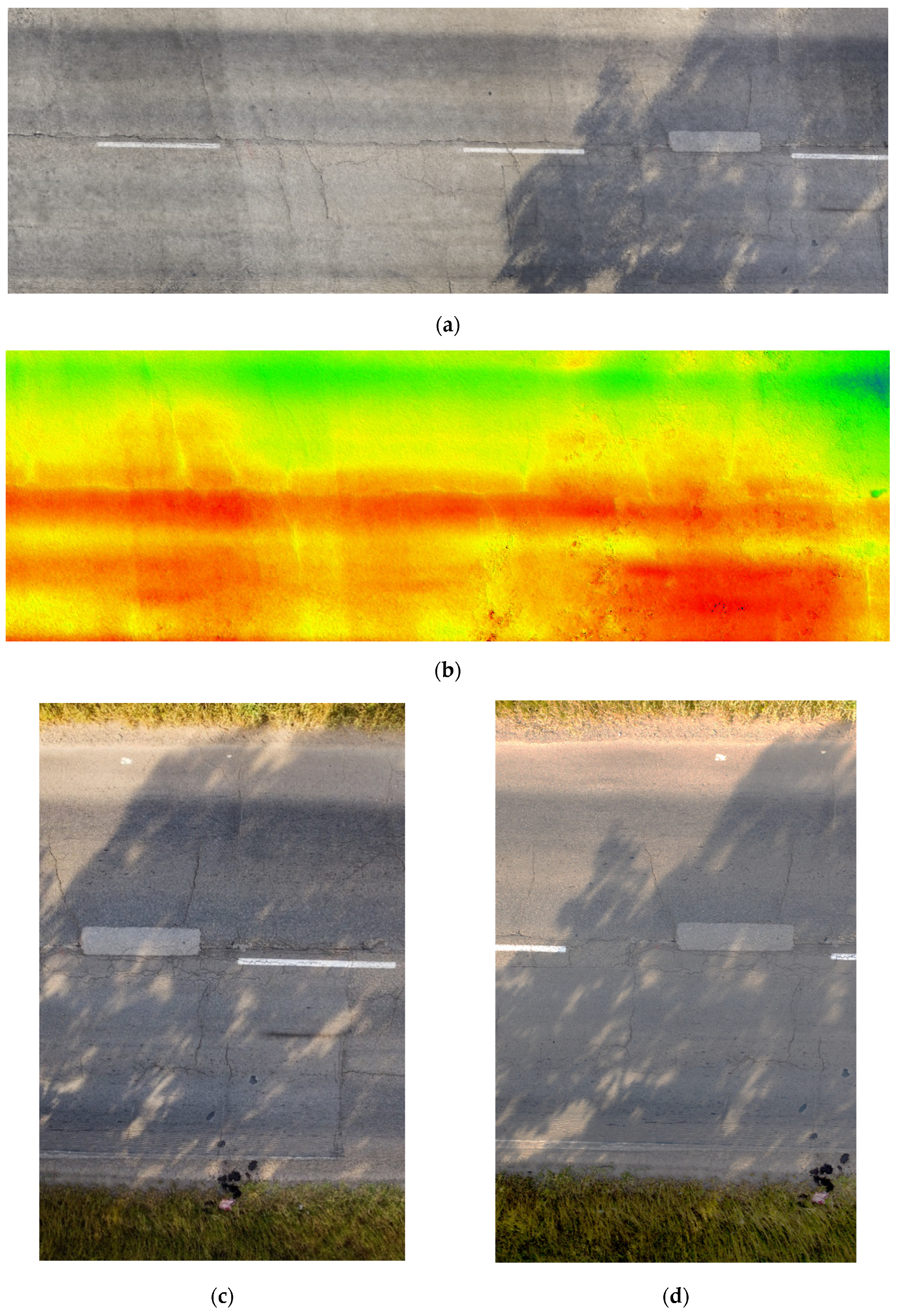
As the pavement section is quite large, to have a better understanding of the level of details, sections were cropped and these are displayed in Figure 9. Within these images, the distresses are more clearly seen which include cracking, rutting and depressions. It is also important to note that the models are scaled and therefore a metric evaluation of these particular distresses is possible. Images of the original drone imagery are also provided in Figure 10. In the original images, the grass edges are shown as well.
3.2. Application of RANSAC Segmentation
Following the generation of the 3D model of the entire pavement section, the subsequent step was the analysis of the models using the previously mentioned segmentation strategies. The first employed strategy was the utilization of the RANSAC algorithm, which allows extraction of shapes from the targeted point clouds. In this implementation, the assignment of the value for the minimum support points is needed.
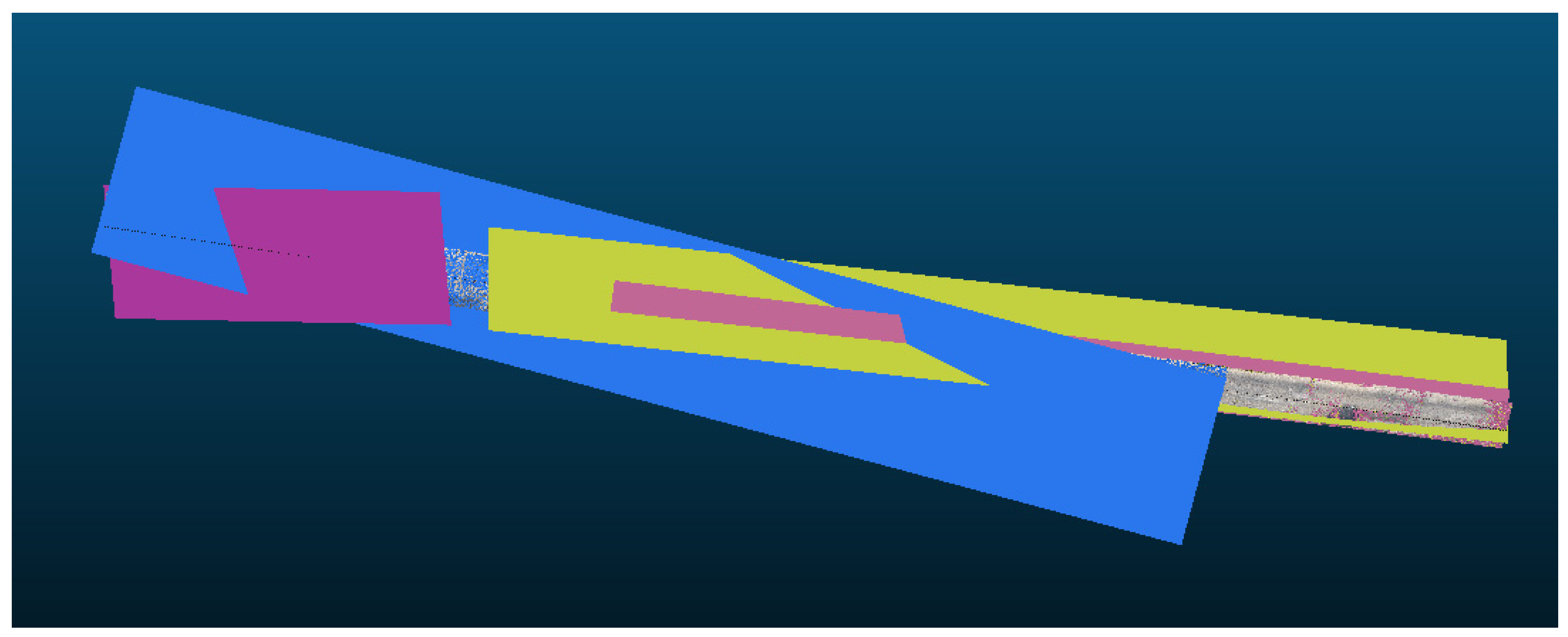
For the largest model under analysis, the total number of points in the point cloud was 90 million points. This represents a sectional area of approximately 8000 m2 of the ground surface. Using this and parameters previously used to segment pavement models using the RANSAC algorithm, a value of 50,000 points was initially assigned for splitting the object to produce the reference plane. However, when using this value too many planes were created and this is visualized in Figure 11.
Following this, trials using 70,000–120,000 points were considered. However, the slope of the road was an issue as planes were generated at inclined angles as shown in Figure 12.
Therefore, this proved to be an inappropriate methodology for the full section. However, when applied to subsections where the slope was nearly zero it was possible to generate adequate reference planes as is shown in Figure 13.
Therefore, it can be surmised that this application only works when small sections of roads are considered and therefore for a network or longer road it is not useful to apply this segmentation strategy. Given this, the consideration of the 2.5 quadric was very important.
3.3. Application of Quadric Plane and Subsequent Segmentation
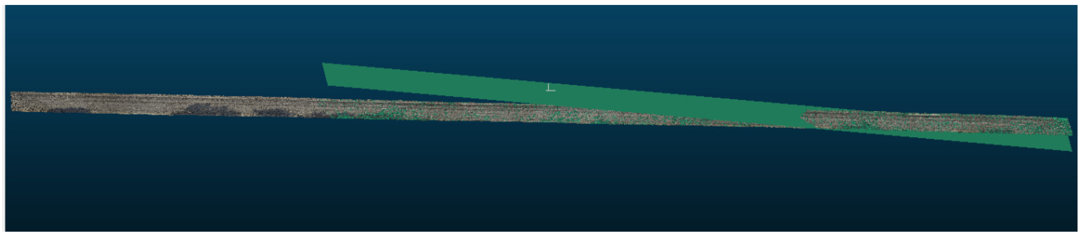
For the application of the quadric plane, the plugin was utilized within CloudCompare where the plane was generated upon the surface of the 3D model. With the quadric application, a root mean square (RMS) of 0.0084 m was achieved. The RMS value is a good indication of the closeness of the fit between the newly created reference plane and the actual model. A visualization of the plane on the model is given in Figure 14.
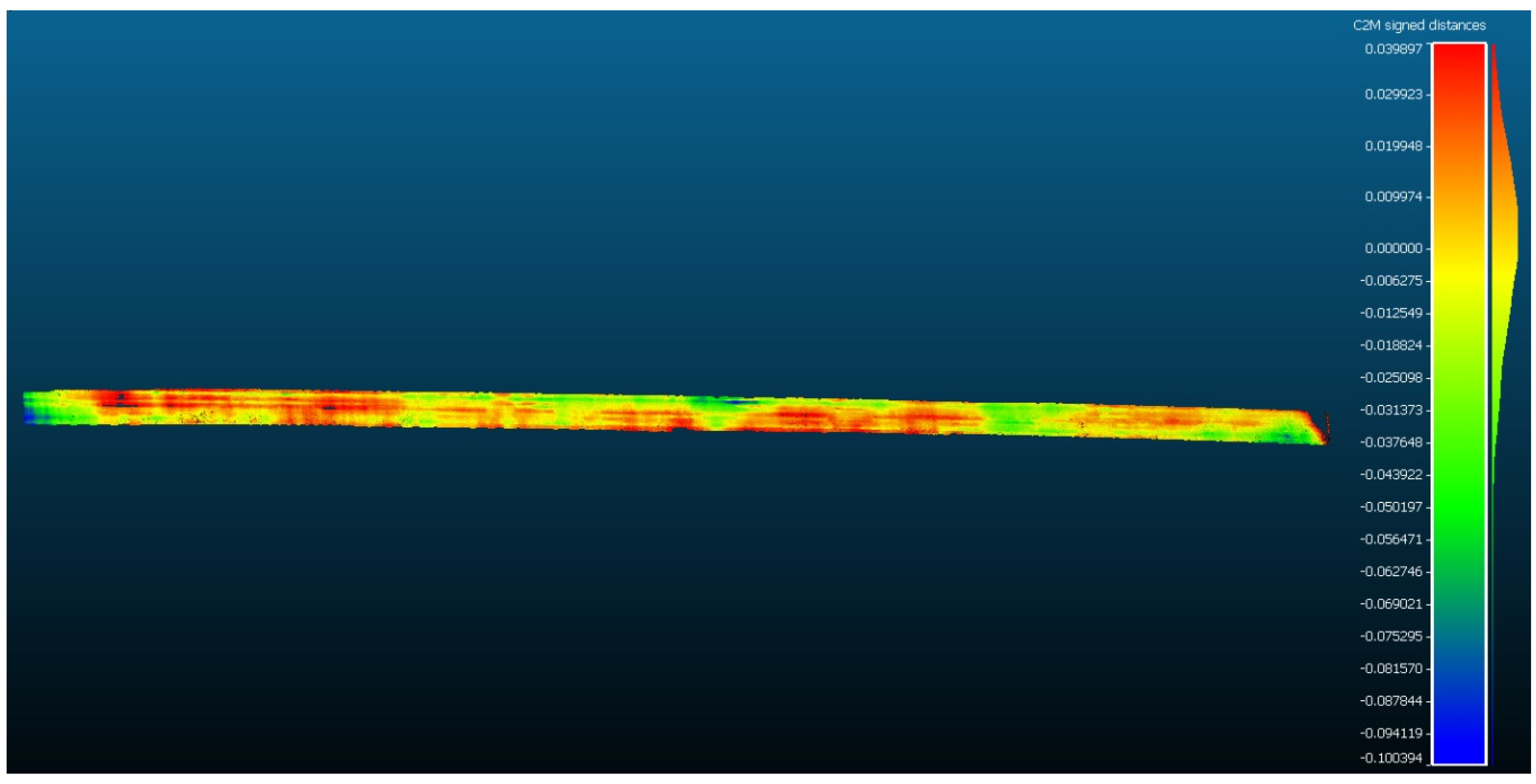
After the plane was adequately assigned to the model, a computation of the distance between the plane and the model could then be calculated using the “C2M” distance computation within CloudCompare. This can be used to establish depth maps of the road section depicting points of deformation and degradation. An overall depth map illustrating the differences between the reference plane and the model is shown in Figure 15, with the colours emphasizing distressed areas.
Using the depths measured within this overall model, further segmentation can be made at various points of analysis along the model. Examples of particular points of emphasis along the model are given in Figure 16 and Figure 17.
Within the examples, the points along the crack are visualized and can be isolated from the remainder of the model as well. Using the segmentation applications, the isolated sections will generate important metric analysis and information for road authorities. Metric assessments of any sections would be able to output area and volumetric measurements, which in turn can result in values of the volume or area of the cracks, depressions and other deformations, which are key to the evaluation of the pavement and the overall network. The metric evaluations and analysis can also be made at cross-sections along the model. An example of this is depicted in Figure 18 where the 3D model was transferred to a computer-aided design (CAD) software, Rhino 3D [61], and cross-sections implemented at 0.5 m intervals along the model. Within the section shown, rutting and surface roughness are shown and using the model, the exact metric values of deviation can be established.
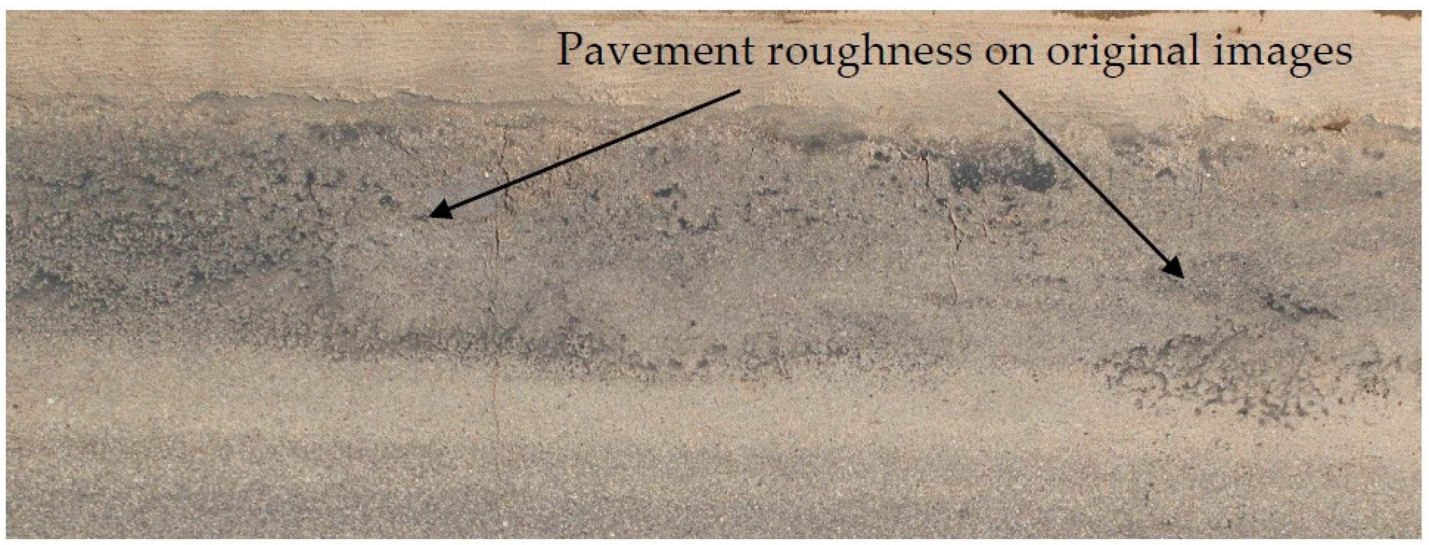
Whilst it is possible for the model itself to display roughness, a check using the original images reveals the rough sections of the pavement as shown in Figure 19 below. The pavement suffers from excessive roughness on the pavement sides where there is also rutting likely caused by traffic loading by heavier vehicles in these lanes. This is common in these types of roadways.
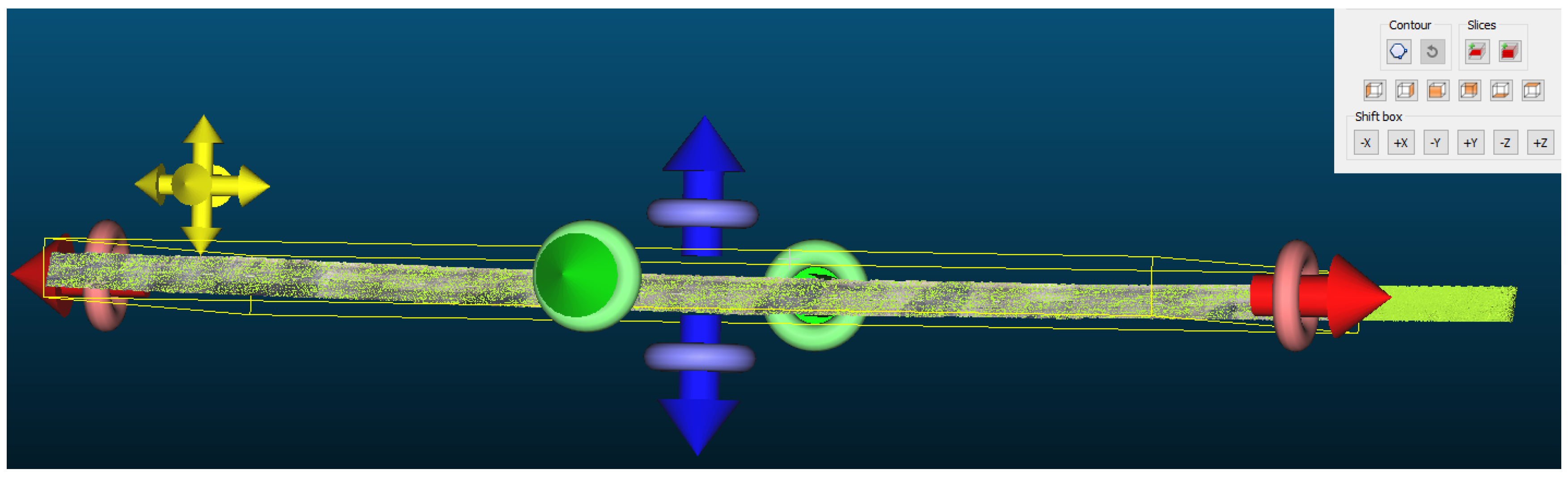
To understand the overall levels of distress at different sections, the model was then split using the cross-sectional tools available in CloudCompare as illustrated in Figure 20. Using the tools, three subsections were created and using these sections, analysis of the deformations were done to understand the average level of distress on the various sections.
3.4. Analysis of the Level of Distress over Pavement Sections
With the segmentation complete, the formulae given in Section 2.4 were used to understand the general road condition and the deformations present on the road. The results from these calculations are given in Table 5. This was done using the outputs from the CSV file expressing the deviations of the surface of the model from the established reference planes.
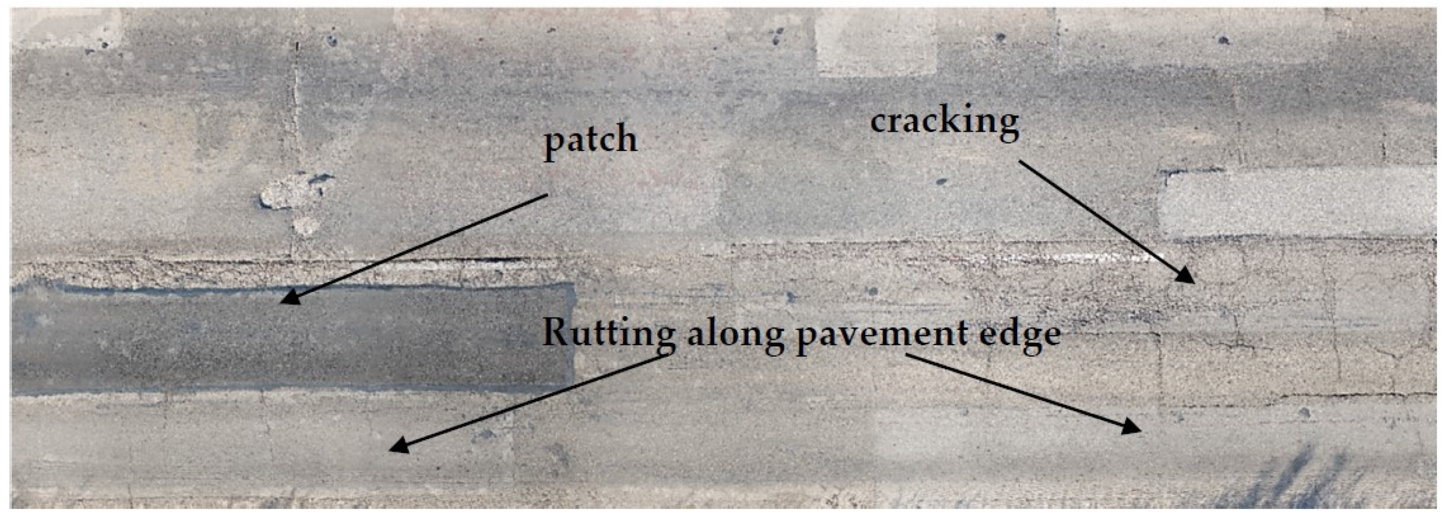
From the figures, it can be seen that the overall section has an average level of distress of 20% of its pavement surface. In the other three sub-sections considered the distress is greater with subsection 1 having the largest degree of distress of over 40% degradation. The colour coding (green to red) used in Table 5 highlights the levels of severity, with red representing the most damaged sections. From this coding, it is clear that the most damaged section is sub-section 1. A closer examination of this section reveals tremendous cracking, patched areas and highly rutted areas as shown in Figure 21.
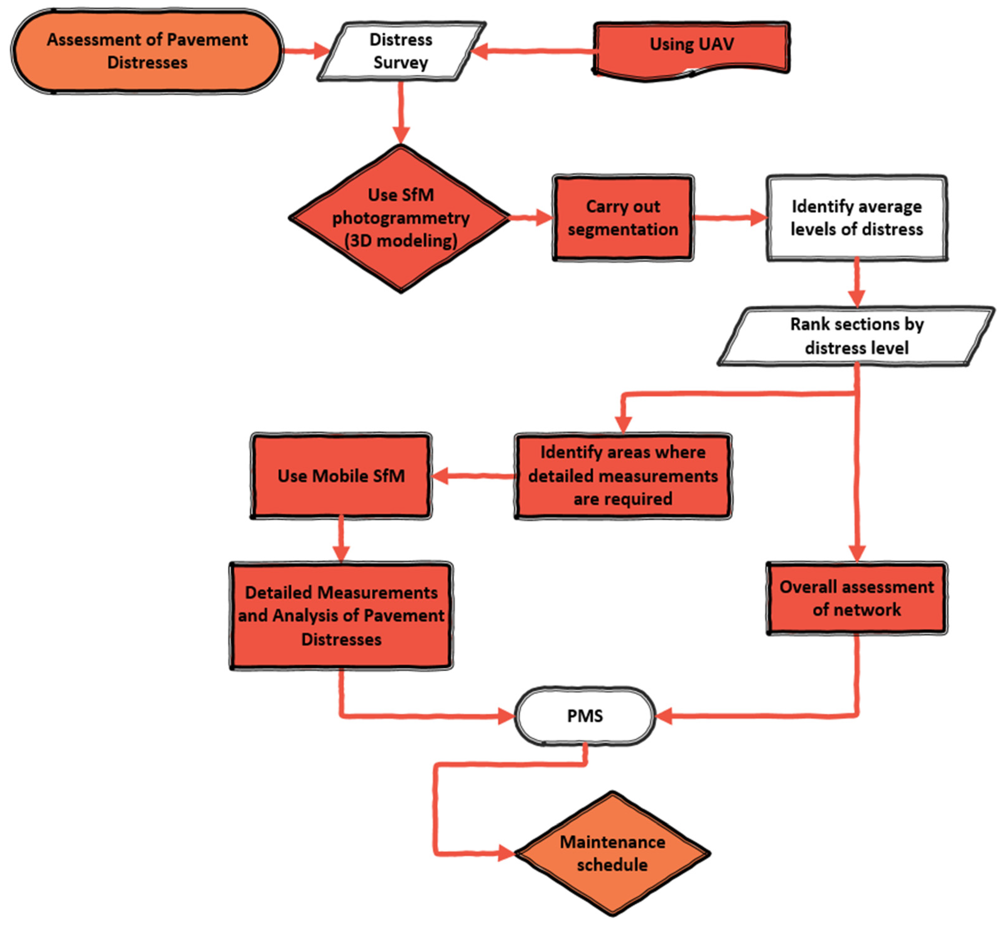
This was done to illustrate how road managers can use the information. If surveys are carried out using the same methodology for a large number of road sections, then the average level of distress can be generated per section and the managers would have a clear idea of which sections are in the poorest conditions. The list would then be kept in their database and continually updated at various time intervals to schedule and plan future road interventions. The models can also be used in a workflow within Agisoft Metashape to develop a digital elevation model (DEM) which refers to the terrain and can allow for contour mapping. High-quality orthophoto maps can also be generated from the UAV imagery [62] and kept in the road asset database. This can be made on a continual basis to monitor changes in the displacement of the pavement over time. Similar workflows have been validated in analysing road deformations due to natural disasters and hazards like landslides [63]. Within these workflows, surveys are carried out continuously over years to understand the changes in the model using the DEM and a similar approach can be used within this domain. The use of the DEM could also prove useful in determining patterns of patches but more than one comparison is needed for assertions on patterns could be readily adapted. Nevertheless, whilst there are no available comparable DEMs, at different points of time over the years, for the road under analysis, the approach in this study provides for an analysis given limited data and provides the platform for the future development of the pipeline. This situation is also one that is likely to occur in a road authority with limited resources and who need quick answers on the current state of the pavement. In a scenario where an overview is required to compute the average levels of distress as shown in Table 5, the approach in this study is sufficient. Given this, a workflow can be developed around the type of information yielded from the current process. This is illustrated in Figure 22.
Within the workflow, the techniques would be used to rank road sections within a network based on the average distress levels. This would help users to understand the overall conditions of the network. Additionally, the UAV models will highlight particular points, where additional information may be needed and at these points, similar SfM techniques can be applied using mobile imagery instead as adequately demonstrated by previous studies [28]. With the systems combined, the road authority would have vital road condition data to plan their maintenance programs.
4. Conclusions
The study carried out in this paper set out to utilize drone imagery to recreate 3D models of a road and then use the models to monitor and analyse the pavement surface conditions. Previous work validated the accuracies of using structure-from-motion techniques to generate 3D models of pavement distresses and this study was built from this pipeline. To further utilize the techniques over a pavement section and using the drone imagery, a case study was developed using a highly distressed road section to display how the models can be generated and then a workflow was built to segment the models from the UAV imagery. The focus of the study is on how the techniques can be exploited to serve as a platform for helping monitor pavements. Because of this, the most adaptable version of the techniques was considered to ensure the pipeline could be easily understood in a civil engineering application and domain.
Different segmentation strategies were considered and it was shown that for longer road sections, different segmentation techniques are needed as the road slope does not allow for an adaption of a flat plane as was done in previous studies. The segmentation techniques used in the study allowed a reference section to be developed to calculate the deformations along the road profile, which could alert practitioners to the particular points of concern on the network. An analysis pipeline was also created to generate a metric, which would display the average level of distress of a particular model or section. This was developed using a statistical analysis of the deviations present in the model when related to a reference plane developed within the study. Different sections of the model were used to show that the process would give a value that can relate to the required intervention for that section. Using this process for several different surveys over a network, a road authority would be able to have a greater understanding of the worst sections within the network and could then make appropriate intervention strategies. As was highlighted in Figure 1, the outputs of the PMS are the timeline for maintenance strategies and the type of intervention and this process yields information to characteristics the pavement conditions that would lead to the desired output of establishing appropriate maintenance timelines.
The pipeline is not only reliable but also affordable as the costliest acquisition is the drone and the cost of this piece of equipment is marginal compared to the typical techniques involving survey vehicles. It should also be stressed that the drone used is not the latest version from the company and future drones will have even better cameras and specifications, which will in turn yield even better resolutions and models. Additionally, it must be reinforced here that as the process was carried out with flexible user-friendly techniques and algorithms, the process is flexible and would not require significant resources to be practically implemented. Future work will include an analysis of a wider network to demonstrate the capacity of the process along with more metric analysis of particular points on the network and the associated distress categories at these points. Finally, based on the results and output workflow, the study helps take the automation of the detection of road conditions a step further.
Author Contributions
Conceptualization, R.R.; methodology, R.R., L.I. and G.D.M.; software, R.R. and L.I.; validation, R.R. and G.D.M.; formal analysis, R.R. and G.D.M.; investigation, R.R., L.I. and G.D.M.; resources, G.D.M. and L.I.; data curation, R.R.; writing—original draft preparation, R.R.; writing—review and editing, R.R., G.D.M. and L.I.; visualization, R.R. and G.D.M. All authors have read and agreed to the published version of the manuscript.
Funding
The research presented in this paper was carried out as part of the H2020-MSCA-ETN-2016. This project has received funding from the European Union’s H2020 Programme for research, technological development and demonstration under grant agreement number 721493.
Acknowledgments
The authors would like to thank Bernard Sidi, who assisted the researchers during the road surveys by providing ground support to capture the images during the survey.
Conflicts of Interest
The authors declare no conflict of interest.
References
- Vandam, T.J.; Harvey, J.T.; Muench, S.T.; Smith, K.D.; Snyder, M.B.; Al-Qadi, I.L.; Ozer, H.; Meijer, J.; Ram, P.V.; Roesier, J.R.; et al. Towards Sustainable Pavement Systems: A Reference Document FHWA-HIF-15-002; Federal Highway Administration: Washington, DC, USA, 2015.
- International Road Federation (IRF). IRF World Road Statistics 2018 (Data 2011–2016); International Road Federation (IRF): Brussels, Belgium, 2018. [Google Scholar]
- Peterson, D. National Cooperative Highway Research Program Synthesis of Highway Practice Pavement Management Practices. No. 135; Transportation Research Board: Washington, DC, USA, 1987; ISBN 0309044197. [Google Scholar]
- Waidelich, W. Guidance on Highway Preservation and Maintenance-Memorandum; U.S. Department of Transportation-Federal Highway Administration: Washington, DC, USA, 2016.
- Mith, K.L.; Peshkin, D.; Wolters, A.; Krstulovich, J.; Moulthrop, J.; Alvarado, C. Guidelines for the Preservation of High-Traffic-Volume Roadways; National Academies of Sciences, Engineering, and Medicine: Washington, DC, USA, 2011; ISBN 9780309128926. [Google Scholar] [CrossRef] [Green Version]
- Rouse, P.; Chiu, T. Towards optimal life cycle management in a road maintenance setting using DEA. Eur. J. Oper. Res. 2009, 196, 672–681. [Google Scholar] [CrossRef]
- Schnebele, E.; Tanyu, B.F.; Cervone, G.; Waters, N. Review of remote sensing methodologies for pavement management and assessment. Eur. Transp. Res. Rev. 2015, 7. [Google Scholar] [CrossRef] [Green Version]
- Radopoulou, S.C.; Brilakis, I. Improving Road Asset Condition Monitoring. Transp. Res. Procedia 2016, 14, 3004–3012. [Google Scholar] [CrossRef] [Green Version]
- Coenen, T.B.J.; Golroo, A. A review on automated pavement distress detection methods. Cogent Eng. 2017, 4. [Google Scholar] [CrossRef]
- Ragnoli, A.; De Blasiis, M.; Di Benedetto, A. Pavement Distress Detection Methods: A Review. Infrastructures 2018, 3, 58. [Google Scholar] [CrossRef] [Green Version]
- Pierce, L.M.; McGovern, G.; Zimmerman, K.A. Practical Guide for Quality Management of Pavement Condition Data Collection; U.S. Department of Transportation: Washington, DC, USA, 2013.
- Paterson, W.D.O.; Scullion, T. Information Systems for Road Management: Draft Guidelines on System Design and Data Issues; The National Academies of Sciences, Engineering, and Medicine: Washington, DC, USA, 1990. [Google Scholar]
- Wang, K.C.P.; Gong, W. Automated pavement distress survey: A review and a new direction. In Proceedings of the Pavement Evaluation Conference, Roanoke, VA, USA, 21–25 October 2002; pp. 21–25. [Google Scholar]
- Arhin, S.A.; Williams, L.N.; Ribbiso, A.; Anderson, M.F. Predicting Pavement Condition Index Using International Roughness Index in a Dense Urban Area. J. Civ. Eng. Res. 2015, 5, 10–17. [Google Scholar] [CrossRef]
- Laurent, J.; Hébert, J.F.; Lefebvre, D.; Savard, Y. Using 3D Laser Profiling Sensors for the Automated Measurement of Road Surface Conditions. In Proceedings of the 7th RILEM International Conference on Cracking in Pavements, Delft, The Netherlands, 20–22 June 2012; Scarpas, A., Kringos, N., Al-Qadi, I.A.L., Eds.; Springer: Dordrecht, The Netherlands, 2012; pp. 157–167. [Google Scholar] [CrossRef]
- Landa, J.; Prochazka, D. Automatic Road Inventory Using LiDAR. Procedia Econ. Financ. 2014, 12, 363–370. [Google Scholar] [CrossRef] [Green Version]
- Sairam, N.; Nagarajan, S.; Ornitz, S. Development of Mobile Mapping System for 3D Road Asset Inventory. Sensors 2016, 16, 367. [Google Scholar] [CrossRef] [Green Version]
- Luis, G.; Antunes, C. Road Rutting Measurement Using Mobile LiDAR Systems Point Cloud. ISPRS Int. J. Geo-Inf. 2019, 8, 404. [Google Scholar] [CrossRef] [Green Version]
- Wix, R.; Leschinski, R. Cracking—A Tale of Four Systems. In Proceedings of the 25th Australian Road Research Board Conference, Perth, Australia, 23–26 September 2012; pp. 1–20. [Google Scholar]
- Oliveira, H.; Correia, P.L. Automatic Road Crack Detection and Characterization. IEEE Trans. Intell. Transp. Syst. 2013, 14, 155–168. [Google Scholar] [CrossRef]
- Puan, O.C.; Mustaffar, M.; Ling, T.-C. Automated Pavement Imaging Program (APIP) for Pavement Cracks Classification and Quantification. Malays. J. Civ. Eng. 2007, 19, 1–16. [Google Scholar]
- Chambon, S.; Moliard, J.M. Automatic road pavement assessment with image processing: Review and Comparison. Int. J. Geophys. 2011, 2011. [Google Scholar] [CrossRef] [Green Version]
- Zakeri, H.; Nejad, F.M.; Fahimifar, A. Image Based Techniques for Crack Detection, Classification and Quantification in Asphalt Pavement: A Review. Arch. Comput. Methods Eng. 2017, 24, 935–977. [Google Scholar] [CrossRef]
- Majidifard, H.; Jin, P.; Adu-Gyamfi, Y.; Buttlar, W.G. Pavement Image Datasets: A New Benchmark Dataset to Classify and Densify Pavement Distresses. Transp. Res. Rec. J. Transp. Res. Board 2020, 2674, 328–339. [Google Scholar] [CrossRef] [Green Version]
- Gopalakrishnan, K. Deep Learning in Data-Driven Pavement Image Analysis and Automated Distress Detection: A Review. Data 2018, 3, 28. [Google Scholar] [CrossRef] [Green Version]
- Gopalakrishnan, K.; Khaitan, S.K.; Choudhary, A.; Agrawal, A. Deep Convolutional Neural Networks with transfer learning for computer vision-based data-driven pavement distress detection. Constr. Build. Mater. 2017, 157. [Google Scholar] [CrossRef]
- Inzerillo, L.; Di Mino, G.; Roberts, R. Image-based 3D reconstruction using traditional and UAV datasets for analysis of road pavement distress. Autom. Constr. 2018, 96, 457–469. [Google Scholar] [CrossRef]
- Roberts, R.; Inzerillo, L.; Mino, G. Di Exploiting Low-Cost 3D Imagery for the Purposes of Detecting and Analyzing Pavement Distresses. Infrastructures 2020, 5, 6. [Google Scholar] [CrossRef] [Green Version]
- Roberts, R.; Inzerillo, L.; Di Mino, G. Developing a framework for using Structure-from-Motion techniques for Road Distress applications. Eur. Transp. Transp. Eur. 2020, 77, 1–11. [Google Scholar]
- Westoby, M.J.; Brasington, J.; Glasser, N.F.; Hambrey, M.J.; Reynolds, J.M. “Structure-from-Motion” photogrammetry: A low-cost, effective tool for geoscience applications. Geomorphology 2012. [Google Scholar] [CrossRef] [Green Version]
- Verhoeven, G. Taking computer vision aloft -archaeological three-dimensional reconstructions from aerial photographs with photoscan. Archaeol. Prospect. 2011, 18, 67–73. [Google Scholar] [CrossRef]
- Allegra, D.; Gallo, G.; Inzerillo, L.; Lombardo, M.; Milotta, F.L.M.; Santagati, C.; Stanco, F. Low Cost Handheld 3D Scanning for Architectural Elements Acquisition. In Proceedings of the STAG: Smart Tools and Applications in Graphics 2016, Genova, Italy, 3–4 October 2016. [Google Scholar] [CrossRef]
- Aicardi, I.; Chiabrando, F.; Maria Lingua, A.; Noardo, F. Recent trends in cultural heritage 3D survey: The photogrammetric computer vision approach. J. Cult. Herit. 2018. [Google Scholar] [CrossRef]
- Wang, K.C.P. Elements of automated survey of pavements and a 3D methodology. J. Mod. Transp. 2011, 19, 51–57. [Google Scholar] [CrossRef] [Green Version]
- Martínez, S.; Ortiz, J.; Gil, M.L. Geometric documentation of historical pavements using automated digital photogrammetry and high-density reconstruction algorithms. J. Archaeol. Sci. 2015, 53, 1–11. [Google Scholar] [CrossRef]
- Ahmed, M.; Haas, C.T.; Haas, R. Toward low-cost 3D automatic pavement distress surveying: The Close Range Photogrammetry Approach. Can. J. Civ. Eng. 2011, 38, 1301–1313. [Google Scholar] [CrossRef]
- Giordan, D.; Manconi, A.; Remondino, F.; Nex, F. Use of unmanned aerial vehicles in monitoring application and management of natural hazards. Geomat. Nat. Hazards Risk 2017, 8, 1–4. [Google Scholar] [CrossRef]
- Salvo, G.; Caruso, L.; Scordo, A. Urban Traffic Analysis through an UAV. Procedia-Soc. Behav. Sci. 2014, 111, 1083–1091. [Google Scholar] [CrossRef] [Green Version]
- Pan, Y.; Zhang, X.; Cervone, G.; Yang, L. Detection of Asphalt Pavement Potholes and Cracks Based on the Unmanned Aerial Vehicle Multispectral Imagery. IEEE J. Sel. Top. Appl. Earth Obs. Remote Sens. 2018, 11, 3701–3712. [Google Scholar] [CrossRef]
- Kang, D.; Cha, Y.J. Autonomous UAVs for Structural Health Monitoring Using Deep Learning and an Ultrasonic Beacon System with Geo-Tagging. Comput. Civ. Infrastruct. Eng. 2018, 33, 885–902. [Google Scholar] [CrossRef]
- Zhang, C. An UAV-based photogrammetric mapping system for road condition assessment. Int. Arch. Photogramm. Remote Sens. Spat. Inf. Sci. 2008, 37, 627–632. [Google Scholar]
- Zeybek, M.; Serkan, B. Road Distress Measurements Using UAV. Turk. J. Remote Sens. GIS 2020, 1, 13–23. [Google Scholar]
- Chacra, D.B.A.; Zelek, J.S. Fully Automated Road Defect Detection Using Street View Images. In Proceedings of the 2017 14th Conference on Computer and Robot Vision (CRV), Edmonton, AB, Canada, 16–19 May 2017; pp. 353–360. [Google Scholar] [CrossRef]
- Saad, A.M.; Tahar, K.N. Identification of rut and pothole by using multirotor unmanned aerial vehicle (UAV). Meas. J. Int. Meas. Confed. 2019, 137, 647–654. [Google Scholar] [CrossRef]
- Inzerillo, L.; Roberts, R. 3D Image Based Modelling Using Google Earth Imagery for 3D Landscape Modelling. Adv. Intell. Syst. Comput. 2019, 919, 627–634. [Google Scholar] [CrossRef]
- Zhang, D.; Zou, Q.; Lin, H.; Xu, X.; He, L.; Gui, R.; Li, Q. Automatic pavement defect detection using 3D laser profiling technology. Autom. Constr. 2018, 96. [Google Scholar] [CrossRef]
- Gui, R.; Xu, X.; Zhang, D.; Lin, H.; Pu, F.; He, L.; Cao, M. A component decomposition model for 3D laser scanning pavement data based on high-pass filtering and sparse analysis. Sensors 2018, 18, 2294. [Google Scholar] [CrossRef] [Green Version]
- Li, B.; Wang, K.C.P.; Zhang, A.; Fei, Y. Automatic Segmentation and Enhancement of Pavement Cracks Based on 3D Pavement Images. J. Adv. Transp. 2019, 2019, 1–9. [Google Scholar] [CrossRef]
- Akagic, A.; Buza, E.; Omanovic, S.; Karabegovic, A. Pavement crack detection using Otsu thresholding for image segmentation. In Proceedings of the 2018 41st International Convention on Information and Communication Technology, Electronics and Microelectronics, MIPRO 2018-Proceedings, Croatian Society MIPRO, Opatija, Croatia, 21–25 May 2018; pp. 1092–1097. [Google Scholar] [CrossRef]
- Tan, Y.; Li, Y. UAV Photogrammetry-Based 3D Road Distress Detection. ISPRS Int. J. Geo-Inf. 2019, 8, 409. [Google Scholar] [CrossRef] [Green Version]
- Li, M.; Nan, L.; Smith, N.; Wonka, P. Reconstructing building mass models from UAV images. Comput. Graph. 2016, 54, 84–93. [Google Scholar] [CrossRef] [Green Version]
- Remondino, F.; Nocerino, E.; Toschi, I.; Menna, F. A Critical Review of Automated Photogrammetric Processing of Large Datasets. ISPRS-Int. Arch. Photogramm. Remote Sens. Spat. Inf. Sci. 2017, XLII-2/W5, 591–599. [Google Scholar] [CrossRef] [Green Version]
- Höhle, J. Oblique Aerial Images and Their Use in Cultural Heritage Documentation. ISPRS-Int. Arch. Photogramm. Remote Sens. Spat. Inf. Sci. 2013, XL-5/W2, 349–354. [Google Scholar] [CrossRef] [Green Version]
- Zhang, S.; Lippitt, C.D.; Bogus, S.M.; Neville, P.R.H. Characterizing pavement surface distress conditions with hyper-spatial resolution natural color aerial photography. Remote Sens. 2016, 8, 392. [Google Scholar] [CrossRef] [Green Version]
- Loprencipe, G.; Pantuso, A. A Specified Procedure for Distress Identification and Assessment for Urban Road Surfaces Based on PCI. Coatings 2017, 7, 65. [Google Scholar] [CrossRef] [Green Version]
- Oniga, E.; Breaban, A.; Statescu, F. Determining the optimum number of ground control points for obtaining high precision results based on UAS images. Proceedings 2018, 2, 352. [Google Scholar] [CrossRef] [Green Version]
- Agisoft LLC Agisoft Metashape Professional 2019. Available online: https://www.agisoft.com/ (accessed on 12 July 2020).
- EDF R&D/TELECOM ParisTech (ENST-TSI) CloudCompare 2016. Available online: https://www.danielgm.net/cc/ (accessed on 12 August 2020).
- Schnabel, R.; Wahl, R.; Klein, R. Efficient RANSAC for point-cloud shape detection. Comput. Graph. Forum 2007, 26, 214–226. [Google Scholar] [CrossRef]
- Carballido, J.; Perez-Ruiz, M.; Emmi, L.; Agüera, J. Comparison of positional accuracy between rtk and rtx gnss based on the autonomous agricultural vehicles under field conditions. Appl. Eng. Agric. 2014, 30, 361–366. [Google Scholar] [CrossRef] [Green Version]
- Robert McNeel & Associates Rhino3D 2018. Available online: https://www.rhino3d.com/ (accessed on 10 August 2020).
- Liu, Y.; Zheng, X.; Ai, G.; Zhang, Y.; Zuo, Y. Generating a High-Precision True Digital Orthophoto Map Based on UAV Images. ISPRS Int. J. Geo-Inf. 2018, 7, 333. [Google Scholar] [CrossRef] [Green Version]
- Cardenal, J.; Fernández, T.; Pérez-García, J.L.; Gómez-López, J.M. Measurement of road surface deformation using images captured from UAVs. Remote Sens. 2019, 11, 1507. [Google Scholar] [CrossRef] [Green Version]
Figure 1.
How pavement data is used within the pavement management system (PMS).

Figure 2.
Example of a photographic dataset obtained during a survey of a pavement section.

Figure 3.
Workflow to utilize segmentation of 3D models.

Figure 4.
Visual representation of the ground sampling distance (GSD).

Figure 5.
DJI Mavic Pro 2 drone used for surveys.

Figure 6.
Aerial overview of the roadway used for the study.

Figure 7.
SfM pipeline utilized for generating pavement models.

Figure 8.
Full model produced by drone imagery. (a) First section of model (b) Second section of model.
Figure 8.
Full model produced by drone imagery. (a) First section of model (b) Second section of model.

Figure 9.
Cropped sections of the pavement model’s surface ((top) image shows a cracked and rutted sub-section and the (bottom) image shows a sub-section with depression, cracking and rutting distresses).
Figure 9.
Cropped sections of the pavement model’s surface ((top) image shows a cracked and rutted sub-section and the (bottom) image shows a sub-section with depression, cracking and rutting distresses).

Figure 10.
Examples of the original drone imagery used for the models. (a) First example of original imagery from section (b) Second example of original imagery from section.
Figure 10.
Examples of the original drone imagery used for the models. (a) First example of original imagery from section (b) Second example of original imagery from section.

Figure 11.
Visualization of RANSAC algorithm using inadequate minimum number of support points.

Figure 12.
Errors in using RANSAC application.

Figure 13.
Application of plane shape through RANSAC algorithm.

Figure 14.
Application of quadric plane to model.

Figure 15.
Application of quadric algorithm to the pavement section.

Figure 16.
Top—first example of a segmented pavement section, bottom—original drone images from the section. (a) 3D model of pavement section; (b) Segmented 3D model (c) First example of original imagery from section; (d) Second example of original imagery from section.
Figure 16.
Top—first example of a segmented pavement section, bottom—original drone images from the section. (a) 3D model of pavement section; (b) Segmented 3D model (c) First example of original imagery from section; (d) Second example of original imagery from section.

Figure 17.
Top—second example of a segmented pavement section, bottom—examples of the original drone images. (a) 3D model of pavement section; (b) Segmented 3D model; (c) First example of original imagery from section; (d) Second example of original imagery from section.
Figure 17.
Top—second example of a segmented pavement section, bottom—examples of the original drone images. (a) 3D model of pavement section; (b) Segmented 3D model; (c) First example of original imagery from section; (d) Second example of original imagery from section.

Figure 18.
Cross-sections drawn on model with computer-aided design (CAD) at a prescribed distance.

Figure 19.
Original drone image highlighting pavement roughness.

Figure 20.
Generating cross-sections of model.

Figure 21.
Cropped section from subsection 1.

Figure 22.
Workflow to utilize SfM techniques and information in PMS.


Table 1.
Devices used for detecting pavement distresses.
| Type of Detection | Device |
|---|---|
| Image-based Cameras | CCD (charge-coupled device), infrared, CMOS (metal-oxide-semiconductor sensor), line-scan, video, black-box, smart phone, retro reflectivity meter |
| Accelerometer | The device on: a smartphone, the wheel, the wheel axis, in-car |
| 3D Sensors | Laser profiler, line projection, stereovision, Kinect device, ground penetrating radar, structured light, photometric stereo |
| Microphone | A device placed: on a tyre, near the road, beneath the car |
| Sound propagation | Sonar device |
| Pressure | Pressure sensor |
| Friction | Tyre traction, angled wheel |
| Deflectometer | Falling weight deflectometer (FWD), dynamic rolling weight deflectometer (RWD) |
Table 2.
Specifications of the camera on the UAV used for structure-from-motion (SfM) surveys.
| Device | DJI Mavic 2 Pro |
|---|---|
| Drone weight (grams) | 907 |
| Camera resolution (megapixel) | 20 |
| Image Size (pixel) | 5568 × 3648 |
| Sensor size (mm) | 13.2 × 8.8 |
| Focal length (35 mm eq.) | 28 |
| ISO Sensitivity | 100 |
| Exposure time | 0.001 (shutter speed of 1/1000) |
| Aperture | f/2.8 |
Table 3.
Survey specifications for full section.
| Device | DJI Mavic 2 Pro |
|---|---|
| Distance from the pavement (m) | ~8 |
| Number of photos taken (-) | 554 |
| Ground sample distance (GSD) (mm/pixel) | 0.97 |
| Number of points created in SfM software (-) | 90,508,878 |
Table 4.
Control and checkpoints’ RMSE values.
| Direction | Control Points RMSE (m) | Checkpoints RMSE (m) |
|---|---|---|
| X error | 0.0078 | 0.0095 |
| Y error | 0.0082 | 0.0112 |
| Z error | 0.0079 | 0.0119 |
Table 5.
Distress results of pavement models.
| Measurement | Full Section | Subsection 1 | Subsection 2 | Subsection 3 |
|---|---|---|---|---|
| Length of section (m) | 1000 | 200 | 250 | 300 |
| Average height of deformation (m) | 0.020 | 0.043 | 0.032 | 0.025 |
| Volume of distressed pavement surface (m3) | 160.80 | 69.02 | 64.50 | 50.20 |
| Average level of distress over section (%) | 20.35 | 43.14 | 32.25 | 25.10 |
Publisher’s Note: MDPI stays neutral with regard to jurisdictional claims in published maps and institutional affiliations. |
© 2020 by the authors. Licensee MDPI, Basel, Switzerland. This article is an open access article distributed under the terms and conditions of the Creative Commons Attribution (CC BY) license (http://creativecommons.org/licenses/by/4.0/).
Share and Cite
MDPI and ACS Style
Roberts, R.; Inzerillo, L.; Di Mino, G. Using UAV Based 3D Modelling to Provide Smart Monitoring of Road Pavement Conditions. Information 2020, 11, 568. https://0-doi-org.brum.beds.ac.uk/10.3390/info11120568
AMA Style
Roberts R, Inzerillo L, Di Mino G. Using UAV Based 3D Modelling to Provide Smart Monitoring of Road Pavement Conditions. Information. 2020; 11(12):568. https://0-doi-org.brum.beds.ac.uk/10.3390/info11120568
Chicago/Turabian StyleRoberts, Ronald, Laura Inzerillo, and Gaetano Di Mino. 2020. "Using UAV Based 3D Modelling to Provide Smart Monitoring of Road Pavement Conditions" Information 11, no. 12: 568. https://0-doi-org.brum.beds.ac.uk/10.3390/info11120568
Note that from the first issue of 2016, this journal uses article numbers instead of page numbers. See further details here.