A Model for the Frequency Distribution of Multi-Scale Phenomena


1
Istituto di Informatica e Telematica (IIT–CNR), Via G. Moruzzi 1, 56124 Pisa, Italy
2
Dipartimento di Matematica, University of Parma, Parco Area delle Scienze 53/A, 43124 Parma, Italy
3
Dipartimento di Informatica, University of Pisa, Largo Pontecorvo 3, 56127 Pisa, Italy
*
Author to whom correspondence should be addressed.
Information 2020, 11(12), 580; https://0-doi-org.brum.beds.ac.uk/10.3390/info11120580
Submission received: 17 November 2020
/
Revised: 9 December 2020
/
Accepted: 11 December 2020
/
Published: 13 December 2020
Abstract
:Frequency analysis is often used to investigate the structure of systems representing multi-scale real-world phenomena. In many different environments, functional relationships characterized by a power law have been recognized, but, in many cases this simple model has turned out to be absolutely inadequate and other models have been proposed. In this paper, we propose a general abstract model which constitutes a unifying framework, including many models found in literature, like the mixed model, the exponential cut-off and the log-normal. It is based on a discrete-time stochastic process, which leads to a recurrence relation describing the temporal evolution of the system. The steady state solution of the system highlights the probability distribution, which underlies the frequency behavior. A particular instance of the general model, called cubic-cut-off, was analyzed and tested in a number of experiments, producing good answers in difficult cases, even in the presence of peculiar behaviors.
1. Introduction
A common activity in statistical science is the collection and the investigation of data in which underlying phenomenon can be described by random variables. Sometimes, data, for example human heights, are normally distributed. However, there exist many phenomena, called scale-free, where the data cannot be classified as normal distributions because the values do not gather around a mean value but span many orders of magnitude. Occurring in a wide variety of physical, biological, social, and information environments, these phenomena are assumed to have some common similarity in the structure of the underlying probability mechanisms [1].
To describe relations and processes occurring in real-world phenomena, different structures can be employed. A scalar phenomenon is characterized by a single distribution of values, called degrees, associated to given items. Examples of these phenomena are the world wealth or the word frequency in natural languages or the large cities populations.
A more complex structure is represented by the graphs (see Reference [2] and its extensive bibliography), where the edges provide connections among the nodes. The items are the nodes, and the number of edges connected to a node is its degree. A classical example is the graph which describes the structure of the web, where the nodes and the edges represent, respectively, the web pages and the links from one page to another. Graphs like this apply to many man-made and naturally occurring phenomena.
One of the most used methods to investigate these structures is the frequency analysis, which explores the relationship between the number of items having the same degree and the degree itself. For example, the analysis of large subsets of the web has shown that there are many pages with a small degree and few pages with a large degree.
Some phenomena belonging to different environments, e.g., the distribution of wealth in a society or the frequencies of words in natural languages or the frequency of the inlinks of a network, have been recognized to approximately follow functional relationships characterized by a power law [3], that is, a relation of the form , where and a is a constant scaling factor. A power law has a well-defined mean over only if and is the only scale-free distribution.
For many other phenomena, such as, for example, the frequency of the outlinks of a network [4] or the population of cities, the pure power law is absolutely inadequate. In many cases, substantial modifications are required. Among them, the following ones have often been suggested: (1) the exponential cut-off, where the power law is corrected by an exponential term responsible of a faster decay of the solution for large j, and (2) the log-normal, where a log term is responsible for a bending down for small j.
Various underlying probability distributions have been proposed for modeling the frequency behavior. They are mainly based on an attachment strategy defining the relationship between the degree of an item and the probability that its degree is increased by 1. The simplest model, which adopts a uniform attachment strategy as suggested in Reference [2], would generate a random dataset with most items having a comparable number of degrees. This behavior does not reflect the real-world datasets, where there are many items with a very small degree and a not negligible part of hub items with high degree. To obviate this situation, a preferential attachment strategy has been proposed (see Reference [5]). This strategy complies especially with the “rich get richer” effect. A mixed model combines the uniform and preferential approaches (see, for example, Reference [6,7,8]).
To describe the frequency behavior of multi-scale phenomena, in this paper, we propose a general model, which constitutes a unifying abstract framework able to include many models found in literature, like the mixed model, the log-normal model, and the exponential cut-off model. It is based on a discrete-time stochastic process, which leads to a recurrence relation describing the temporal evolution of the system. The steady state solution of the system highlights the probability distribution, which underlies the frequency behavior and rules the strategy on which the attachment policy relies.
A particular instance of the general model, which we call the cubic-cut-off model, is taken into consideration with the aim of dealing, at the same time, with items having a very small degree or a very large degree, providing a correct characterization of the degree distributions on the full range of the available data, even in presence of peculiar behaviors. This cubic-cut-off model lends itself to a definition of the attachment strategy, which characterizes, in a simple way, the behavior of the system. It has been tested in a number of experiments, producing better answers than the classical models, even in difficult cases.
The paper is structured as follows. The structure of the datasets taken into consideration in our analysis and the formal definition of a general model from which stems our proposed cubic-cut-off model are described in Section 2.1 and Section 2.2. The discrete time stochastic process and the steady-state solution are described in Section 2.3. The classical Beta, power law, log-normal, and cut-off models are derived in Section 2.4 and Section 2.5. In Section 3, we examine the problems caused by the collection, the representation, and the fitting of the real-world data. Finally, in Section 4, we test our model in comparison with the classical ones on a collection of 39 files of data, extracted from 21 datasets, including typical examples, such as the web, the movie actors graph, the supermarket purchases, or the number of social media followers.
2. The Frequency Distribution Model
The world wealth, the word frequency in natural languages, or the large cities populations represent real-world phenomena in which structure is characterized by a single distribution of values. In order to describe the processes which guide their evolution, models of their frequency distributions are often devised. First of all, we give some definitions about the structure of the datasets we are considering.
2.1. The Structure of Datasets
The simplest way to treat real-world phenomena is to associate to each considered item, let’s say the kth one, a value which somewhat measures the feature of interest. For example, could be the number of occurrences of the kth word in a linguistic corpus or the number of inhabitants of the kth city. We say that is the degree of the kth item. The number of items having the same degree j is the frequency and is given by
An analogous function can be referred to also when we deal with phenomena described by more complex structures. We examine for example the structure implementing graphs, which are usually addressed to design models using vertices (the nodes) and edges (the links) for the interconnections. The degree of a node v is the number of links connected to v, and the number of nodes having the same degree j is given by
Definition (2) coincides with (1) if we assimilate node v to item k and to .
Generally, the values which describe real-world phenomena span many orders of magnitude. For this reason, it is common in the literature to switch to the log-log plane for their graphical representation.
2.2. The Model
We give now the definition of a general model for describing the frequency behavior of multi-scale phenomena. Such a definition, based on infinite sequences verifying simple mathematical properties, aims at setting a unifying abstract framework for many approaches found in literature.
Definition 1.
A model is a pair of positive real infinite sequences
where the sequence , with , satisfies , and the sequence satisfies
From (4), it follows that
Thanks to these relations, a model can be defined through any positive real infinite sequence such that converges to a limit , by setting
Note that, in the rest of the paper, we use the notation , with implicitly varying index j, to denote either the jth element of sequence or the whole sequence, depending on the context.
In the following section, we briefly outline the discrete-time stochastic process which leads to a model of form (3), where the sequence is the expected value of the sequence .
2.3. The Discrete-Time Stochastic Process
The frequency analysis, often used to investigate the structure of a system, allows a deep insight in the design underlying a dataset. The frequency distribution model we consider in this paper is based on the following discrete-time stochastic process: we assume that, at time t, a set of items exists, with , and that t is updated corresponding to a unit increase of the degree of an item.
Let denote the number of items having degree . Then, and . In our setting and are random variables, in which expected values are and , respectively.
Let denote the probability that, at time , an item having degree j is considered. There are two possibilities.
- If the item is new, different from any item already existing in the set, it is added to the set and it is given degree 1. Let , with , be the probability of this event, i.e., . Hence, .
- If the item already exists in the set, its degree is increased by 1. In this case, we assume that the event has a probability which is proportional to the ratio , i.e.,where does not depend on t. Hence,
The variation of with respect to is given by the equation
which describes the temporal evolution of the stochastic system. We look for the steady-state solution of the system. So, we let , and assume , with independent from t. Hence, , and, from (8), we get
Comparing with (4), we see that the pair , with and defines a model of the form (3). The solution is the expected value of the number of items having degree j, and the probability is the expected value of the total number of items having degree larger than j. An important feature to evaluate the qualitative evolution of the system is the ratio , denoted attachment rule [9]. In the linear case, is, apart from an additive constant, proportional to the degree j of the item. However, this kind of attachment, even if widely studied in the literature, is rarely observed in real-world data, while nonlinear attachments, where depends on a nonlinear function of j, are more commonly observed [10]. In the following sections, both linear and nonlinear attachment rules are examined.
2.4. The Linear Case
We consider first the linear case
Replacing into (9), we have
This recurrence is solved exactly by the (complete) Beta function (a classical text for the Beta function is Reference [11] (p. 258), but, for its important properties, see Reference [12]). In fact, the Beta function for positive j and verifies the recursion
It follows that may have the form
provided that the series is convergent and c is chosen in such a way that the series converges to 1. The series converges only for (that is ), and it holds that
Then, model is the pair , where
with
If , model corresponds to the one known in literature as mixed model. In fact, we can give an interesting interpretation of formula (13) in the time dependent setting that we considered at the beginning of the section, by specifying the function of (6). If the item considered at time already exists, let k be its index. The mixed model specifies the following policy to choose k.
- (a1)
- With probability , , the index k is chosen accordingly to its degree j (this policy is known as preferential attachment), and
- (a2)
- with probability , the index k is chosen at random (this policy is known as uniform attachment).
Then, with is given by the sum of two terms. Because of assumption (a2), the first term is proportional to , and, because of assumption (a1), the second term is proportional to , i.e.,
Function quantifies the attachment rule: the higher s, the more preferential the attachment. If the uniform attachment was the only policy applied, all the items would acquire approximately the same degree. When applied to graphs, the preferential attachment expresses the concept that new links tend to attach themselves to nodes already having more links.
From (14), we have
Having assumed and , the condition is verified. The steady-state solution (13) holds with
The starting condition for is in fact the same .
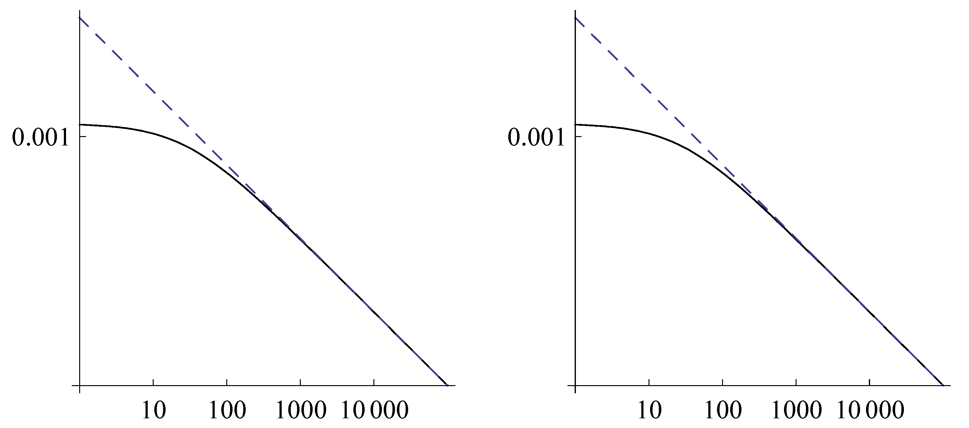
An asymptotic approximation of for large j is obtained by neglecting with respect to j and writing the first order expansion of for fixed . We get
where d is a suitable constant, showing that satisfies a power law. Function is a good approximation of for large j, as shown in Figure 1 where the log-log plots of (solid line) and of (dashed line) are given for two different choices of the parameters and .
The log-log representations of and are
where .
Note that is not solution of a mixed model. The case of the power law function will be taken up again in the next section.
2.5. The General Case
When dealing with real-world data, often improperly collected or contaminated by noise, superpositions of more different models defined in not overlapping intervals of j have been suggested. We prefer instead to consider a single model obtained by combining some basic functions.
In literature many different functions have been proposed. Some of them lead to solutions of a model , which implies a nonlinear ratio . In general, pairs which solve Equation (4) exactly are not immediately found. So, we suggest to choose some interesting and derive from them, as shown in Section 2.2.
In practice, is obtained by fitting given samples in the log-log space, i.e., by using its log-log representation
must be normalized in such a way that . To guarantee the convergence of the series, we must assume that has an asymptotic growth rate lower than .
Let us examine some important examples.
- The power law model, in which log-log function is a straight line
- The log-normal model, in which log-log function is a parabola
The log-normal solution coincides with the probability density function of the log-normal distribution, as can be seen by setting
- The cut-off model, in which log-log function is an exponential
- We suggest a unifying approach: the function is
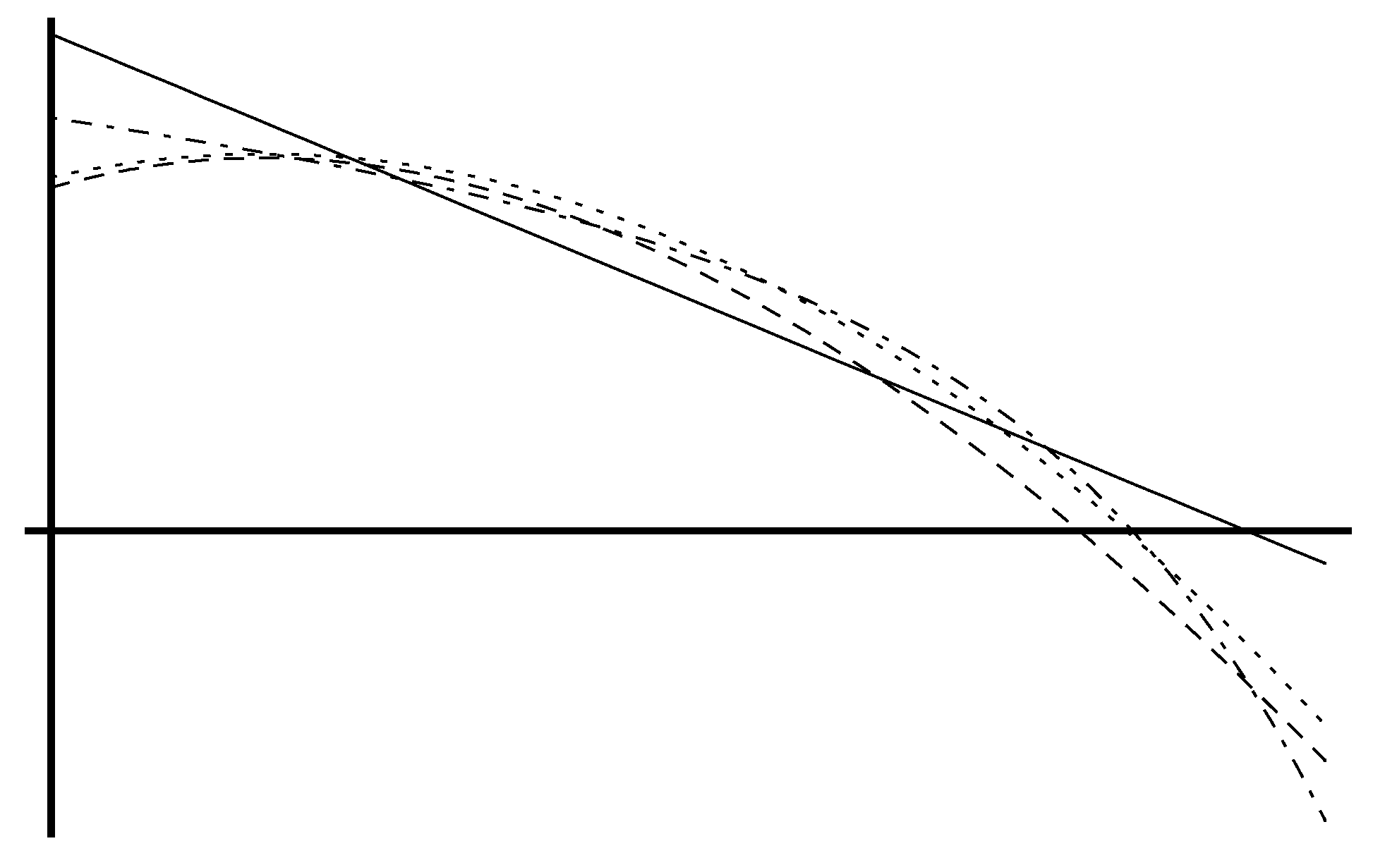
The exponential term is responsible of a faster decay of the solution with respect to the power law for large j, while the log terms are responsible for a bending down for small j. To show the different behaviors of the functions considered above, Figure 2 shows the log-log plots of (solid line), (dotted line), (dotted-dashed line), and (dashed line) obtained through a fitting procedure of a same dataset.
The probabilities corresponding to are derived as shown in Section 2.2, obtaining
The pair constitutes our proposed model, called cubic-cut-off. To get a better insight into the behavior of the model, it would be desirable to have an analytic expression for . Unfortunately, functions and which satisfy the recurrence (4) exactly, as in the case of the functions and defined in (13), are not easy to be given in a closed-form.
Hence, we settle for an approximation of . According to (22), should approximate . This suggests to express in the log-log scale with a basis similar to that used for . So, we assume for an expression of the form
where is a function of order lower than , and is a coefficient to be determined; then,
Now, we impose that the dominant terms of and in the asymptotic setting coincide. Since
it follows that . We postpone the choice of a suitable function to the next section, where a fitting technique is suggested. The validation of this procedure will be effectively checked by the experimentation.
The same technique allows finding also the probabilities corresponding to the log-normal and the cut-off functions.
3. Treatment of the Data
When data from real life phenomena are sampled and analyzed, intrinsic problems of various kind arise, namely:
- The crawling process through which data are acquired can produce complete or partial datasets. English Wikipedia-2018 is an example of a complete crawling, whereas English Web must inevitably be partially crawled.
- For the visualization of multi-scale data, a log-log plot is required, in order to better evidence the properties of the data and the possible correspondence with the chosen model. For example, if the chosen model is the power law, the log-log data should have a straight line representation.
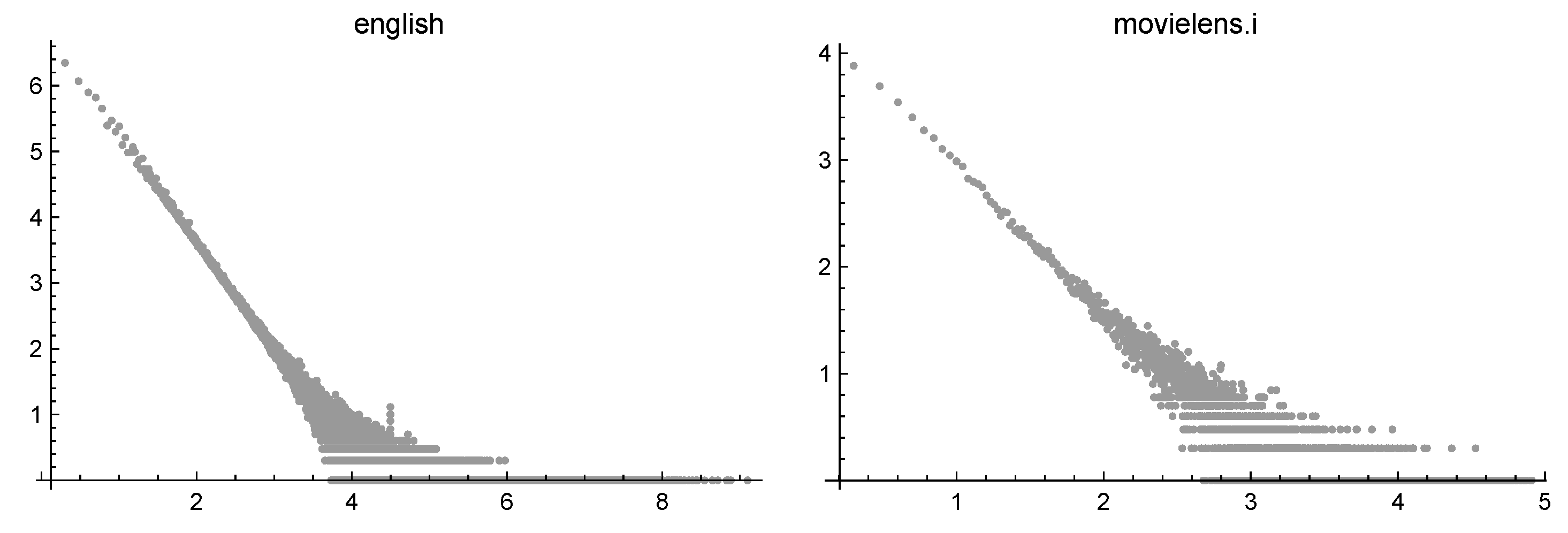
- In the previous sections, we looked for approximations of a function verifying for t large enough. Actually, when real-world phenomena (such as the web or the whole English language) are considered, t is so large that it can be assumed infinite. In practice, we deal with J samples , and, typically, the quantity is much smaller than t. So, we assumewhere d is a suitable scaling factor. Note that , being the number of items having degree j, is a nonnegative integer, while is a real number which can be very small. The quantization phenomenon cannot be considered statistical noise (as done by some authors) but is an intrinsic characteristic of the sampled data. For example, if , the corresponding values are mostly 0 but sometimes 1 or 2. Obviously, the zeros become more and more probable until the last data are reached.In the log-log scale, the values are gathered in plateaus on the tail of the dataset. Figure 3 shows the base 10 log-log representation of the frequencies of two datasets described in the next section: a set of English words and a set of MovieLens ratings. The quantization phenomenon is evident.
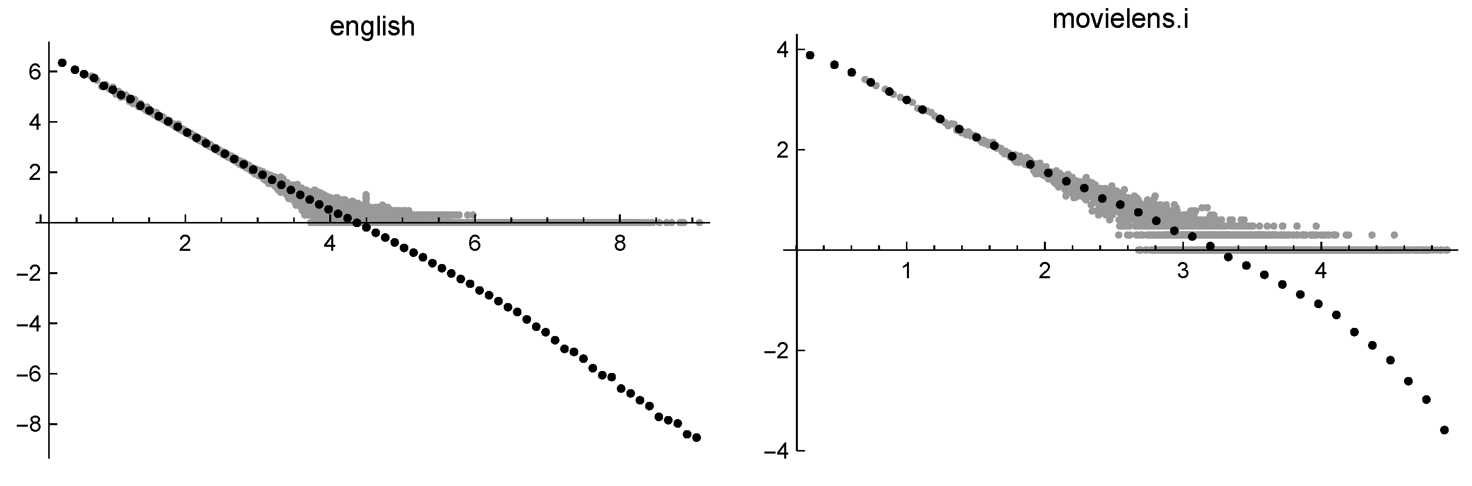
- A dequantization process can be accomplished by binning the data: the data values belonging to a given small interval (called a bin) are replaced by a value representative of that interval. When the binning is performed in the log-log scale, negative values might be generated. This procedure is essential to recover the asymptotic properties of the phenomenon and allows to reduce the size of data while performing some sort of smoothing. In Figure 4, the same data of Figure 3 are presented, together with the result of binning. It is clear that the binning reveals the different asymptotic behavior of the two data sets.
3.1. The Binning
We suggest the following logarithmic binning, which produces bins of equal width in the log-log scale.
Given , we consider the sequence , , where n is such that . The ith bin is for . The set Y of the binned data is formed by the pairs , where
If no point exists with , the pair is discarded (this may happen for large i). Note that, because of the discarded pairs, the set Y might have size lower than n, but, for simplicity, we still denote by n the size of Y. In the experimentation, has been tuned through a preliminary processing.
3.2. The Fitting
The fitting procedure is performed in the log-log plane on the binned data
Let be the cubic-cut-off function defined in (20):
We compute
imposing the constraint . For the other functions of Section 2.5, we compute the fit (25) setting to zero some coefficients of .
If , the solution is
In some cases, the coefficient might be zero. The series is convergent for , or, for , when . The corresponding model is derived according to (5):
We can give a closed-form approximation of the sequence through the function defined in (24). We have already suggested that coincides with the coefficient of the exponential term of , in the present case , but we still need to compute the function defined in (23).
In analogy with what has been done for , we try for a polynomial regression with degree 3. So, we consider a subset of integers , , in , equispaced in the logarithmic scale, such that and . Then, setting , and , we solve the minimum problem
Replacing in (23), we get
A specific performance index (31) controls the effectiveness of the similarity of to . A too large would raise doubts on the approximation, possibly due to numerical instability in the computation of .
3.3. The Attachment Rule
Instead of computing directly as the ratio between the sequences and for , the sequence can be approximated by a function obtained exploiting the closed-form approximation of :
The error of this approximation is measured by a specific performance index (32). If is sufficiently small, the investigation of for gives useful hints on . The quantity
satisfies
Then, we can assume as the probability for an attachment rule on the whole interval . The value has been excluded from definition (29) because the maximum of does not change when assumes its maximum in . Of course, if the function is decreasing in , the value obtained from (29) coincides with . The function takes the place of the coefficient s in (10). We call sublinear the attachment if , superlinear if , and pseudo-linear if .
The attachment exponent , as defined in (29), holds for the whole interval, but it depends excessively on the head of the dataset in which behavior, even though in agreement with our model, could generate a uselessly overestimated attachment rule. An attachment exponent less affected by the first points could be more indicative. To this aim, we restrict our computation of (29) to a subinterval which leaves out the first points (in our experimentation, we took ).
The quantity can be used as a possible numerical measure to discriminate different types of datasets.
3.4. Performance Indices
In the experimentation, the function used for the fitting has been chosen among all the functions taken into consideration in the previous sections. Let , with , denote one of the functions. The corresponding normalized are
- the Beta function defined in (16),
- the power law function defined in (17),
- the log-normal function defined in (18),
- the cut-off function defined in (19),
- the cubic-cut-off function defined in (21).
Least squares procedures solve the minimization problem (25), except for the Beta function which requires a procedure of non linear minimization (we used a Nelder-Mead procedure). The quality of the fitting is measured by the NRMSE (normalized root-mean-square error)
where and are the minimum and the maximum of the values for . Besides the error , the suitability of the model to the dataset can be measured by the scaling factor of (26). In the case of , if , the series does not converge, and, in practice, is given a very large value. The same thing can also occur when the series is convergent, but numerical instability prevents a correct computation. When is too large, we judge the model to be inadequate for that dataset. The symbol ∞ in the tables of the next section identifies this case.
Two more performance indices have emerged in the presentation of the whole fitting procedure.
- (1)
- The quality of the approximation of by is measured by the NRMSEwhere and are the minimum and the maximum of the values for .
- (2)
- A too large discrepancy between and suggests that the similarity of the bases used for , and cannot be assumed. This is measured by the NRMSEwhere and are the minimum and the maximum of the values for .
These two indices and have been evaluated for all the functions, but only the values obtained for the cubic-cut-off are reported in the next section.
4. Experiments
The experimentation has been performed with a 3.2 GHz 8-core Intel Xeon W processor machine using Mathematica version 12 and carried out on 21 datasets divided in three groups: scalar phenomena, directed graphs, and bipartite graphs. The code, together with the datasets not available elsewhere, can be downloaded from Reference [13]. For each dataset, the citation, a brief description, the number N of items, and the size S, equal to the total number of degrees, are given below.
Following the description, a first table summarizes the results of the experimentation. Columns 1–5 of the table show the errors of the solutions computed by the different procedures. The error is replaced by ∞ if the series does not converge. For the power law, this means that , i.e., a well-defined mean does not exist. The error is replaced by an * if it exceeds by three times the best error for the same dataset. Columns 6, 7 list the indices and of cubic-cut-off. Column 8 lists the exponent of the attachment rule defined in (29), where , with .
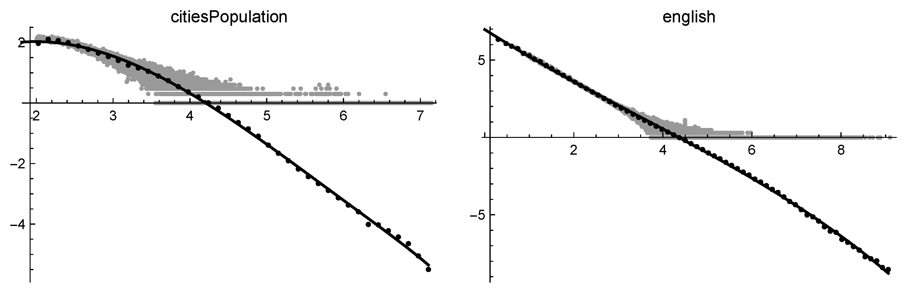
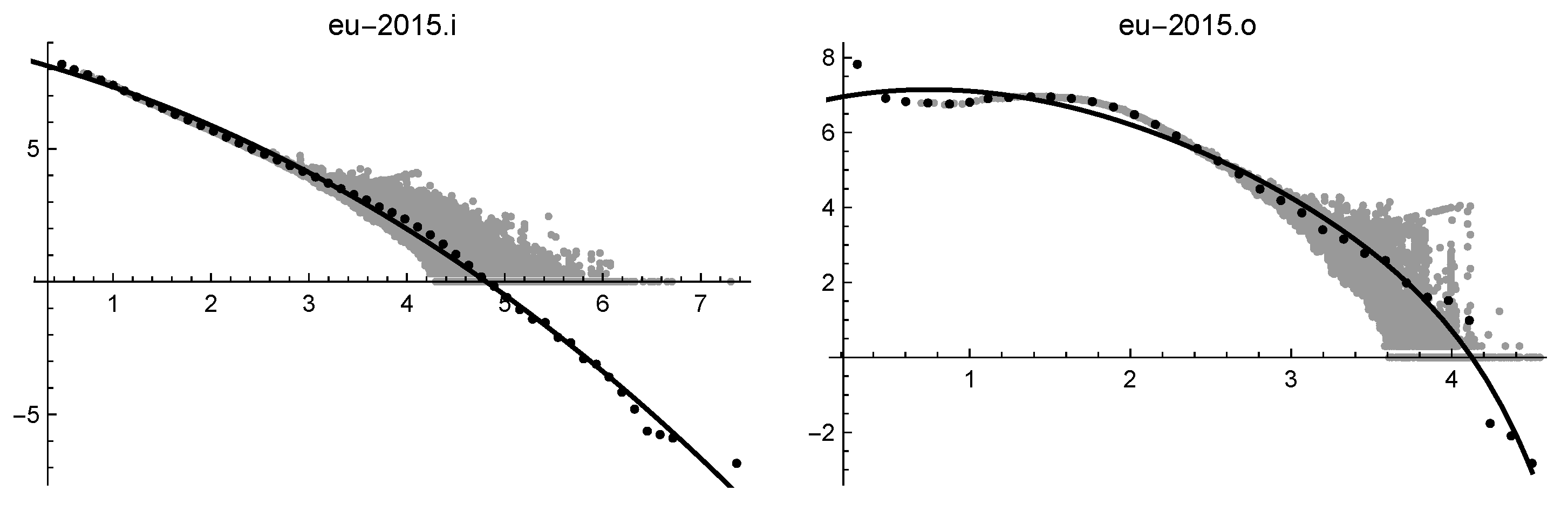
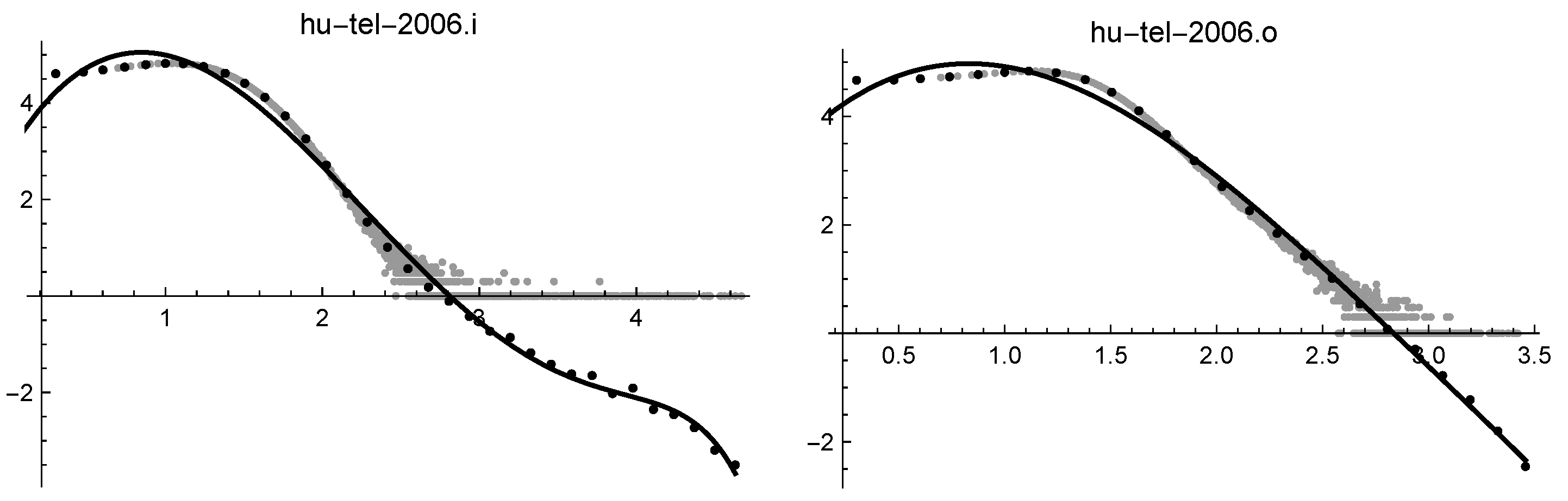
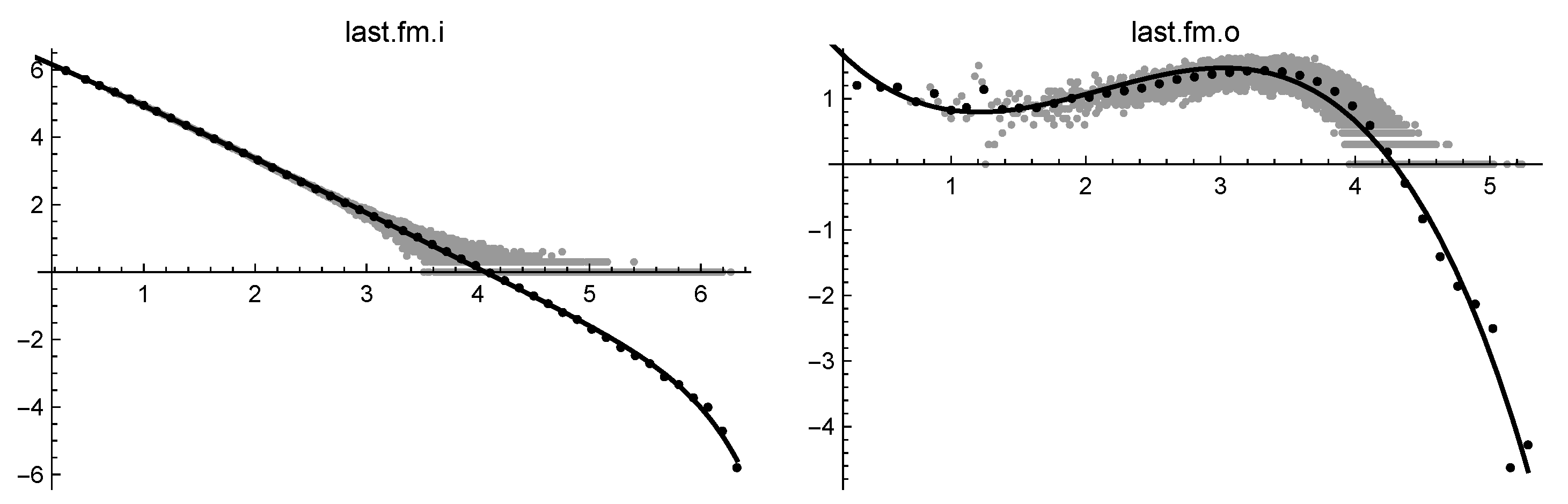
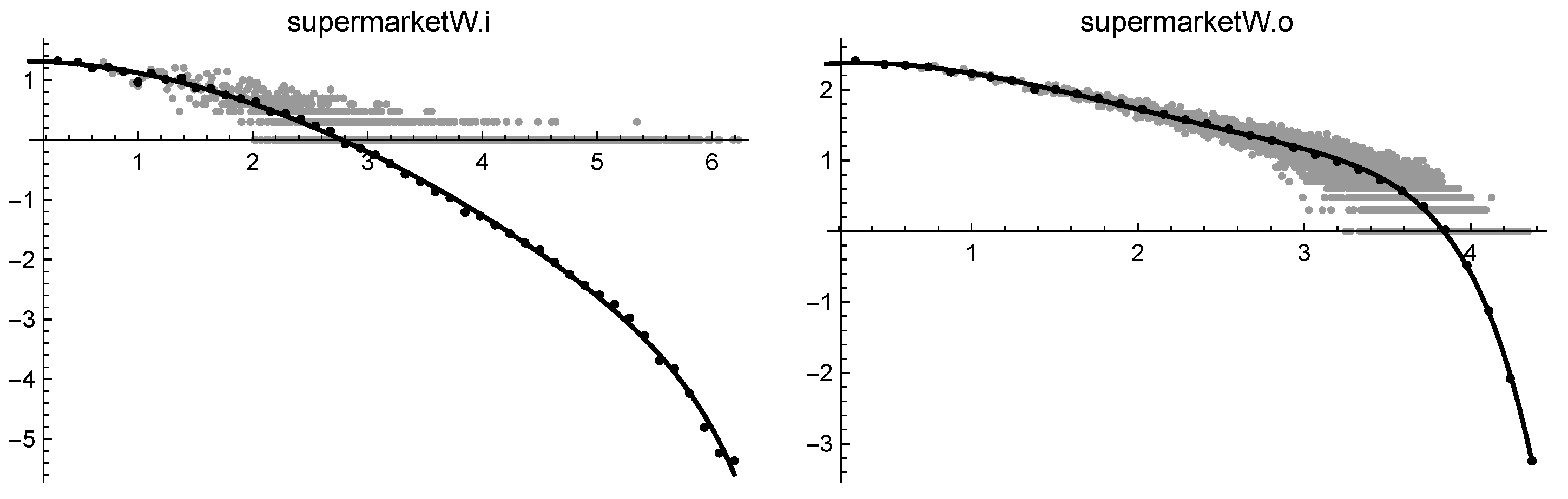
A second table gives the log-log representation of for some selected datasets. For these datasets, the base 10 log-log plots of the cubic-cut-off functions (solid line) are given, superimposed to the original data (gray points) and the binned data (black points). An integer i on the axis corresponds to in the linear scale.
4.1. Scalar Phenomena
The scalar phenomena are characterized by a single distribution of values. For each dataset, the file of the pairs , where is the frequency function defined in (1), is generated. The name of the file corresponds to the name of the dataset.
- cities population [14]. The population of N cities obtained by Mathematica CityData feature on February 2020. , and .
- english [15]. A large collection of English words obtained by joining a collection of Project Gutenberg texts and a collection of public USENET postings collected between October 2005 and January 2011. , and .
- hollywood-2011 [16]. One of the most popular social dataset: the graph of movie actors. Nodes are actors, and two actors are joined by a link whenever they appeared in a movie together. Since outdegree and indegree coincide, from the point of view of the frequency analysis, this is considered a scalar phenomenon. , and .
The errors of the computed solutions are given in Table 1.
4.2. Directed Graphs
In directed graphs, the edges have an orientation, so there exist inlinks (pointing to a node) and outlinks (originating from a node). In this case, the degree of the node becomes, more specifically, the indegree, which counts the inlinks, and the outdegree, which counts outlinks. For each graph, two files are generated with the frequency function (2): the one containing the indegrees and the one containing the outdegrees. Their names correspond to the name of the graph with the suffix .i and .o, respectively.
These datasets, except steemit, can be downloaded from Reference [16], where they have been stored compressed using LLP + WebGraph [17,18].
- clueweb12 [19]. The web graph underlying the ClueWeb12, a dataset created to support research on information retrieval and related human language technologies. , and .
- eu-2015 [20] The web graph of a large snapshot of the EU countries taken in 2015 by BUbiNG starting from the site http://europa.eu/. The maximum number of nodes per host was set to 10M (and never reached). , and .
- Wikipedia graphs [21]. The node connections for the following versions of Wikipedia: English (enwiki-2018) and , German (dewiki-2013) and , French (frwiki-2013) and , Spanish (eswiki-2013) and , and Italian (itwiki-2013) , and .
- hu-tel-2006 [16]. The social graph built from the detailed call record of Hungarian Telekom for an eight-month time frame in 2006. Measurements were performed by the Hungarian Academy of Sciences. , and .
- steemit [22]. The relations graph of Steemit, a blockchain-based blogging and social media website. , and .
- twitter-2010 [23]. The website, owned and operated by Twitter, Inc., which offers a social networking and microblogging service. Nodes are users, and there is an arc from x to y if y is a follower of x, i.e., the arcs follow the direction of the tweet transmission. , and .
The errors of the computed solutions are given in Table 3.
4.3. Bipartite Graphs
Bipartite graphs contain two types of nodes, active and passive. The edges connect an active node with a passive one. As in the previous case, for each graph, two files are generated with the frequency function (2): the one with the suffix .i contains the indegrees (i.e., the degrees of the passive nodes), and the one with the suffix .o contains the outdegrees (i.e., the degrees of the active nodes).
Most of the considered graphs are rating networks between persons and items they have rated. The ratings values are ignored, and only the information whether a person has rated an item is retained.
- book crossing [24]. Collected by Ziegler in a 4-week crawl (August/September 2004) from the Book-Crossing community. It contains the ratings about 271,379 books. , and .
- fine foods [25]. The dataset of the reviews of fine foods from Amazon. The data span a period of more than 10 years, up to October 2012. , and .
- last.fm. A large database of listening data crawled by [26] using the last.fm API. There were considered both relations user-song ( and ) and relations user-song weighted with the number of plays (, and ).
- movielens [27]. The dataset describes 5-star rating and free-text tagging activity from MovieLens, a movie recommendation service. It contains 25 M ratings. These data were created between 9 January 1995 and 21 November 2019. , and .
- supermarket. A small database of supermarket purchases collected by [28]. There were considered both relations user-product ( and ) and the relations user-product weighted with the number of purchases (, and ).
- Yahoo! artists [29]. The artists ratings collected from the Yahoo! Webscope dataset R1. This dataset represents a (anonymized) snapshot of the Yahoo! Music community’s preferences for various musical artists, collected in one month sometime prior to March 2004. , and .
The errors of the computed solutions are given in Table 5.
4.4. Comments
The first thing we note from Table 1, Table 3, and Table 5 is that cubic-cut-off mainly outperforms the other procedures, which could be so ranked: log-normal, Beta, cut-off, power law. The winning point of cubic-cut-off and log-normal is their better ability in adapting to the bending of the head, but log-normal behaves worse than cubic-cut-off in the tail because of the lack of the exponential term. The relevance of logarithmic terms is confirmed by the fact that, only in a small number of cases, cut-off reaches the performance of cubic-cut-off. The small values of e provide an indirect proof of the validity of the cubic-cut-off model.
From Table 3, we note a characteristic behavior of function of the cubic-cut-off for most directed graphs, in particular for Wikipedia graphs: typically, the indegree files have a larger attachment exponent than outdegree files. This agrees with the reasonable idea that the outlink processes are independent from the degree of the node, while the inlink process rely more on the degree of the node.
On the contrary, the difference between indegree and outdegree files in bipartite graphs appears reversed, pointing out the active role of a person in choosing a particular item. This is evident, for example, in the case of the supermarket datasets. We could try an explanation for these outcomes: it could be the result of some aggressive commercial policy which directs the purchases toward more advertised products. It is worth noting that cubic-cut-off succeeds in coping, even with the particularly difficult datasets last.fm.o and last.fmW.o, which exhibit a very messy head. In these cases, since the resulting attachment rule is conditioned by dozens of head points, it seems appropriate to let , thus reducing the exponent at values near 2.
A large attachment exponent appears for the citiesPopulation dataset, as well, pointing out the recognized great attractiveness of the most important cities of the world.
Finally, for many considered datasets, results decreasing in the tail, suggesting that the attachment rule might get weaker progressively when the items have a very large degree. If we associate the degree of an item to its age (as it is often made), in the sense that an item with a larger degree is assumed to be older, this weakening behavior could be considered as a possible indicator of a phenomenon of obsolescence.
5. Conclusions and Future Work
In this paper, a model for frequency analysis of systems representing multi-scale real-world phenomena has been proposed. At its basis, a discrete-time stochastic process leads to a steady state solution ruling the attachment policy. The attachment rule, which in the original mixed model is linear, has been enriched for including elements of the exponential cut-off model and of the log-normal model.
The proposed model, called cubic-cut-off, has been applied to a large number of datasets and results to be more effective than other models, like the widely applied log-normal and cut-off, which, in some cases, are unable to give acceptable approximations, as clearly appears from the inspection of Table 1, Table 3 and Table 5, where the cubic-cut-off is compared with the Beta function, the power law, the log-normal, and the cut-off.
In a few cases, its behavior is only a little better than the log-normal, showing that the cubic and exponential terms added to log-normal have a small influence, but, in most cases, the presence of these terms is essential to obtain good results.
The frequency analysis we performed in this paper applies to a network modeling based on graph representations as a discrete structure. The model we proposed belongs to the class of parametric models, where some finite set of parameters is assumed. Alternatively, the class of non-parametric models, where an infinite set of parameters is assumed, can be taken into consideration; see, for example, Reference [30], where a Bayesian non-parametric model for random graphs is proved to exhibit a power-law behavior, and a general framework for bipartite graphs, directed multigraphs, and undirected graphs is described. In future research, we are interested in studying non-parametric models applied to networks exhibiting peculiar behaviors, like the ones we considered in this paper.
Author Contributions
All the authors have contributed substantially and in equal measure to all the phases of the work reported. All authors have read and agreed to the published version of the manuscript.
Funding
This research received no external funding.
Conflicts of Interest
The authors declare no conflict of interest.
References
- Barabasi, A.L. Network Science; Cambridge University Press: Cambridge, UK, 2016. [Google Scholar] [CrossRef]
- Mitzenmacher, M. A Brief History of Generative Models for Power Law and Lognormal Distributions. Internet Math. 2003, 1, 226–251. [Google Scholar] [CrossRef] [Green Version]
- Adamic, L.A. Zipf, Power-Laws, and Pareto—A Ranking Tutorial; Information Dynamics Lab, HP Labs: Palo Alto, CA, USA, 2012; Available online: http://www.hpl.hp.com/research/idl/papers/ranking/ranking.html (accessed on 2 December 2020).
- Caldarelli, G.; De Los Rios, P.; Laura, L.; Leonardi, S.; Millozzi, S. A Study of Stochastic Models for the Web Graph; Technical Report 04-03; Dip. di Informatica e Sistemistica, Universita’ di Roma “La Sapienza”: Rome, Italy, 2003. [Google Scholar]
- Simon, H.A. On a Class of Skew Distribution Functions. Biometrika 1955, 42, 425–440. [Google Scholar] [CrossRef]
- Cooper, C.; Frieze, A.M. A general model of undirected web graphs. In European Symposium on Algorithms; Springer: Berlin/Heidelberg, Germany, 2001; pp. 500–511. [Google Scholar]
- Dorogovtsev, S.; Mendes, J.; Samukhin, A. Structure of Growing Networks: Exact Solution of the Barabasi-Albert’s model. Phys. Rev. Lett. 2000, 85, 4633–4636. [Google Scholar] [CrossRef] [Green Version]
- Pennock, D.M.; Flake, G.W.; Lawrence, S.; Glover, E.J.; Giles, C.L. Winners don’t take all: Characterizing the competition for links on the web. Proc. Natl. Acad. Sci. USA 2002, 99, 5207–5211. [Google Scholar] [CrossRef] [PubMed] [Green Version]
- Dereich, S.; Mörters, P. Random Networks with Sublinear Preferential Attachment: Degree Evolutions. Electron. J. Probab. 2009, 14, 1222–1267. Available online: https://projecteuclid.org/euclid.ejp/1464819504 (accessed on 11 December 2020). [CrossRef]
- Kunegis, J.; Blattner, M.; Moser, C. Preferential Attachment in Online Networks: Measurement and Explanations. arXiv 2013, arXiv:1303.6271. [Google Scholar]
- Abramowitz, M.; Stegun, I. Handbook of Mathematical Functions with Formulas, Graphs, and Mathematical Tables, National Bureau of Standards, 10th Printing; National Bureau of Standards (DOC): Washington, DC, USA, 1972.
- Beta Function. Available online: https://en.wikipedia.org/wiki/Beta_function (accessed on 2 December 2020).
- Supplementary Data for This Paper. Available online: http://pages.di.unipi.it/romani/MDPIdata.zip (accessed on 9 December 2020).
- Wolfram Language & System Documentation Center. Available online: https://reference.wolfram.com/language/ref/CityData.html (accessed on 4 December 2020).
- Project Gutenberg Literary Archive. Available online: ftp://mirrors.pglaf.org/mirrors/gutenberg-iso/pgdvd042010.iso (accessed on 4 December 2020).
- Laboratory for Web Algorithmics. Available online: http://law.di.unimi.it/datasets.php (accessed on 4 December 2020).
- Boldi, P.; Vigna, S. The Web Graph Framework I: Compression Techniques. In Proceedings of the 13th International Conference on World Wide Web, New York, NY, USA, 17–20 May 2004; ACM Press: New York, NY, USA, 2004; Volume 99, pp. 595–601. Available online: http://law.di.unimi.it/datasets.php (accessed on 4 December 2020).
- Boldi, P.; Rosa, M.; Santini, M.; Vigna, S. Layered Label Propagation: A MultiResolution Coordinate-Free Ordering for Compressing Social Networks. In Proceedings of the 20th International Conference on World Wide Web, Hyderabad, India, 28 March–1 April 2011; Srinivasan, S., Ramamritham, K., Kumar, A., Ravindra, M.P., Bertino, E., Kumar, R., Eds.; ACM Press: New York, NY, USA, 2011; pp. 587–596. [Google Scholar]
- ClueWeb12 Web Graph. Available online: http://www.lemurproject.org/clueweb12/webgraph.php/ (accessed on 4 December 2020).
- Boldi, P.; Marino, A.; Santini, M.; Vigna, S. BUbiNG: Massive Crawling for the Masses. In Proceedings of the Companion Publication of the 23rd International Conference on World Wide Web, Seoul, Korea, 7–11 April 2014; pp. 227–228. [Google Scholar]
- Boldi, P.; Codenotti, B.; Santini, M.; Vigna, S. Ubicrawler: A Scalable Fully Distributed Web Crawler. Software Pract. Exp. 2004, 34, 711–726. [Google Scholar] [CrossRef]
- Guidi, B.; Michienzi, A.; Ricci, L. A graph-based socio-economic analysis of Steemit. IEEE Trans. Comput. Soc. Syst. Submitted to.
- Kwak, H.; Lee, C.; Park, H.; Moon, S. What is Twitter, a Social Network or a News Media? In Proceedings of the 19th International World Wide Web (WWW) Conference, Raleigh, NC, USA, 26–30 April 2010; ACM Press: New York, NY, USA, 2010; pp. 591–600. [Google Scholar] [CrossRef] [Green Version]
- Ziegler, C.N.; McNee, S.M.; Konstan, J.A.; Lausen, G. Improving Recommendation Lists Through Topic Diversification. In Proceedings of the 14th International World Wide Web Conference (WWW ’05), Chiba, Japan, 10–14 May 2005. [Google Scholar]
- McAuley, J.; Leskovec, J. From Amateurs to Connoisseurs: Modeling the Evolution of User Expertise through Online Reviews. WWW 2013. Available online: https://snap.stanford.edu/data/web-FineFoods.html (accessed on 4 December 2020).
- Bradan, A.L. Forecast Emerging Artists Success on Last.fm Music Service: A Data-Driven Study. Master’s Thesis, University of Pisa, Pisa, Italy, 2020. [Google Scholar]
- Movie Lens. Available online: https://grouplens.org/datasets/movielens/ (accessed on 4 December 2020).
- Pennacchioli, D.; Coscia, M.; Rinzivillo, S.; Pedreschi, D.; Giannotti, F. Explaining the product range effect in purchase data. In Proceedings of the 2013 IEEE International Conference on Big Data, Big Data 2013, Santa Clara, CA, USA, 6–9 October 2013; pp. 648–656. [Google Scholar] [CrossRef]
- Yahoo! Webscope Dataset ydata-ymusic-user-artist-ratings-v1_0 Yahoo! Music User Ratings of Musical Artists, Version 1.0. Available online: http://webscope.sandbox.yahoo.com/catalog.php?datatype=r (accessed on 11 December 2020).
- Caron, F.; Fox, E.B. Sparse Graphs using Exchangeable Random Measures. J. R. Stat. Soc. Ser. B 2017, 79, 1295–1366. Available online: https://0-rss-onlinelibrary-wiley-com.brum.beds.ac.uk/doi/full/10.1111/rssb.12233 (accessed on 4 December 2020). [CrossRef] [PubMed] [Green Version]
Figure 1.
Log-log plots of (solid line) and of (dashed line), in the cases , (left) and , (right).

Figure 2.
Log-log plots of (solid line), (dotted line), (dotted-dashed line), and (dashed line).

Figure 3.
Frequencies of English words (on the left) and of MovieLens ratings (on the right).

Figure 4.
Binned frequencies of English words (on the left) and of MovieLens ratings (on the right).
Figure 4.
Binned frequencies of English words (on the left) and of MovieLens ratings (on the right).

Figure 5.
Log-log solutions of citiesPopulation (on the left) and of english (on the right).

Figure 6.
Log-log solutions of eu2015.i (on the left) and of eu2015.o (on the right).

Figure 7.
Log-log solutions of hutel2006.i (on the left) and of hutel2006.o (on the right).

Figure 8.
Log-log solutions of last.fm.i (on the left) and of last.fm.o (on the right).

Figure 9.
log-log solutions of supermarketW.i (on the left) and of supermarketW.o (on the right).


Table 1.
Errors and attachment exponents for scalar phenomena.
| File | ||||||||
|---|---|---|---|---|---|---|---|---|
| citiesPopulation | 0.015 | ∞ | 0.017 | * | 0.010 | 0.081 | 0.026 | 2.71 |
| english | * | ∞ | 0.010 | 0.012 | 0.005 | 0.016 | 0.004 | 1.17 |
| hollywood2011 | * | ∞ | * | * | 0.007 | 0.043 | 0.037 | 1.28 |
* The symbol is used to indicate that there is not element in this category.
Table 2.
Solutions of two selected scalar phenomena.
| citiesPopulation | |
| english |
Table 3.
Errors and attachment exponents for directed graphs.
| File | ||||||||
|---|---|---|---|---|---|---|---|---|
| clueweb12.i | 0.024 | 0.026 | 0.026 | ∞ | 0.018 | 0.011 | 0.058 | 1.09 |
| clueweb12.o | 0.065 | 0.098 | 0.048 | 0.039 | 0.033 | 0.047 | 0.051 | 1.12 |
| eu2015.i | 0.033 | 0.044 | 0.018 | 0.041 | 0.018 | 0.001 | 0.019 | 1.18 |
| eu2015.o | 0.065 | * | 0.043 | 0.051 | 0.034 | 0.019 | 0.011 | 1.34 |
| enwiki2018.i | 0.013 | * | 0.008 | * | 0.006 | 0.009 | 0.016 | 1.03 |
| enwiki2018.o | 0.020 | * | 0.022 | * | 0.009 | 0.060 | 0.026 | 0.96 |
| dewiki2013.i | 0.014 | * | 0.012 | 0.025 | 0.011 | 0.004 | 0.011 | 1.04 |
| dewiki2013.o | 0.027 | * | 0.026 | * | 0.018 | 0.063 | 0.037 | 0.96 |
| frwiki2013.i | 0.012 | * | 0.011 | 0.020 | 0.009 | 0.010 | 0.016 | 1.03 |
| frwiki2013.o | 0.023 | * | 0.028 | * | 0.012 | 0.071 | 0.031 | 1.01 |
| eswiki2013.i | 0.012 | 0.019 | 0.012 | 0.014 | 0.009 | 0.019 | 0.019 | 1.00 |
| eswiki2013.o | 0.073 | 0.115 | 0.060 | 0.087 | 0.050 | 0.108 | 0.061 | 0.90 |
| itwiki2013.i | 0.016 | 0.026 | 0.014 | 0.017 | 0.011 | 0.014 | 0.015 | 1.01 |
| itwiki2013.o | 0.044 | * | 0.023 | * | 0.017 | 0.056 | 0.030 | 0.98 |
| hutel2006.i | 0.060 | * | * | ∞ | 0.022 | 0.092 | 0.055 | |
| hutel2006.o | 0.028 | * | 0.033 | * | 0.019 | 0.072 | 0.046 | 0.91 |
| steemit.i | 0.026 | ∞ | 0.014 | * | 0.013 | 0.001 | 0.001 | 1.24 |
| steemit.o | 0.022 | ∞ | 0.017 | 0.023 | 0.015 | 0.013 | 0.019 | 1.19 |
| twitter2010.i | 0.025 | 0.043 | 0.018 | 0.037 | ∞ | – | – | – |
| twitter2010.o | 0.019 | 0.025 | 0.023 | 0.025 | 0.017 | 0.016 | 0.042 | 1.04 |
* The symbol is used to indicate that there is not element in this category.
Table 4.
Solutions of four selected directed graphs.
| eu2015.i | |
| eu2015.o | |
| hutel2006.i | |
| hutel2006.o |
Table 5.
Errors and attachment exponents for bipartite graphs.
| File | ||||||||
|---|---|---|---|---|---|---|---|---|
| bookCrossing.i | 0.030 | 0.038 | 0.028 | 0.035 | 0.028 | 0.001 | 0.001 | 0.90 |
| bookCrossing.o | 0.026 | 0.035 | 0.021 | 0.027 | 0.020 | 0.006 | 0.003 | 1.06 |
| fineFoods.i | 0.039 | 0.043 | 0.040 | 0.041 | 0.038 | 0.013 | 0.016 | 0.87 |
| fineFoods.o | 0.040 | * | 0.034 | 0.023 | 0.014 | 0.028 | 0.057 | 0.99 |
| last.fm.i | * | ∞ | * | 0.006 | 0.005 | 0.029 | 0.020 | 1.15 |
| last.fm.o | * | ∞ | 0.105 | 0.070 | 0.035 | 0.260 | 0.168 | 3.33 |
| last.fm W.i | * | ∞ | * | * | 0.002 | 0.025 | 0.026 | 1.22 |
| last.fm W.o | 0.136 | ∞ | 0.086 | 0.141 | 0.063 | 0.183 | 0.064 | 3.34 |
| movieLens.i | * | ∞ | * | 0.006 | 0.004 | 0.012 | 0.007 | 1.33 |
| movieLens.o | 0.029 | 0.065 | 0.034 | 0.056 | ∞ | – | – | – |
| supermarket.i | * | ∞ | 0.030 | 0.027 | 0.013 | 0.009 | 0.012 | 1.99 |
| supermarket.o | * | ∞ | * | * | 0.017 | 0.134 | 0.147 | 2.03 |
| supermarketW.i | * | ∞ | 0.022 | * | 0.011 | 0.011 | 0.010 | 2.02 |
| supermarketW.o | * | ∞ | * | 0.012 | 0.004 | 0.038 | 0.048 | 2.06 |
| yahooArtists.i | 0.036 | ∞ | 0.032 | 0.021 | 0.018 | 0.018 | 0.016 | 1.34 |
| yahooArtists.o | 0.081 | 0.097 | 0.084 | 0.092 | 0.077 | 0.074 | 0.024 | 1.09 |
* The symbol is used to indicate that there is not element in this category.
Table 6.
Solutions of four selected bipartite graphs.
| last.fm.i | |
| last.fm.o | |
| supermarketW.i | |
| supermarketW.o |
Publisher’s Note: MDPI stays neutral with regard to jurisdictional claims in published maps and institutional affiliations. |
© 2020 by the authors. Licensee MDPI, Basel, Switzerland. This article is an open access article distributed under the terms and conditions of the Creative Commons Attribution (CC BY) license (http://creativecommons.org/licenses/by/4.0/).
Share and Cite
MDPI and ACS Style
Favati, P.; Lotti, G.; Menchi, O.; Romani, F. A Model for the Frequency Distribution of Multi-Scale Phenomena. Information 2020, 11, 580. https://0-doi-org.brum.beds.ac.uk/10.3390/info11120580
AMA Style
Favati P, Lotti G, Menchi O, Romani F. A Model for the Frequency Distribution of Multi-Scale Phenomena. Information. 2020; 11(12):580. https://0-doi-org.brum.beds.ac.uk/10.3390/info11120580
Chicago/Turabian StyleFavati, Paola, Grazia Lotti, Ornella Menchi, and Francesco Romani. 2020. "A Model for the Frequency Distribution of Multi-Scale Phenomena" Information 11, no. 12: 580. https://0-doi-org.brum.beds.ac.uk/10.3390/info11120580
Note that from the first issue of 2016, this journal uses article numbers instead of page numbers. See further details here.