Improving the Performance of Multiobjective Genetic Algorithms: An Elitism-Based Approach


Department of Electronics, Information and Bioengineering, Politecnico di Milano, Via Ponzio 34/5, I-20133 Milan, Italy
*
Author to whom correspondence should be addressed.
†
These authors contributed equally to this work.
Information 2020, 11(12), 587; https://0-doi-org.brum.beds.ac.uk/10.3390/info11120587
Submission received: 25 November 2020
/
Revised: 14 December 2020
/
Accepted: 16 December 2020
/
Published: 18 December 2020
(This article belongs to the Special Issue Artificial Intelligence and Decision Support Systems)
Abstract
:Today, many complex multiobjective problems are dealt with using genetic algorithms (GAs). They apply the evolution mechanism of a natural population to a “numerical” population of solutions to optimize a fitness function. GA implementations must find a compromise between the breath of the search (to avoid being trapped into local minima) and its depth (to prevent a rough approximation of the optimal solution). Most algorithms use “elitism”, which allows preserving some of the current best solutions in the successive generations. If the initial population is randomly selected, as in many GA packages, the elite may concentrate in a limited part of the Pareto frontier preventing its complete spanning. A full view of the frontier is possible if one, first, solves the single-objective problems that correspond to the extremes of the Pareto boundary, and then uses such solutions as elite members of the initial population. The paper compares this approach with more conventional initializations by using some classical tests with a variable number of objectives and known analytical solutions. Then we show the results of the proposed algorithm in the optimization of a real-world system, contrasting its performances with those of standard packages.
1. Introduction
Multiobjective (MO) optimization is one of the most common tools developed in recent decades to support decision-making. It has been largely used to tackle problems in the domains of industrial design [1,2,3], financial risk management [4,5,6,7], water resources systems [8,9,10,11], energy decisions [12,13,14] and environmental policy making [15,16,17,18]. Its well-known advantage is not to force the evaluation of all the criteria into one common unit of measurement (usually, money) as required by cost-benefit analysis. On the other hand, its disadvantage is that it produces a set of nondominated solutions (Pareto frontier) that may be rather large when the number of criteria is more than two or three. This means that a more in-depth analysis is usually needed to reach a final compromise solution. On the other hand, the identification of the full Pareto frontier means that the space of relevant values of the objectives is completely revealed. This also clarifies what can be achieved in terms of an objective, when another is optimized, i.e., it shows what performance of each objective can be granted, whatever choice is taken within the nondominated (efficient) set of decisions. A further well-known property of the Pareto frontier is that it allows determining the trade-offs of each individual choice, namely the decrease of performance of the other objectives when one is improved along the frontier. These important positive characteristics are usually counterbalanced by the high computational burden that is needed for the determination of the solutions of a multiobjective problem. Such problems are often highly nonlinear and with many decision variables, which means they cannot be solved by simplex method, on the one side, nor by analytical optimization algorithms such as dynamic programming, on the other. Modern solution tools for these problems are thus based on evolutionary heuristics often mimicking some natural process [19,20,21]. Algorithms of this type comprise simulated annealing [22], ant colony optimization [23], and cuckoo search [24], but the most common is by far the class of genetic algorithms (GAs) [25]. They are a group of tools that make a solution evolve to a better one, following a process inspired by the natural evolution of living species. As natural evolution selects the fittest individuals to survive in a given environment, these algorithms try to evolve a set of initial solutions (initial population) towards the best ones, implementing the rules that govern natural selection. Coupled with a multiobjective setting, GAs have been used in many different applications and several tools are available for their implementation [26,27,28]. One of the most famous and widely used is NSGA-II [29], which is used in this paper to present an innovative search setting. Multiobjective GAs have in fact to solve a multiobjective problem themselves in that they need to trade-off the breath of the search (that requires changes in the current search direction) with the depth of the search (that requires to keep digging in the current direction). This dilemma is solved in slightly different ways in the currently available packages, mainly exploiting various formulations of the mutation mechanism [30,31,32,33,34], but they can hardly guarantee a complete spanning of the Pareto frontier. This paper addressees exactly this point and shows how a full definition of the frontier boundary can be obtained.
Before doing this, we revise the main features of GAs in the next Section 2, also introducing the way in which their performance can be measured. In Section 3, we present the basic idea of exploiting the elitism mechanism for the complete exploration of the frontier and the advantages of the approach to support decision-making. Section 4 presents the results of adopting the proposed method to a set of sample problems, the exact solution of which can be determined analytically. Section 5 shows the application to a real-world case and, finally, Section 6 provides a discussion and draws some conclusions.
2. Genetic Algorithms’ Operators and Performances Evaluation
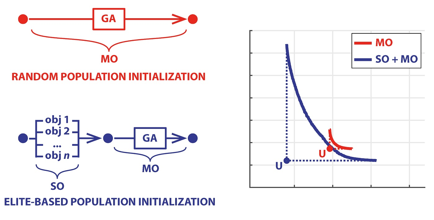
GAs try to replicate the natural selection process of a living population, defining how a series of processes take place (Figure 1). Given a population (of solutions) at a specific iteration step (which can be the initial one), a certain number of individuals is first selected. Some couples of these individuals are joined, forming new solutions with parts (genes) of the generating couple (crossover). The components of other individuals are randomly modified (mutation), and a new generation is defined. The purpose of all these actions is to determine the individuals that best perform in terms of the objective function, thus mimicking the Darwin principle of the “survival of the fittest”. The performance of any algorithm is therefore linked to the parameters and specific mechanisms with which each process (selection, crossover, mutation) is implemented. These mechanisms have to be set so that they ensure a proper balancing between diversity (exploration) and convergence (exploitation) [35,36,37,38].
To guarantee that the algorithm evolves toward the improvement of the objective function, the current best solutions are always moved to the following generation. This additional mechanism, called “elitism”, contributes significantly to the performance of the algorithm. It is, in fact, responsible for the depth of the search, whereas the other mechanisms determine its breath since they tend to enlarge the search space exploring at larger distances from the current best alternatives. The implementation of any GAs thus requires a careful selection of all these parameters and the standard approach is to test different combinations of their values. Further required assumptions are the dimension and composition of the initial population and the number of generations to compute. The last is the only parameter of the search algorithm that can be safely assessed by looking at the evolution of the objective function through the generations and stopping the algorithm when no gain is achieved for a certain number of iterations. Finally, since most of the above mechanisms are driven by random factors, it is customary to repeat the full procedure a number of times for each fixed set of parameter values.
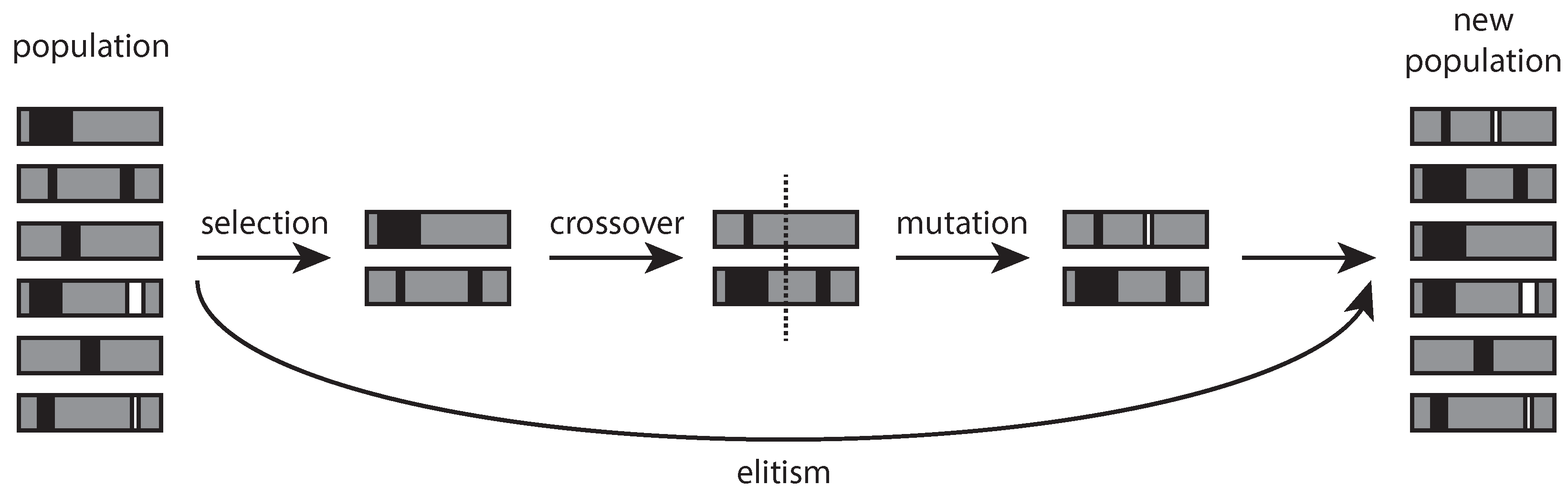
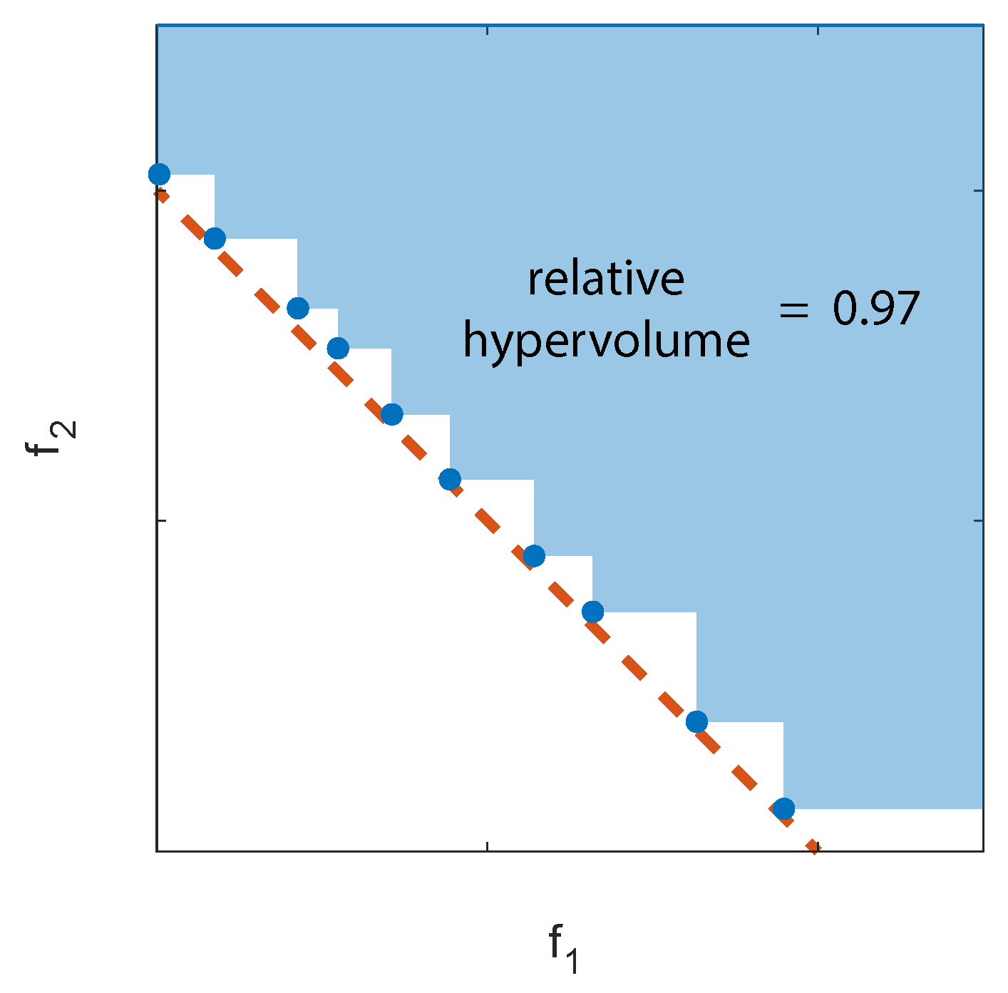
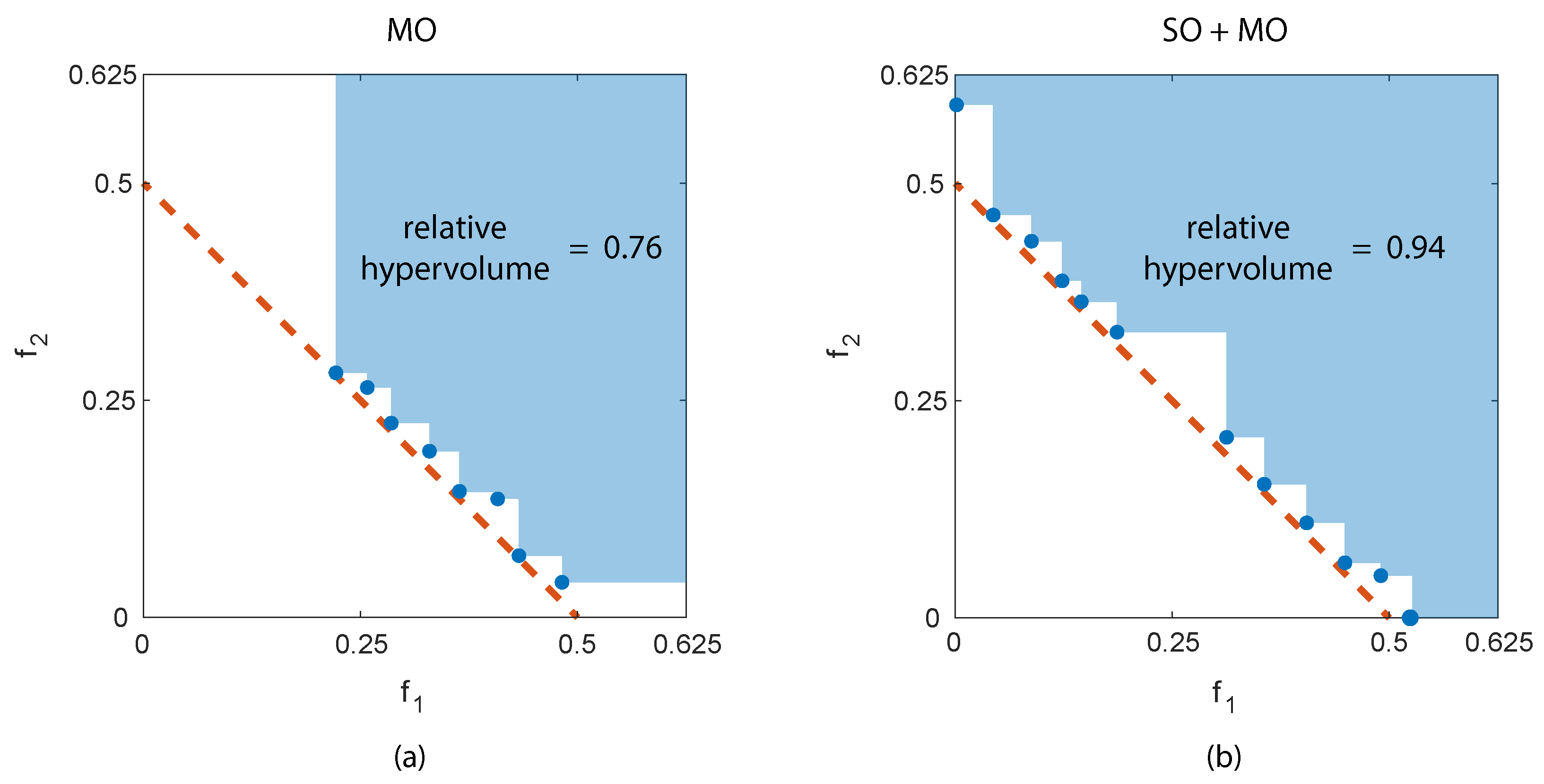
Measuring the performance of an algorithm in a multiobjective setting is not a trivial task. The problem solution is in fact constituted by the set of nondominated alternatives (i.e., those that cannot be improved under all the objectives at the same time) and thus one must determine how far the entire frontier moves. A way to measure this is to fix an arbitrary feasible solution in the objective space and determine the hypervolume explored by the algorithm [39]. The ratio between this portion of space and that delimited by a reference frontier is called “relative hypervolume” [40] as exemplified in Figure 2.
This reference frontier can be the exact one, when it is analytically known. In real-world cases, the actual Pareto frontier is unknown and this introduces a further bias in the definition of the hypervolume. One possible option is to assume, as a boundary, the set of all nondominated solutions determined by different algorithms, something that is clearly unreachable by each individual algorithm [41].
The numerical value of the hypervolume depends on the selected reference solutions (the frontier and the upper right corner in Figure 2). This means that the hypervolume is a suitable measure for the difference between two algorithms but its absolute value may not be very meaningful. In addition, selecting a too large reference volume may cause the differences between two algorithms to appear as irrelevant.
Finally, it is essential to remember that algorithms always work with discrete values and thus a complete spanning of a real continuous boundary is unfeasible unless an infinite number of iterations is possible. Therefore, even for a very efficient algorithm, the relative hypervolume is always below one, and the actual solution, when analyzed in detail, is always step-wise as exemplified in Figure 2 for the two-objective case.
3. Defining the Full Search Space
Most GAs propose and implement by default an initial random population. This choice is justified by the random nature of the evolution process and is particularly important when the domain of feasible values of the decisions is unknown. This is the case, for instance, when the decisions are the parameters of a model or a control rule, for which only non-negativity can be assumed. As said, this random initialization is repeated several times and a new elite fraction is determined at each initial step to guide the further search.
Considering an n-objective problem, we propose on the contrary to fix the initial elite fraction, in any repetition, by:
- First, solve separately n single-objective (SO) problems;
- Include the n optimal solutions (individuals) in the initial population of the MO problem;
- These solutions cannot be dominated and thus always remain in the elite set;
- Span the Pareto frontier with these solutions always in the population.
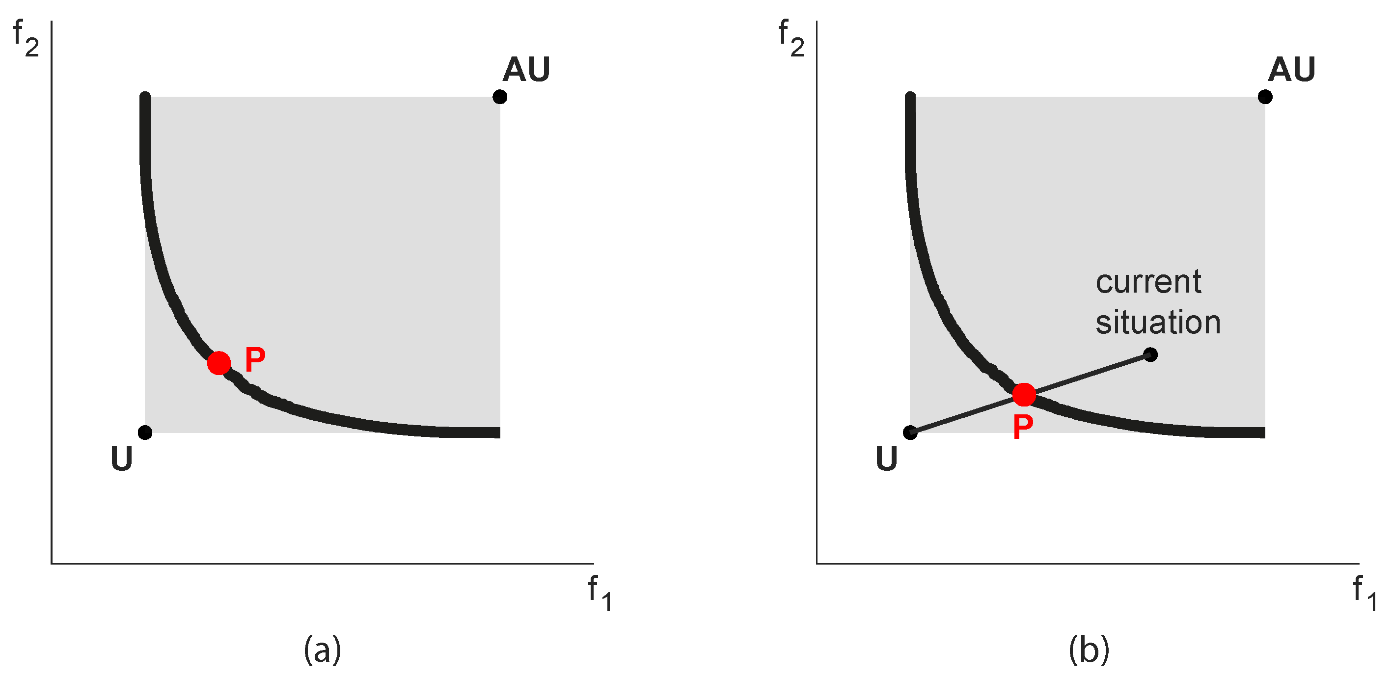
The n individual optimal solutions determine the so-called Utopia point (U), which defines the absolute best performance each objective can achieve. At the same time, it shows the guaranteed results of the other objectives, i.e., the values they can achieve even if only one objective is considered. These granted values determine a solution in the objective domain known as Anti-Utopia (AU). See again a two-objective example in Figure 3.
The Utopia and Anti-Utopia solutions are essential information for the negotiation among the stakeholders in all real-world problems. Indeed, they delimit the feasible and interesting space and show what are the maximum and minimum values of each objective that is reasonable to consider. There is no sense in discussing and trading outside these limits. Practical experience shows that, in some cases, the simple definition of this space is an important step to frame the discussion correctly and avoid fruitless litigation. Additionally, the definition of AU provides a clear reference for hypervolume calculations, and U constitutes an enlightening benchmark to suggest a specific nondominated solution in the Pareto frontier. Given that, in the end, a unique compromise solution (P) must be selected, decision-makers can be supported by determining the solution at minimum distance, suitably defined, from U (see Figure 3a). Or, when trying to define an improvement with respect to a current compromise solution (feasible by definition), one can select the intersection of the (hyper)segment connecting the current solution to U. In this way, each objective (possibly representing a specific stakeholder) can achieve the same proportion of the maximum achievable improvement (Figure 3b).
4. Analytical Tests
The proposed single-objective plus multiobjective (SO+MO) approach can be implemented on all GAs that allow for an external definition of the initial population, once the single-objective problems are separately solved. To show its effects in practice, we have used the Matlab implementation of the well-known and widely used NSGA-II algorithm [29] (function gamultiobj()), whose performance is traditionally considered as a benchmark. The standard GA algorithm in Matlab (function ga()) was also used for the single-objective step [42]. To fairly compare the two methods, we use the same number of function evaluations N, which defines the computational effort required to complete the optimization.
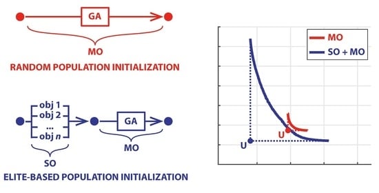
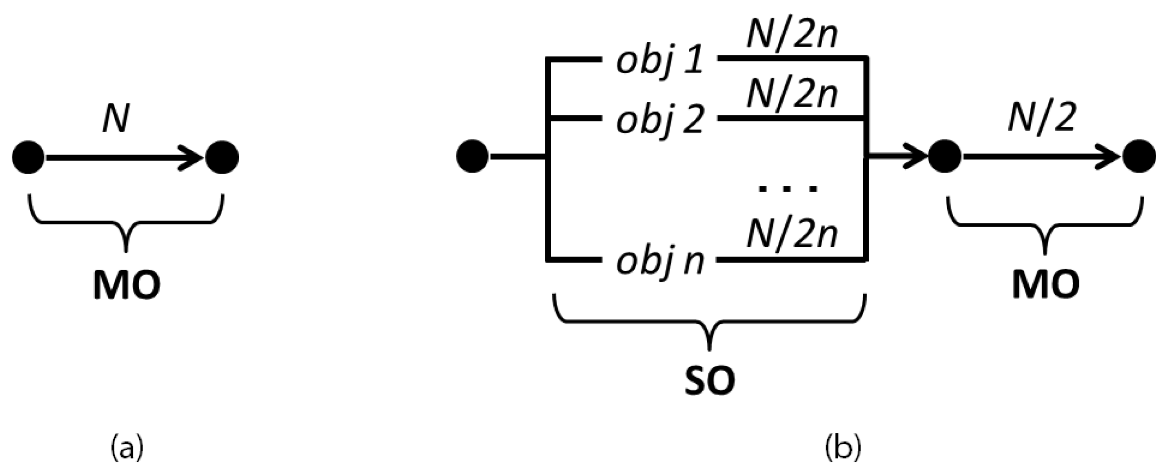
Figure 4 shows how the N function evaluations are assigned to the different steps of the traditional MO and of the proposed SO+MO methods. In the first, we directly solve the MO problem, and thus all the computation is reserved for that step. In the second, evaluations are reserved for the n SO problems, while the remaining evaluations for the final MO problem. How much to allocate to each task is a new parameter of the algorithm. In the following, has been assumed equal to , but this choice has proved to be not particularly critical in the experiments that follow.
In GAs, the number of function evaluations is defined as the product between the population size and the number of generations. The trade-off between a large population and many generations has been discussed in the GAs’ literature [43]. Large populations require more memory but, at the same time, allow speeding up the optimization, when the task is parallelized. In general, different combinations with the same number of function evaluations lead to similar results, provided that extreme situations are avoided. For instance, a single generation optimization (with a population size equal to the number of function evaluations) corresponds to a purely random search. Conversely, a population of few individuals is extremely inefficient even if the optimization lasts for many generations since it prevents the proper functioning of the evolutionary mechanisms. In this work, we consider a population size equal to the number of generations (equal to the square root of the number of function evaluations).
The performance of a GA is highly dependent on the initial population and the value assigned to the algorithm parameters, such as the probability of crossover and mutation, and the elite fraction, i.e., the individuals that are guaranteed to survive to the next generation. Finding the best combination of parameters for a heuristic is not easy and, given the strong random component, even if it would be possible, it is not guaranteed that the setting obtained considering a scenario will work equally well for a different set of input data. To take into account these issues, we defined a reasonable range for each parameter (i.e., crossover, mutation and elite fraction) and tested all the possible combinations. To avoid dependence on unlucky initial populations, 10 restarts with different random extractions have been performed for each parametrization.
We considered the two test problems introduced by Deb et al. [44] and traditionally used to evaluate the effectiveness of optimization algorithms [45]. These problems are scalable (i.e., arbitrary numbers of decision variables and objectives , m = 1,2,…,M, can be chosen), and the solutions are analytically known.
The following set of equations defines the test problem DTLZ #1:
In the objective space, the Pareto-optimal solutions of this problem lie on the hyperplane:
The following set of equations defines the test problem DTLZ #2:
The Pareto-optimal solutions of the problem defined by the set of Equation (3) lie on the following spherical surface in the objective space:
The above problems have a number of decision variables equal to . As suggested in the original paper [44], the parameter k has been fixed to 5 for # DTLZ1 and 10 for # DTLZ2.
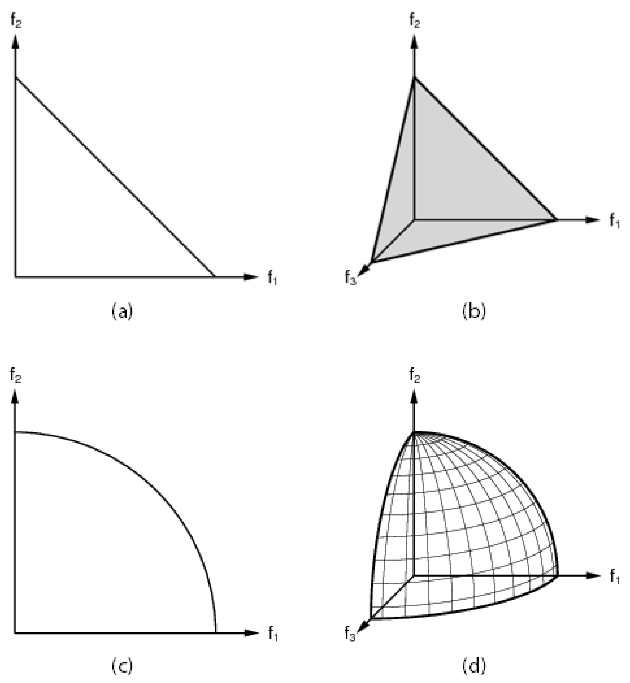
The 2D and 3D objective spaces for DTLZ #1 and #2 are represented in Figure 5.
As expected, the results obtained for problem DTLZ #1 strongly depend on the initial population. In some cases, the traditional MO with random initialization and the SO+MO approach provide an excellent approximation of the analytically known Pareto set with relative hypervolumes of the order of 0.95–0.96. Conversely, in other cases, the algorithms perform worse in two different ways. The randomly initialized MO algorithm is unable to fully explore the objective space and produces only a limited portion of the frontier (see Figure 6a) with relative hypervolume values of the order of 0.75. On the other side, the SO+MO approach is sometimes unable to provide an accurate determination of the entire Pareto set because the number of evaluation available for the MO step is reduced (Figure 6b). Nevertheless, the full breadth of the Pareto frontier is determined and, consequently, the relative hypervolume values continue to exceed 0.9. These results were obtained with thousands of evaluations (), half dedicated to the determination of the two separate optima of the two objectives and half to the MO step in the case of the proposed approach, all utilized for the MO evaluation in the other case.
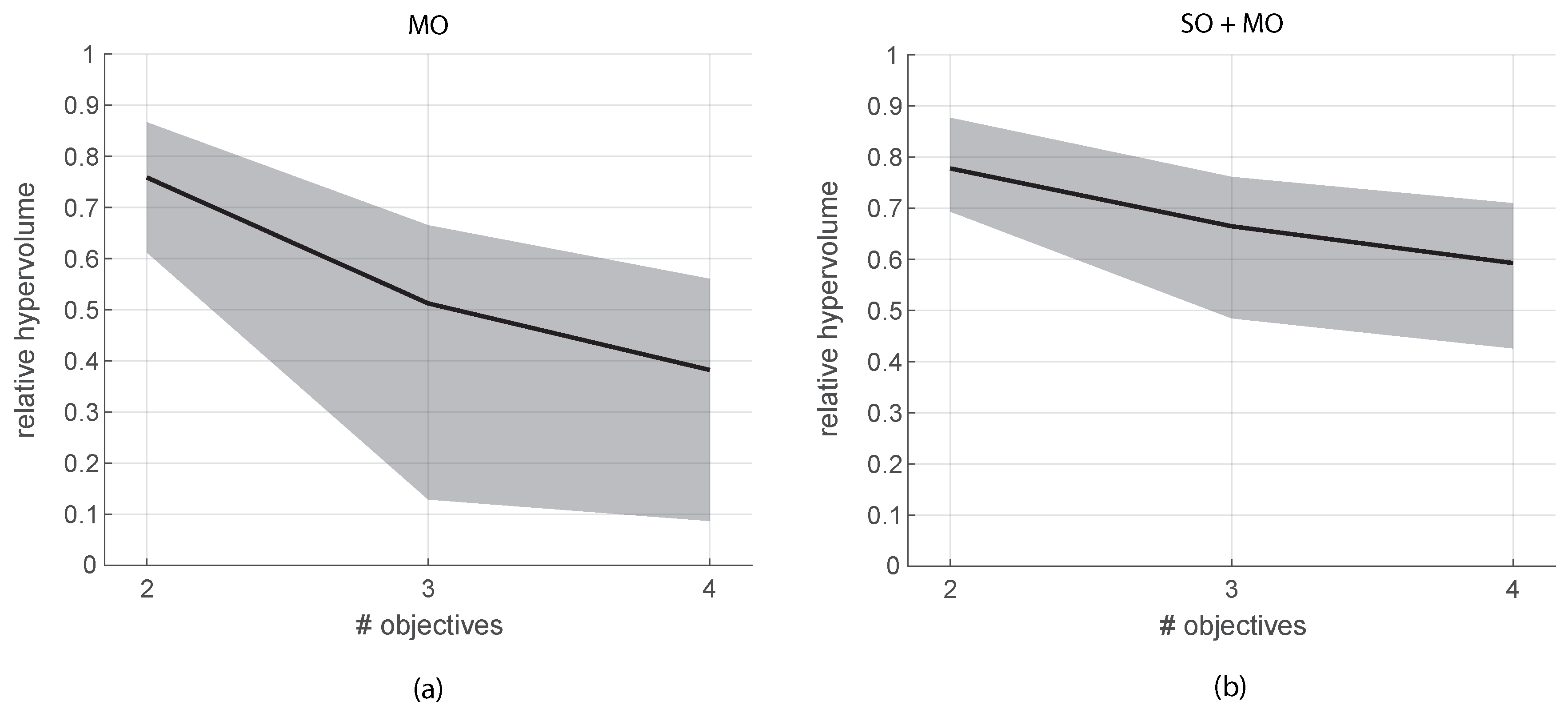
Initializing the elite set with the individual n SO solutions becomes more important when the number of objectives grows. Figure 7 illustrates the average relative hypervolume values (black line) for different numbers of objectives with the traditional initialization on the left (Figure 7a) and with the SO+MO approach on the right (Figure 7b). The grey band shows the variability of the values across all the repetitions. The function evaluations were for two objectives, for three objectives, and for four, always split half and half between the SO and the MO steps. It is evident that the proposed approach provides better average results and also guarantees a reduced variability of the approximation to the Pareto set. Note that the relative hypervolume values are all lower than in the preceding 2D case and are decreasing with the number of objectives. This is because, working in higher dimensions, the step-wise form of the numerical solution is more distant from the continuous analytical frontier. Nonetheless, it is evident that some random initialization may completely fail to approximate the correct solution, with relative hypervolume values that can go down to 0.1–0.2 already with three or four objectives. It is evident that the exact Pareto frontier is neither known nor continuous in real cases and thus the ability of an algorithm of guaranteeing certain performances is extremely important.
It is important to note that the way used to subdivide the computation adopted here (see, Figure 4) does not consider that the different SO problems generally have different complexity. Most of the times, a static splitting criterion can turn out to be suboptimal since it assigns the same number of function evaluations to easy (or lucky) as well as to complex (or unlucky) SO problems.
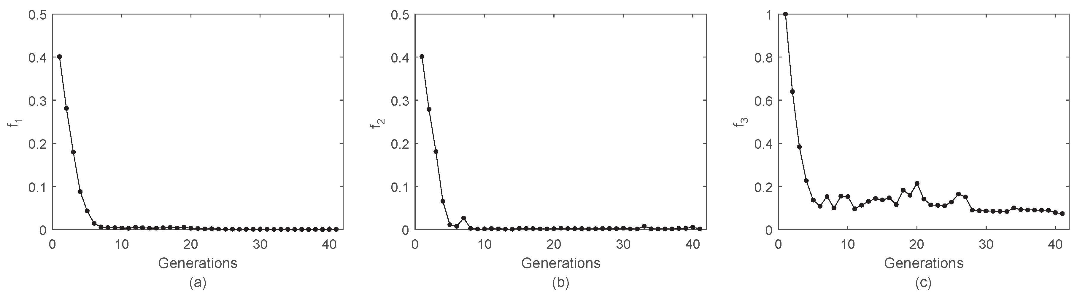
Considering as an example a 3-objective DTLZ #2 problem, the results of the SO optimization of and are sufficiently accurate after just a few generations (Figure 8a,b).
Conversely, is more critical, and its convergence slower (Figure 8c). However, in this case, our even splitting of the number of function evaluations reserved over 1600 evaluations for each SO problem, i.e., 40 generations, whereas only less than ten would have been sufficient. Note, additionally, that a very precise determination of the SO optima may not be necessary. The purpose of this step is to guide the following optimization, which will deep the search around the elite solutions anyway, so even a relatively rough estimation of the SO optima may still serve the purpose.
A possible strategy to further improve the algorithm efficiency consists of introducing a stopping criterion that saves unnecessary computation. A common choice, used by default in the Matlab optimization toolbox, is to stop the algorithm when the average value of the objective function, f, does not improve (considering a tolerance) for a given number of generations. This means that the user must define two additional parameters: the accepted tolerance and the number of generations that should satisfy the constraint before the algorithm stops.
5. Real-World Results
To further test the effectiveness of solving the preliminary SO problems before the final MO optimization, we considered a real-world water resources management case. The problem refers to the operation of the reservoirs in the Lower Nile River basin and has been extensively described in previous works [9,10].
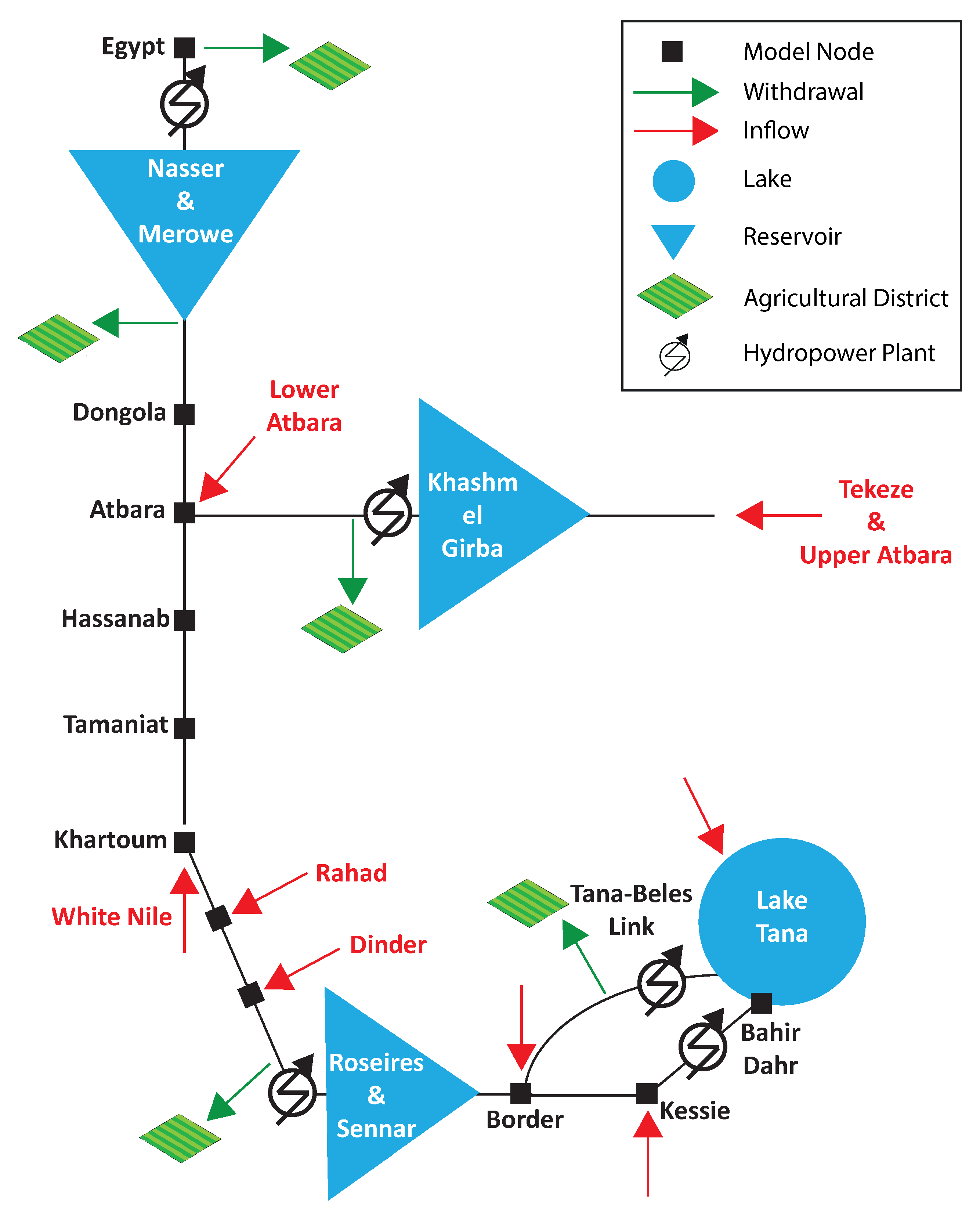
A schematic representation of the system is provided in Figure 9.
There are three artificial reservoirs and a natural lake at Lake Tana in Ethiopia. Two of the reservoirs represent the joint operations of two dams in cascade, Roseries and Sennar, in Sudan, and Merowe and Lake Nasser’s Aswan High Dam, between Sudan and Egypt. The other is Khashm el Girba reservoir on the Atbara River. These reservoirs’ combined storage capacity exceeds twice the average flow of 81.2 Gm as measured in Khartoum, Sudan. Downstream each water body, including Lake Tana, there is a hydropower station, for a total installed capacity of about 6 GW, one third of which at the outflow of Lake Nasser. Further downstream, there are agricultural districts that use the water for irrigation. These are largely dominated by the Egyptian agricultural demand that historically accounted for about two third of the Main Nile flow. Several of tributaries add water to the main flow at various junctions. The most important is the White Nile that joins the main river in Khartoum. It originates from the Central African catchment but reaches the junction with a relatively constant and low flow. Overall, the Nile flow shows a large interannual variability from about 90 to 140 Gm in dry and wet years, as well as a typical monthly pattern with minimum flow in spring at about 100 Mm per day and peaks in late summer-autumn at almost eight times as much. We assume that cooperation between states is possible (a very idealistic situation at the current time). So there are only two global objectives: average annual hydropower production and average yearly agricultural deficit. The first, , is defined as the annual average of all the power plants’ energy production. The energy generated in each plant is proportional to the product between the flow release through the turbines and the hydraulic head. The second objective, , is the annual average of the total water deficit, defined as the sum over all the agricultural districts of the positive differences between the monthly varying water demand and the water available in the same node at each monthly step. The two values and are rescaled for convenience into the range . Zero represents the best value of the objectives (full hydropower production and no agricultural deficit) and one the worst (zero hydropower and deficit equal to the demand). Both rescaled objectives must be minimized.
Each reservoir is characterized by its continuity equation:
where represents the storage at month t, is the release, the inflow, and the water losses, mainly due to evaporation, which is a nonlinear and time-varying function of the water storage. For instance, Lake Nasser’s surface may oscillate between about 1500 and 6500 km with monthly evaporation losses varying from 120 mm in January and about 300 in June, July, August, totaling an average annual loss of around 11–12 Gm, i.e., about 16% of the inflow to the lake. Additionally, each storage has a maximum and minimum value that force the release when these limits are hit. Once the releases are fixed, the water is run through the turbines (which again have a maximum capacity) for energy production and routed through the different branches of the system. Several additional inflows are received along this route, and water is abstracted for irrigation of the agricultural districts. These are supposed to derive an amount of water equal to their monthly varying requirements if the flow at their abstraction point is sufficient, otherwise they take less, and this causes the deficit. The simulation model implementing all these water balances at each point of the river system with a monthly time step has been built starting from [47,48]. Assuming the monthly release from each reservoir when all the water inflows are known as decision variables, their number depends on the number of years constituting the planning horizon. For instance, assuming a five-year scenario and monthly releases from three reservoirs, the number of decision variables is 180. The constraints necessary for problem definition in such a scenario are more than two hundred, and the nonlinearities are due to the equation of energy production, to the calculation of water evaporation, plus a number of thresholds (such as turbine capacity) that make the overall problem difficult to solve with algorithms different from GAs. After some testing, we selected the following parameters for NSGA-II. The initial population dimension was set to 2400, the number of restarts to 10, the elite fraction to 0.05 for SO, and to 0.35 for MO problems (the parameter ParetoFraction in the Matlab implementation). Crossover was set to 0.75. The execution time of each scenario on a 32-processor server (model Intel Xeon E5-2630L 1.80 GHz) was about 10 min. Again we used the same number of model evaluations for the random initialization (MO) and the SO+MO approach, splitting them into half and half. Given that a very long synthetic sequence of all inflows is available [48], many different five-year scenarios can be explored, each characterized by a different realization of the inflow process (red arrows in Figure 9).
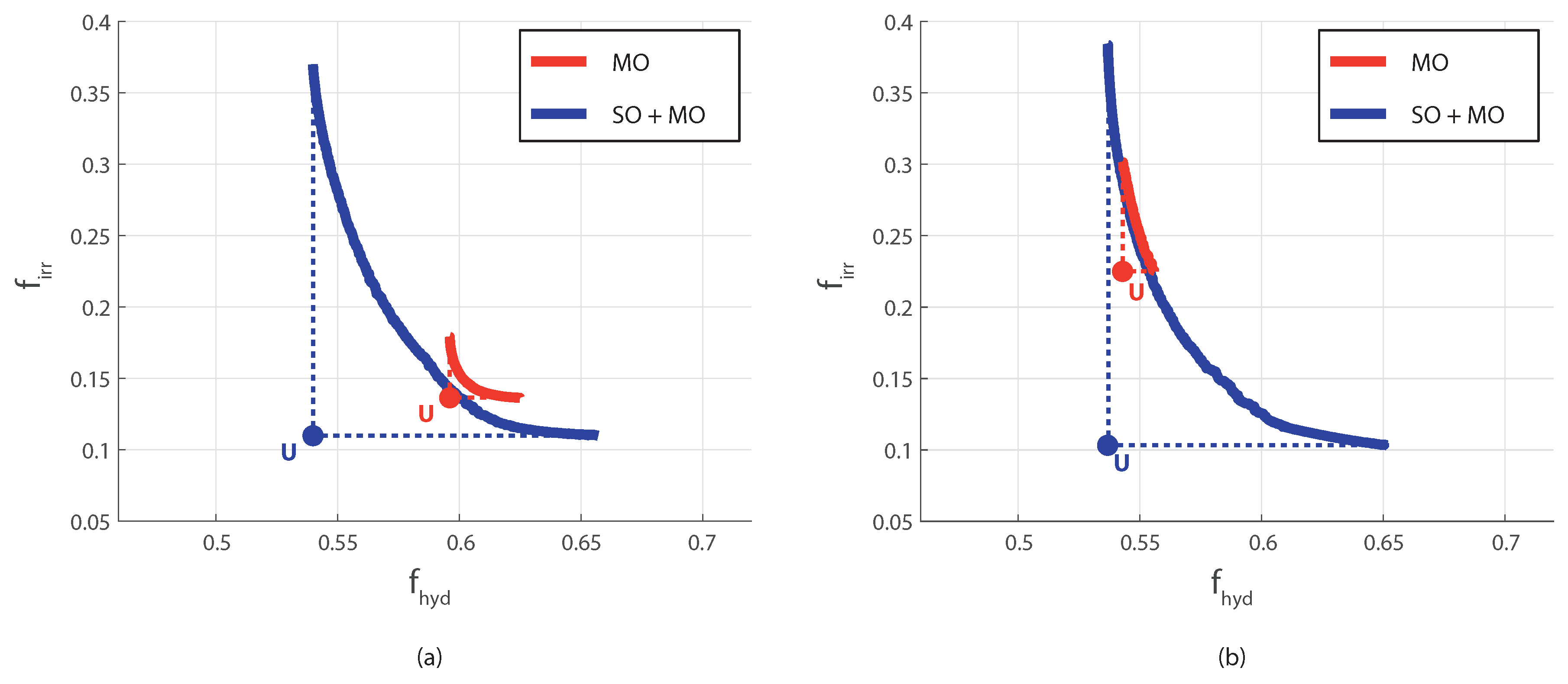
Sample results for two different scenarios are illustrated in Figure 10. They show that solving the MO problem with random initialization may not allow spanning the Pareto front properly also in this case.
In the case shown in Figure 10a, the random initialization ends up determining a poor approximation of the Pareto frontier that is dominated by that obtained with the proposed approach. It spans a very limited range of the objectives. This implies an erroneous determination of the Utopia point, which corresponds to the Pareto frontier’s extremes, by definition. In the other scenario (Figure 10b) the approximation is more precise. Still, it covers a narrow portion of the nondominated set, again determining a wrong position of the Utopia point with the consequences already mentioned in the negotiation between stakeholders. In both cases, even assuming that the real Pareto frontier is farther apart from that determined by the SO+MO approach, the solution obtained by the random initialization has a hypervolume that is just a fraction of that obtained with the proposed approach. The second attractive characteristic of the method, already seen in the analytical tests, emerges again here. The Pareto frontier determined by the SO+MO procedure is almost identical in the two scenarios that are samples of the same inflow time-series. On the contrary, the random initialization may lead to quite different and less robust results in different scenarios, even when they have the same statistical properties.
Many other approaches to the multireservoir management problem are possible and have been explored in a vast body of literature (see, for instance, ref [10] for the specific case of the Nile). We tested in particular the use of NSGA-II in the synthesis of reservoir control rules. In this case, the decision variables are the parameters of the assumed rule (from a few to hundreds, depending upon the assumed analytical form of the rule) and they are determined optimizing the same two objectives described above. The entire inflow sequence is used in this approach and only one Pareto frontier is determined. In addition, when taking this quite different management perspective, the random initialization of the GA prevents a complete definition of the boundary.
6. Conclusions
In contrast to the classical random initialization of MO GAs, the proposed approach uses the optimal values of the separate single-objective problems as elite members of the initial population. Given the elitist mechanism used in most GAs, they remain (with high probability) in the elite set along the entire search process, allowing a more correct spanning of the Pareto frontier. Extensive testing with analytical and real-world multiobjective optimization problems, encompassing different numbers of objectives and decision variables varying from very few to hundreds, demonstrated the procedure’s effectiveness. It helps solve test problems (DTLZ #1 and #2) more efficiently, especially when considering many objectives, and allows a better definition of crucial elements to support the negotiation process among different objectives/stakeholders. The real-world case shows, in fact, that relying on the standard (random) initialization may produce misleading indications.
The results reported above refer to the classical NSGA-II algorithm, but the proposed strategy could be implemented in other advanced MOGA solvers like BORG MOEA [49,50]. Further improvements are also possible, by carefully selecting the number of evaluations dedicated to the SO optimization and that used for the MO one. Depending on the specific characteristics of the algorithm under consideration, and on the ability to solve single-objective problems, the number of evaluations of the SO step may be reduced, thus achieving a higher speed while preserving a sufficient accuracy in the definition of the nondominated frontier.
Author Contributions
Conceptualization, G.G. and M.S.; methodology, G.G. and M.S.; software, M.S.; formal analysis, G.G. and M.S.; writing—original draft preparation, G.G. and M.S.; writing—review and editing, G.G. and M.S. All authors have read and agreed to the published version of the manuscript.
Funding
This research received no external funding.
Conflicts of Interest
The authors declare no conflict of interest.
References
- Rajesh, J.; Gupta, S.; Rangaiah, G.; Ray, A. Multi-objective optimization of industrial hydrogen plants. Chem. Eng. Sci. 2001, 56, 999–1010. [Google Scholar] [CrossRef]
- Ayala, H.V.H.; dos Santos Coelho, L. Tuning of PID controller based on a multiobjective genetic algorithm applied to a robotic manipulator. Expert Syst. Appl. 2012, 39, 8968–8974. [Google Scholar] [CrossRef]
- Nisi, K.; Nagaraj, B.; Agalya, A. Tuning of a PID controller using evolutionary multi objective optimization methodologies and application to the pulp and paper industry. Int. J. Mach. Learn. Cybern. 2019, 10, 2015–2025. [Google Scholar] [CrossRef]
- Tapia, M.G.C.; Coello, C.A.C. Applications of multi-objective evolutionary algorithms in economics and finance: A survey. In Proceedings of the 2007 IEEE Congress on Evolutionary Computation, Singapore, 25–28 September 2007; pp. 532–539. [Google Scholar]
- Bevilacqua, V.; Pacelli, V.; Saladino, S. A novel multi objective genetic algorithm for the portfolio optimization. In Proceedings of the International Conference on Intelligent Computing, Zhengzhou, China, 11–14 August 2011; pp. 186–193. [Google Scholar]
- Pai, G.V.; Michel, T. Metaheuristic multi-objective optimization of constrained futures portfolios for effective risk management. Swarm Evol. Comput. 2014, 19, 1–14. [Google Scholar] [CrossRef]
- Srinivasan, S.; Kamalakannan, T. Multi criteria decision making in financial risk management with a multi-objective genetic algorithm. Comput. Econ. 2018, 52, 443–457. [Google Scholar] [CrossRef]
- Giuliani, M.; Quinn, J.D.; Herman, J.D.; Castelletti, A.; Reed, P.M. Scalable multiobjective control for large-scale water resources systems under uncertainty. IEEE Trans. Control. Syst. Technol. 2017, 26, 1492–1499. [Google Scholar] [CrossRef]
- Sangiorgio, M.; Guariso, G. NN-based implicit stochastic optimization of multi-reservoir systems management. Water 2018, 10, 303. [Google Scholar] [CrossRef] [Green Version]
- Guariso, G.; Sangiorgio, M. Performance of Implicit Stochastic Approaches to the Synthesis of Multireservoir Operating Rules. J. Water Resour. Plan. Manag. 2020, 146, 04020034. [Google Scholar] [CrossRef]
- Guariso, G.; Sangiorgio, M. Spanning the Pareto Frontier of Environmental Problems. In Proceedings of the 10th International Congress on Environmental Modeling and Software, Brussels, Belgium, 14–18 September 2020. [Google Scholar]
- Yu, W.; Li, B.; Jia, H.; Zhang, M.; Wang, D. Application of multi-objective genetic algorithm to optimize energy efficiency and thermal comfort in building design. Energy Build. 2015, 88, 135–143. [Google Scholar] [CrossRef]
- Lu, Y.; Wang, S.; Zhao, Y.; Yan, C. Renewable energy system optimization of low/zero energy buildings using single-objective and multi-objective optimization methods. Energy Build. 2015, 89, 61–75. [Google Scholar] [CrossRef]
- Guariso, G.; Sangiorgio, M. Multi-objective planning of building stock renovation. Energy Policy 2019, 130, 101–110. [Google Scholar] [CrossRef]
- Hamarat, C.; Kwakkel, J.H.; Pruyt, E.; Loonen, E.T. An exploratory approach for adaptive policymaking by using multi-objective robust optimization. Simul. Model. Pract. Theory 2014, 46, 25–39. [Google Scholar] [CrossRef]
- Guariso, G.; Sangiorgio, M. Integrating Economy, Energy, Air Pollution in Building Renovation Plans. IFAC-PapersOnLine 2018, 51, 102–107. [Google Scholar] [CrossRef]
- Mayer, M.J.; Szilágyi, A.; Gróf, G. Environmental and economic multi-objective optimization of a household level hybrid renewable energy system by genetic algorithm. Appl. Energy 2020, 269, 115058. [Google Scholar] [CrossRef]
- Guariso, G.; Sangiorgio, M. Valuing the Cost of Delayed Energy Actions. IFAC-PapersOnLine 2020, in press. [Google Scholar]
- Deb, K. Multi-Objective Optimization Using Evolutionary Algorithms; John Wiley & Sons: Hoboken, NJ, USA, 2001; Volume 16. [Google Scholar]
- Yang, X.S. Review of meta-heuristics and generalised evolutionary walk algorithm. Int. J. Bio-Inspired Comput. 2011, 3, 77–84. [Google Scholar] [CrossRef]
- Beheshti, Z.; Shamsuddin, S.M.H. A review of population-based meta-heuristic algorithms. Int. J. Adv. Soft Comput. Appl. 2013, 5, 1–35. [Google Scholar]
- Du, K.L.; Swamy, M. Simulated annealing. In Search and Optimization by Metaheuristics; Springer: Berlin/Heidelberg, Germany, 2016; pp. 29–36. [Google Scholar]
- Dorigo, M.; Stützle, T. Ant colony optimization: Overview and recent advances. In Handbook of Metaheuristics; Springer: Berlin/Heidelberg, Germany, 2019; pp. 311–351. [Google Scholar]
- Rajabioun, R. Cuckoo optimization algorithm. Appl. Soft Comput. 2011, 11, 5508–5518. [Google Scholar] [CrossRef]
- Lee, C.K.H. A review of applications of genetic algorithms in operations management. Eng. Appl. Artif. Intell. 2018, 76, 1–12. [Google Scholar] [CrossRef]
- Houck, C.R.; Joines, J.; Kay, M.G. A genetic algorithm for function optimization: A Matlab implementation. Ncsu-ie tr 1995, 95, 1–10. [Google Scholar]
- Purohit, G.; Sherry, A.M.; Saraswat, M. Optimization of function by using a new MATLAB based genetic algorithm procedure. Int. J. Comput. Appl. 2013, 61, 15. [Google Scholar]
- Sheppard, C. Genetic Algorithms with Python, Smashwords ed.; CreateSpace Independent Publishing Platform: Charleston, SC, USA, 2017. [Google Scholar]
- Deb, K.; Pratap, A.; Agarwal, S.; Meyarivan, T. A fast and elitist multiobjective genetic algorithm: NSGA-II. IEEE Trans. Evol. Comput. 2002, 6, 182–197. [Google Scholar] [CrossRef] [Green Version]
- Ursem, R.K. Diversity-guided evolutionary algorithms. In Proceedings of the International Conference on Parallel Problem Solving from Nature, Granada, Spain, 7–11 September 2002; pp. 462–471. [Google Scholar]
- Chen, C.M.; Chen, Y.p.; Zhang, Q. Enhancing MOEA/D with guided mutation and priority update for multi-objective optimization. In Proceedings of the 2009 IEEE Congress on Evolutionary Computation, Trondheim, Norway, 18–21 May 2009; pp. 209–216. [Google Scholar]
- Tan, K.C.; Chiam, S.C.; Mamun, A.; Goh, C.K. Balancing exploration and exploitation with adaptive variation for evolutionary multi-objective optimization. Eur. J. Oper. Res. 2009, 197, 701–713. [Google Scholar] [CrossRef]
- Liagkouras, K.; Metaxiotis, K. A new probe guided mutation operator for more efficient exploration of the search space: An experimental analysis. Int. J. Oper. Res. 2016, 25, 212–251. [Google Scholar] [CrossRef]
- Kesireddy, A.; Carrillo, L.R.G.; Baca, J. Multi-Criteria Decision Making-Pareto Front Optimization Strategy for Solving Multi-Objective Problems. In Proceedings of the 2020 IEEE 16th International Conference on Control & Automation (ICCA), Singapore, 9–11 October 2020; pp. 53–58. [Google Scholar]
- Laumanns, M.; Thiele, L.; Deb, K.; Zitzler, E. Combining convergence and diversity in evolutionary multiobjective optimization. Evol. Comput. 2002, 10, 263–282. [Google Scholar] [CrossRef]
- Zhao, G.; Luo, W.; Nie, H.; Li, C. A genetic algorithm balancing exploration and exploitation for the travelling salesman problem. In Proceedings of the 2008 Fourth International Conference on Natural Computation, Jinan, China, 18–20 October 2008; Volume 1, pp. 505–509. [Google Scholar]
- Črepinšek, M.; Liu, S.H.; Mernik, M. Exploration and exploitation in evolutionary algorithms: A survey. ACM Comput. Surv. (CSUR) 2013, 45, 1–33. [Google Scholar] [CrossRef]
- Hussain, A.; Muhammad, Y.S. Trade-off between exploration and exploitation with genetic algorithm using a novel selection operator. Complex Intell. Syst. 2019, 6, 1–14. [Google Scholar] [CrossRef] [Green Version]
- Zitzler, E.; Thiele, L. Multiobjective optimization using evolutionary algorithms—A comparative case study. In Proceedings of the International Conference on Parallel Problem Solving from Nature, Amsterdam, The Netherlands, 27–30 September 1998; pp. 292–301. [Google Scholar]
- Bader, J.; Deb, K.; Zitzler, E. Faster hypervolume-based search using Monte Carlo sampling. In Multiple Criteria Decision Making for Sustainable Energy and Transportation Systems; Springer: Berlin/Heidelberg, Germany, 2010; pp. 313–326. [Google Scholar]
- Salazar, J.Z.; Reed, P.M.; Herman, J.D.; Giuliani, M.; Castelletti, A. A diagnostic assessment of evolutionary algorithms for multi-objective surface water reservoir control. Adv. Water Resour. 2016, 92, 172–185. [Google Scholar] [CrossRef] [Green Version]
- Goldenberg, D.E. Genetic Algorithms in Search, Optimization and Machine Learning; Addison-Wesley Professional: Boston, MA, USA, 1989. [Google Scholar]
- Vrajitoru, D. Large population or many generations for genetic algorithms? Implications in information retrieval. In Soft Computing in Information Retrieval; Springer: Berlin/Heidelberg, Germany, 2000; pp. 199–222. [Google Scholar]
- Deb, K.; Thiele, L.; Laumanns, M.; Zitzler, E. Scalable multi-objective optimization test problems. In Proceedings of the 2002 Congress on Evolutionary Computation. CEC’02 (Cat. No. 02TH8600), Boston, MA, USA, 12–17 May 2002; Volume 1, pp. 825–830. [Google Scholar]
- Huband, S.; Hingston, P.; Barone, L.; While, L. A review of multiobjective test problems and a scalable test problem toolkit. IEEE Trans. Evol. Comput. 2006, 10, 477–506. [Google Scholar] [CrossRef] [Green Version]
- Sangiorgio, M. A neural Approach for Multi-Reservoir SYSTEM operation. Master’s Thesis, Politecnico di Milano, Milan, Italy, 2016. [Google Scholar]
- Yao, H.; Georgakakos, A. Nile Decision Support Tool River Simulation and Management; Georgia Water Resources Institute: Atlanta, GA, USA, 2003. [Google Scholar]
- Jeuland, M.A. Planning Water Resources Development in an Uncertain Climate Future: A Hydro-Economic Simulation Framework Applied to the Case of the Blue Nile. Ph.D. Thesis, The University of North Carolina at Chapel Hill, Chapel Hill, NC, USA, 2009. [Google Scholar]
- Hadka, D.; Reed, P.M.; Simpson, T.W. Diagnostic assessment of the Borg MOEA for many-objective product family design problems. In Proceedings of the 2012 IEEE Congress on Evolutionary Computation, Brisbane, QLD, Australia, 10–15 June 2012; pp. 1–10. [Google Scholar]
- Hadka, D.; Reed, P. Borg: An auto-adaptive many-objective evolutionary computing framework. Evol. Comput. 2013, 21, 231–259. [Google Scholar] [CrossRef]
Figure 1.
Schematic representation of the bioinspired processes (selection, crossover, mutation, and elitism) that occur during one step of a genetic optimization.
Figure 1.
Schematic representation of the bioinspired processes (selection, crossover, mutation, and elitism) that occur during one step of a genetic optimization.

Figure 2.
Example of relative hypervolume. Blue dots represent the optimal solutions computed numerically, the red dashed line the target front analytically known.
Figure 2.
Example of relative hypervolume. Blue dots represent the optimal solutions computed numerically, the red dashed line the target front analytically known.

Figure 3.
Compromise solution (P) selected minimizing the distance to the Utopia point (U) (a) or considering the same percentage improvement from the current situation to the Utopia (b). AU indicates the so-called Anti-Utopia point.
Figure 3.
Compromise solution (P) selected minimizing the distance to the Utopia point (U) (a) or considering the same percentage improvement from the current situation to the Utopia (b). AU indicates the so-called Anti-Utopia point.

Figure 4.
Allocation of the N function evaluations to the different steps of a traditional MO algorithm (a) and of the proposed SO+MO procedure (b).
Figure 4.
Allocation of the N function evaluations to the different steps of a traditional MO algorithm (a) and of the proposed SO+MO procedure (b).

Figure 5.
Optimal Pareto front for the DTLZ #1 (a,b) and DTLZ #2 (c,d) problems considering 2 and 3 objectives.
Figure 5.
Optimal Pareto front for the DTLZ #1 (a,b) and DTLZ #2 (c,d) problems considering 2 and 3 objectives.

Figure 6.
Analytical Pareto front (red dashed line) and solutions (blue dots) computed for DTLZ # 1. Panel (a) reports the performance of the MO algorithm, panel (b) of the SO+MO procedure.
Figure 6.
Analytical Pareto front (red dashed line) and solutions (blue dots) computed for DTLZ # 1. Panel (a) reports the performance of the MO algorithm, panel (b) of the SO+MO procedure.

Figure 7.
Average relative hypervolume (black line) and corresponding variability bound (grey area) obtained solving the DTLZ #2 problem for an increasing number of objectives. Panel (a) reports the performance of the MO algorithm, panel (b) of the SO+MO procedure.
Figure 7.
Average relative hypervolume (black line) and corresponding variability bound (grey area) obtained solving the DTLZ #2 problem for an increasing number of objectives. Panel (a) reports the performance of the MO algorithm, panel (b) of the SO+MO procedure.

Figure 8.
Convergence of the SO optimization of a 3-dimensional DTLZ #2 problem. Panel (a) reports the average value of across the generations for the individuals composing the population. Panels (b,c) show the evolution of the average performance for and , respectively.
Figure 8.
Convergence of the SO optimization of a 3-dimensional DTLZ #2 problem. Panel (a) reports the average value of across the generations for the individuals composing the population. Panels (b,c) show the evolution of the average performance for and , respectively.

Figure 9.
Schematic representation of the Lower Nile River system. Figure modified from [46].
Figure 9.
Schematic representation of the Lower Nile River system. Figure modified from [46].

Figure 10.
Pareto fronts computed with the MO and SO+MO methods solving the optimal management of the Lower Nile River basin. Two sample scenarios are represented in panels (a,b).
Figure 10.
Pareto fronts computed with the MO and SO+MO methods solving the optimal management of the Lower Nile River basin. Two sample scenarios are represented in panels (a,b).

Publisher’s Note: MDPI stays neutral with regard to jurisdictional claims in published maps and institutional affiliations. |
© 2020 by the authors. Licensee MDPI, Basel, Switzerland. This article is an open access article distributed under the terms and conditions of the Creative Commons Attribution (CC BY) license (http://creativecommons.org/licenses/by/4.0/).
Share and Cite
MDPI and ACS Style
Guariso, G.; Sangiorgio, M. Improving the Performance of Multiobjective Genetic Algorithms: An Elitism-Based Approach. Information 2020, 11, 587. https://0-doi-org.brum.beds.ac.uk/10.3390/info11120587
AMA Style
Guariso G, Sangiorgio M. Improving the Performance of Multiobjective Genetic Algorithms: An Elitism-Based Approach. Information. 2020; 11(12):587. https://0-doi-org.brum.beds.ac.uk/10.3390/info11120587
Chicago/Turabian StyleGuariso, Giorgio, and Matteo Sangiorgio. 2020. "Improving the Performance of Multiobjective Genetic Algorithms: An Elitism-Based Approach" Information 11, no. 12: 587. https://0-doi-org.brum.beds.ac.uk/10.3390/info11120587
Note that from the first issue of 2016, this journal uses article numbers instead of page numbers. See further details here.