A Study on Ranking Fusion Approaches for the Retrieval of Medical Publications


1
Department of Information Engineering, University of Padua, Via Gradenigo 6a, 35121 Padova, Italy
2
Department of Mathematics, University of Padua, Via Trieste 63, 35121 Padova, Italy
*
Author to whom correspondence should be addressed.
Information 2020, 11(2), 103; https://0-doi-org.brum.beds.ac.uk/10.3390/info11020103
Submission received: 7 December 2019
/
Revised: 22 January 2020
/
Accepted: 7 February 2020
/
Published: 14 February 2020
(This article belongs to the Special Issue Big Data Evaluation and Non-Relational Databases in eHealth)
Abstract
:In this work, we compare and analyze a variety of approaches in the task of medical publication retrieval and, in particular, for the Technology Assisted Review (TAR) task. This problem consists in the process of collecting articles that summarize all evidence that has been published regarding a certain medical topic. This task requires long search sessions by experts in the field of medicine. For this reason, semi-automatic approaches are essential for supporting these types of searches when the amount of data exceeds the limits of users. In this paper, we use state-of-the-art models and weighting schemes with different types of preprocessing as well as query expansion (QE) and relevance feedback (RF) approaches in order to study the best combination for this particular task. We also tested word embeddings representation of documents and queries in addition to three different ranking fusion approaches to see if the merged runs perform better than the single models. In order to make our results reproducible, we have used the collection provided by the Conference and Labs Evaluation Forum (CLEF) eHealth tasks. Query expansion and relevance feedback greatly improve the performance while the fusion of different rankings does not perform well in this task. The statistical analysis showed that, in general, the performance of the system does not depend much on the type of text preprocessing but on which weighting scheme is applied.
1. Introduction
Information Retrieval (IR) is a research area that has seen massive growth in interest together with the growth of the internet. However, IR is not a new field of research, in fact, it existed almost since the dawn of the computers. The term was coined by Mooers in the 1950s [1]:
Information retrieval is the name of the process or method whereby a prospective user of information is able to convert his need for information into an actual list of citations to documents in storage containing information useful to him.
With the explosion of the computers and the world wide web, the catalogs had to be converted in digital form, providing faster access to the collections. The retrieval was, however, still done by means of data retrieval rather than information retrieval which means that searches were done based on information about the documents and not on the content of the documents. Following the growth in the performance of the computers and the development of ways to store data and retrieve it from memory, like databases, the field of IR acquired increasing importance in the computer science world, which culminated with the explosion of the world wide web. IR systems can nowadays store hundreds of billions of documents, which not necessarily are composed only by text, but also by images, audios, videos, etc., and are able to retrieve hundreds of relevant results to a query in fractions of seconds [2].
The typical IR system allows the user to compose a query which is normally formed by one or more words that somehow describe the information need. The words of the query are then used to classify every document in the collection either by relevant/non-relevant or by assigning to each a score that should represent the likelihood of the document to be relevant for the query. Usually, an IR system output is composed of a list of documents from the collection, ranked by their score to the query. The goal of each IR model is to retrieve as many relevant documents as possible, while retrieving as few non-relevant documents as possible. Over the years, numerous approaches to IR have been proposed and developed. Some share similarities, while others are completely different from each other. They can be differentiated by how they represent a document, which algorithm they apply to rank the results, which steps and in what order they are applied to the preprocessing of the collection, if any, and so on [3].
The increasing availability of online medical information in recent years has created great interest in the use of these resources to address medical information needs. Much of this information is freely available on the world wide web using general-purpose search engines, and is searched for by a wide variety of users ranging from members of the general public with differing levels of knowledge of medical issues to medical professionals such as general practitioners [4]. The CLEF eHealth benchmark activities (http://clef-ehealth.org), held as part of the Conference and Labs of the Evaluation Forum (CLEF) (http://www.clef-initiative.eu) since 2013, creates annual shared challenges for the evaluation and advancement of medical information extraction, management and retrieval related research. In this evaluation forum, the Technology Assisted Reviews (TARs) task, organized for the first time in 2017 and continued in 2018 and 2019 [5], is a medical IR task in English that aims at evaluating search algorithms that seek to identify all studies relevant for conducting a systematic review in empirical medicine. This task will be the main focus of our work in this paper. The details of the task and the collection will be discussed in Section 3.
1.1. Research Questions
The goal of our work is to find which is the best approach when dealing with the retrieval of medical documents. This brings to the three research questions that this work tries to answer:
- RQ1: is there a single model that stands out in terms of performance?
- RQ2: does the use of query expansion and relevance feedback improve the results?
- RQ3: is there a fusion method that performs better retrieval than using a single model?
With RQ1 we wanted to explore the possibility that a model could do better than the others with different setups, as explained later in Section 3.2.1. Since query expansion and relevance feedback usually lead to an increase in the performance of an IR system, we wanted to test if this was the case also in our task, thus with RQ2 we wanted to verify this assumption. Finally, given the reasons for data fusion in Section 2.4, with RQ3 we compared the single model runs with different kinds of fusions to see if there is actually a gain in doing them.
The remainder of the paper is organized as follows: in Section 2, we describe the models and the approaches of query reformulation and ranking fusion; Section 3 presents the experiments and the experimental setting we used to study the research questions; in Section 4, we analyze the results and in Section 5 we give our final remarks.
2. Background
In this section, we describe the models used in this manuscript, how they work, how they use the query to rank the documents in the collection. Traditionally, one way to find out if a document may be relevant with respect to a certain query is to count how many times the words that compose the query appear in the document. Intuitively, if a document deals with a certain topic, it is likely that the word which describes the argument is present more than once. To make an example, let us consider the following query: ‘amyotrophic lateral sclerosis’. Then, a document to be relevant to this query, should at least contain once these three words otherwise it is unlikely that it could be fully relevant for the user. This approach, proposed by Luhn [6], is very simple, yet very powerful. Many models exploit this property, incorporating the term frequency in their formula that computes the scores of the documents. Term frequency alone, however, could not be sufficient. If a document is composed by more than a few paragraphs, then some words will have a very high count without being informative about the topic of the document. These words are, for example, prepositions that do not distinguish a document from another, since both will contain a high frequency of the same words. On the other hand, words that are present just once in the document might not be very useful as well, since they may be spelling errors or words that do not possess enough resolving power. The resolving power of a word is the ability of a word to identify and distinguish a document from another.
There exist two main approaches to remove the words that do not possess enough resolving power from a document. The first one is through statistical analysis. Since the most and the least repeated words are not likely to hold discriminative power, it is sufficient to establish a low- and high-frequency cutoff: words that appear more or less than the cutoffs are removed from the document. This approach works well since the cutoffs can be tuned based on the collection, however, it is not easy to find the best values and may be necessary to go through a long process of tuning. A second approach consists in using a word list, which takes the name of stop-list of the most frequent words and then use it to remove those words from the documents of the collection [7].
Another approach that is useful to cluster words with a similar meaning, and hence be grouped as if they were one word, is called stemming. The idea derives from the fact that natural language can be very expressive and thus the same concept can be communicated in many ways with different words that usually share a common root from which they derive. Lovin [8] developed the first algorithmic stemmer which is a program able to bring a word to its root and thus increasing the probability of repeated words. The most famous and used stemmer, however, is the one developed by Porter [9] in 1980 and is the one used in this work during the phase of stemming of the documents.
2.1. IR Models
In this section, we briefly describe the IR models used in this work. We begin with the description of the simplest model, the TF-IDF weighting scheme, and we end with the more complex word-embedding document representation.
2.1.1. Term Weighting: TF-IDF
TF-IDF is a statistic used as a weighting scheme in order to produce the score by which to order the documents of a collection given a query. This score can be computed in different ways, the simplest one being summing all the TF-IDF of the terms that compose the query. This statistic is composed of two parts, one being the term frequency which has been discussed in the previous section and the inverse document frequency or IDF for short. IDF is based on the concept that words that occur in all of the documents in a collection do not possess much resolving power, thus their weight should be inferior with respect to the weight of a word that appears only in one document and not in the others. In order to obtain the final TF-IDF value, it is sufficient to multiply the two terms together [10]. However, there have been proposed many ways to calculate the values of the two statistics. In this work, it has been used the default weighting computed by Terrier (see Section 3.2), which uses the normalized term frequency and the idf proposed by Robertson and Jones [11].
The term-frequency of a term is computed as:
where b and are two parameters that, in most of the implementation of the BM25, are set to and . The inverse document frequency is obtained by:
where is the total number of documents present in the collection and is the frequency of the term in the collection.
Given a query, the score for each term is given by the following formula.
where is the frequency of the term in the query.
2.1.2. BM25
The BM25 [11] weighting scheme is a bag-of-words retrieval function that ranks the documents in the collection based on the query terms that appear in each document, it can be seen as an evolution of the TF-IDF. It is a family of scoring functions, the one that was used in this work (which is also used by the Terrier search engine, see Section 3.2) is the following. Given a query Q composed by the query terms and a document D from a collection, the score of D is calculated as:
where:
- is the frequency of the term in the document D;
- is the length of the document in terms of number of words that compose ;
- is the average length of a document in the collection;
- and b are two free parameters with ; and . Terrier uses ;
- is the inverse document frequency of the term .
The IDF is here computed as: , where:
- N is the number of documents in the collection;
- is the number of documents that contain at least once the term .
2.1.3. Language Modeling (LM): DirichletLM
The DirichletLM is a weighting scheme applied to a language model [12]. To be more precise, Dirichlet is a smoothing technique applied to the maximum likelihood estimator of a language model [13]. A LM is a probability distribution over a set of words, it assigns a probability to each word in a document.
In IR, the basic idea is to estimate a LM for each document D in the collection and then rank the documents based on the probability that the LM of a document has produced the query Q. The use of a maximum likelihood (ML) estimator brings some problems, namely the fact that this estimator tends to underestimate the probability of unseen words, those that are not present in the document. To overcome this problem, many smoothing techniques that try to assign a non-zero probability to unseen words have been proposed. For this model, we assume that a query Q is been produced by a probabilistic model based on a document D. So, given a query and a document we want to estimate the probability which is the probability that the document has generated the query. Applying the Bayes formula and ditching the constant term, we can write that
where is the query likelihood given D while is the prior probability that a document is relevant to a query and is assumed to be uniform, therefore it does not affect the ranking and can be ditched. Finally, we obtain that . Since we are interested in a unigram LM, the ML estimate is:
Smoothing methods use two distributions: one for the seen words, and one for the unseen ones, called thus, the log-likelihood can be written as:
The probability of the unseen words is usually assumed to be proportional to the frequency of the word in the collection:
where is a constant that depends on the document. With this final derivation, we can write the final formula of the ML estimator:
The formula is composed of three terms. The last one does not depend on the document so can be ignored since it does not affect the final ranking of the documents. The second term can be interpreted as the normalization of the length of the document since it is the product of and , intuitively if a document is longer, it is less likely that there are unseen words, therefore, the constant should be smaller, it needs less smoothing than a shorter document. The first term is proportional to the frequency of the term in the document, similar to the TF seen in Section 2.1.1. The term at the denominator instead, is proportional to the document frequency of the word in the collection so it is similar to the IDF. The maximum likelihood estimator of the probability is:
where is the count of word w in the document D. This estimate suffers from underestimate the probabilities of unseen words, thus we apply smoothing to the estimator. Since a Language Model is a multinomial distribution, the conjugate prior for Bayesian analysis is the Dirichlet distribution, thus the final model is given by:
where is a free parameter.
2.1.4. Divergence from Randomness: PL2
The models seen so far have always some parameters that ideally should be tuned for every collection and can have a notable influence, in terms of performance, even if they changed slightly. The goal of the PL2 weighting scheme, is to have a model that does not have any tunable parameter [14]. PL2 is then a model without parameters that derives from a weighting scheme that measures the divergence from randomness of the actual term from the one obtained by a random process. This model belongs to a family of models that differ one from the other by the types of normalization used when computing the score. Models based on measuring the divergence from randomness do not consider the relevance of a document with respect to a query as a core concept, instead, they rank documents computing the gain in retrieving a document that contains a term from the query. The fundamental formula of these models is the following:
We also define the informative content of a word in a document as:
with being the probability that a term has occurrences in the document by chance, based on the model of randomness adopted. is obtained by observing only the subset of documents of the collection that contain the term t. This subset is called elite set. represents the probability that t is present in a document with respect to its elite set and is correlated to the risk of accepting a word as a good descriptor when a document is compared to the elite set. If this probability is low, which means that the frequency of the term is low in the document with respect to the elite set, then the gain in terms of informative content brought by that term is high and vice-versa. To be able to actually computing these probabilities and weights, we start by assuming that F is the total number of tokens of an observed word t in a collection of N documents. Furthermore, let us assume that the tokens of a non-specialty word are distributed on the N documents following the binomial distribution. Non-specialty words are those words which do not possess much discriminative power since they are present in most documents of the collection, think about terms like “the”. Given this assumptions, the probability of having occurrences in a document is given by:
where and . Words with a high are the non-specialty words, while those who have a low are less distributed among the documents and thus is very unlikely that a random process has generated those words distribution. To sum up, the probability is obtained by an ideal process called model of randomness, the lower this probability the lower the chance that the of the term relative to is generated randomly by the process and thus is very unlikely to obtain that word by accident.
is the conditional probability of success of obtaining an additional token of a certain word in a document based on statistics of the elite set. This probability is used as a way to measure the gain of information that a word has in terms of informative content. The differences between these models are given by the models used to approximate the binomial process and the type of normalization applied. The letters in PL2 mean that in this model, has been used the Poisson process to approximate and the Laplace law of succession to compute , while the 2 means that it has been applied the second normalization to .
Assuming that the tokens of a non-specialty word should distribute on the N documents of the collection following the binomial law, we obtain the Equation (14), therefore the expected relative frequency in the collection is given by , thus we can write:
In order to be able to compute this value, we approximate the binomial process with a Poisson process, assuming p small and that it decreases to 0 when N increases while remains constant. An approximation is given by:
Moving to the L part of the model, let us assume that is relative only to the elite set of the word and that is obtained from the conditional probability of having an additional occurrence of the word t given the document D. Using the Laplace law of succession, can be seen as the probability of having occurrences given the fact that we have seen occurrences, thus:
From this equation directly derives:
In a collection of documents, the of a word depends also on the length of the document analyzed, thus for collections with documents with different lengths, it is necessary to introduce a normalization of the . This operation takes the name of second normalization and can be computed as:
where is the average document length in the collection, while is the length of the document analyzed.
2.1.5. Word Embeddings: Word2Vec
Word2Vec (w2v) is a group of models that are used to produce term embeddings and has been proposed by Mikolov [15]. An embedding is a representation of an item, in this case of a word, in a new space such that the properties of the item are respected. In other words, a w2v model tries to create a vector representation of a word in a distributed fashion. As input, the model takes the collection of documents, while the output is a vector representation of each word contained in the collection. Since the model computes the embedding of a word by considering the words surrounding it, words that have similar contexts (hence, probably similar semantic meaning) are close one to another in the vector space.
Mikolov [15] proposed two architectures for this model: continuos-bag-of-words and skip-gram. The first tries to predict a word that would fit best given a set of words while the second does the opposite: it tries to predict words that could be in the surrounding of a given word. Both models are shallow, two-layer neural networks, the scheme of the architectures can be seen in Figure 1 below. In this work, we used the skip-gram model, for this reason, we will concentrate only on this architecture. The training goal is to find embeddings of words that are useful to predict the surrounding words of the actual term. So, given a sequence of training words from a training set W, the objective of the network is to maximize the average log probability
where c is the size of the training window and T is the total number of words in W.
Using a large training window, the accuracy of the embeddings improves at the expense of training time since the number of examples also increases. The usual skip-gram formulation uses a soft-max definition for the probability :
where is the input representation of the word while is the output representation. This definition is, however, impractical since it has a high computational cost. There exist many approaches to approximate this probability such as hierarchical soft-max, negative sampling, sub-sampling of recurring words [16]. Hierarchical soft-max uses a binary tree representation of the output layer, having a number of leaves equal to the number of words in the vocabulary () and having every internal node representing the relative probability of its child nodes. With this approach the model has only to evaluate nodes. The sub-sampling of frequent words has another approach, every time the model looks at a word , that word has a certain probability to be ignored equal to where t is a threshold and is the frequency of the word.
The approach used in this work is the negative sampling (NEG). This approximation is the simplification of the Noise Contrastive Estimation (NCE), proposed Gutmann and Hyvarinen [17] which states that a good model should be able to differentiate noise data from useful data by means of logistic regression. The NEG objective is then the following:
where , is the noise distribution and k are the samples drawn as negative samples for the model. Using this formula to replace every in the skip-gram objective we get an approximation of the objective. The distribution is a free parameter, usually the unigram distribution taken to the power of is used.
Until now, we have seen how the embeddings are learned by the model, but finally we can move on and see how we can use this embeddings to do information retrieval. At this point we only have vector representations of words, so what about documents? One possibility is to learn representations of entire phrases/paragraphs/documents by an unsupervised algorithm that tries to predict words in a document [18]. Another possibility is simply to sum the vectors of the words that form a document and then take the resulting vector as the vector which represents the document. So, given a document D composed by words, given the vector representations of these words , the vector of the document can be computed as:
Taking the average of all the word vectors that form the document is also a possibility. We will call this approach from now on w2v-avg and is one of the models considered in the paper. We take into account also statistics as TF-IDF discussed previously. This means that every vector that composes a document is weighted by its TF-IDF score and then summed to compose the representation of the document. This approach makes use of self information since it uses statistics based on the document and the collection and we will call this model w2v-si. The representation of the document is:
where the weight is the TF-IDF score of the word. To be able to rank the documents based on a query, first, the query needs to be projected into the vector space. To obtain the query vector is sufficient to apply the same schema as the document vector: the vector is obtained by averaging the word vectors that compose the query.
The score of a document can then be computed by taking the cosine similarity between the query and document vector. So, given the query vector, q and the document vector d, the score of the document with respect to the query is computed as:
where n is the dimension of the vectors.
2.2. Query Expansion
So far, we have assumed implicitly that the query is formulated correctly in the sense that the user knows exactly what s/he is searching for. This assumption, however, is a bit unrealistic. Usually, queries are formulated in natural language which has a high degree of expressiveness: one can express the same concept using different words. Another problem could be the fact that user usually searches for very short queries, sometimes formed only by one term, which makes it very difficult for a system to understand what is the information need required. These are obviously important problems for an IR model since different formulations of the same information need can lead to great differences in performance even with the same IR model.
Query expansion (QE) is a set of techniques that reformulate the query to improve performance of a IR system [19]. The techniques used can be:
- finding synonyms for words and search also for the synonyms;
- finding semantic related words;
- finding all the morphological forms of words by stemming the words in the query;
- fixing any spelling errors found in the formulation of the query and using the corrected query to search the collection;
- re-weighting the terms of the query in the model.
Query expansion can be used on top of the preprocessing discussed previously to try to improve further the performance of the system.
2.3. Relevance Feedback
The models presented in the previous sections implicitly make use only of information available before actually running the query. These approaches assume that we do not have any user feedback of the query done by the user. The idea of relevance feedback is to take the results obtained by running a query, gather user feedback and from this new information, perform a new query which should lead to a better set of results. There are three types of relevance feedback: explicit, implicit and blind or pseudo feedback. Explicit feedback means that the results of a query are explicitly marked as relevant or not relevant by an assessor. The grade of relevance can be binary, relevant/not-relevant or multi-graded. Graded relevance rates the documents based on a scale of numbers, letters or descriptions of relevance (for example not relevant, somewhat relevant, relevant, very relevant). Implicit feedback does not require any explicit judgment from the user, instead, it infers the grade of relevance by observing which documents are viewed most and for longer for similar queries. This implicit feedback can be measured and then used as a feedback for the system to try to improve the search results. Blind feedback does not require any user interaction and also does not track user actions; instead, it retrieves a set of documents using the standard procedure and then, it assumes that the top-k documents in the list are relevant, since it is where they are more likely to appear. With this information, the model does relevance feedback as if it was provided by the user.
Relevance information can be used by analyzing the relevant documents content to adjust the weights of the words in the original query or by expanding the query with new terms. For example, a simple approach that uses blind feedback is the following:
- perform the retrieval of the query normally;
- assume that the top-k documents retrieved are relevant;
- select top- terms from the documents using some score, like TF-IDF;
- do query expansion by adding these terms to the initial query;
- return the list of documents found with the expanded query.
Relevance feedback (RF) is, however, often implemented using the Rocchio algorithm [20]. The algorithm includes in the search results an arbitrary number of relevant and non-relevant documents in order to improve the recall of the system. The number of such relevant (or irrelevant) documents is controlled by three variables, in the following formula:
where is the modified vector representation of the query, is the set of relevant documents considered, is the set of non-relevant documents and a is the parameter that selects how near the new vector should be from the original query, while b and c are responsible for how much will be close to the set of relevant or non relevant documents.
2.4. Rank Fusion Approaches
Ranking fusion is a method used to combine different ranking lists into one. The idea behind this approach can be drawn from the fact that some IR models are better in specific queries than others, thus the sets of retrieved documents of two different models can be very different, therefore by fusing together the two runs, the overall recall is very likely to increase. Another observation that can be made is the fact that, if a document is retrieved by two or more different IR models, the probability that the document is relevant is very high. Indeed, it has been shown that by combining different lists of retrieved documents improves the accuracy of the final system [21].
In the following sections, three different kinds of fusions are analyzed and considered in this work.
2.4.1. Comb Methods
Among the first methods of combining evidence from multiple models, there are the ones developed by Belkin et al. [22]. These approaches are very simple and can obtain very good performances. In the original paper, the authors proposed six different methods to fuse the data together, in this section, we will see only the first three. The setup is the following: we have n lists of retrieved documents by n different models, each list contains m retrieved documents for each query. Each list of retrieved documents contains also the score that the model assigned to each document for the given query. So, given a query q, the most simple way of combining the lists is by using the CombSUM method. The score of a document in the final list is simply obtained by summing all the scores of the document for each model:
where are all the models used and d is the actual document. Another method, called CombANZ is to take the score of CombSUM and divide it by the number of models for which the document appeared in the top-1000 for the given query:
where represents the top-1000 documents retrieved by model m. CombMNZ multiplies the sum of the scores by the number of models for which the document appears in the top-1000:
Since we used CombSUM later in the paper, we will concentrate on this approach from now on. The score computed in Equation (27) works well if the scores of the models use similar values, however, if the values of the scores are very different, the final score would be biased towards the system which has the higher score. In order to prevent this, the score is normalized before being summed. There exist many kinds of normalizations: the min–max, the sum normalization and zero mean unit variance normalization are some examples.
The simplest of the three normalizations is min–max. With this approach, the score of a document is rescaled between 0 and 1; the minimum score is re-scaled to take the value of 0 while the maximum score will take value 1. The normalized score for every document d is thus computed as:
where is the non-normalized score of the current document, L is the list with the documents and and are respectively the maximum and minimum score of a document in the list L.
A second possible normalization is to impose that the sum of all the scores to be equal to 1 while the minimum value should be 0. This approach is called sum normalization and the normalized score for each document d in the list L can be computed as:
Another possible normalization is to impose the mean of the scores to be 0 with variance equal to 1. The score, in this case, is calculated as:
where and , with being the length of the list of documents.
All these normalizations can be used with all the rules of combining that we have seen before. We used the CombSUM with normalization as it yielded better performance than the other rules and normalizations for the task of the paper.
2.4.2. Reciprocal Ranking Fusion
The fusion methods seen in the previous section used the scores of the documents assigned to them by the different models, this lead to the need to introduce some sort of normalization of the scores. Reciprocal ranking (RR) fusion, introduced by Cormack [23], does not look to the scores of the documents but takes into account only the positions occupied by a document in the various lists to be merged. This fusion method assigns a score to a document by summing the reciprocal of the position occupied by the document d in the set of rankings R, with each object of this set being a permutation on , where is the total number of documents in the lists. The score for RR is then computed as:
where is a constant that was used by the author and that we have not changed in our experiments.
2.4.3. Probfuse
Probfuse is a supervised probabilistic data fusion method that ranks the documents based on the probability that they are relevant for a query [24]. The fusion is composed of two phases: a training phase and the fusion phase. The method takes into account the performance of every system to be fused, assigning a higher or lower probability to the documents retrieved by that model. More precisely, the training phase takes in input the results retrieved by the different IR systems for the same set of queries Q. The list of the retrieved documents is then divided into x segments and for each segment, the probability that a document in the segment has to be relevant is computed. This probability is then averaged on the total of the queries available for the training.
Therefore, in a training set of queries, the probability that a document d retrieved in the k-th segment is relevant, being part of the list of retrieved documents of the model m is computed as:
where is the number of relevant documents in the k-th segment for the query q and is the total number of documents retrieved in the k-th segment. To compute this probability, non-judged documents are assumed to be non-relevant. The authors proposed also a variation of this probability by only looking at judged documents in a segment. In this case, the probability is be computed as:
where is the total number of documents that are judged to be non-relevant in the k-th segment for the query q. With the all the sets of probabilities computed for each input system, a fused set is built by computing a score for each document for a given query q:
where M is the number of systems to fuse, k is the segment in which the document d appears for the model m and is the probability computed in Equation (34) or (35) and k is the segment that d appears in. If a document is not retrieved by all of the models, its probability for the systems that did not return it is assumed to be 0.
Probfuse has x as a free parameter. We used in our experiments later in the paper.
2.5. Evaluation Measures
In IR, there are many ways to measure the performance of a system and compare the effectiveness of different models and approaches. In this section, we will present the three main measures used in this work to assess the performance of the different experiments.
Precision
Precision (P) is one of the simplest measures available. It measures the ability of a system to avoid retrieving non-relevant documents. More precisely, given a list L of documents retrieved by a model for a given query, the precision is computed as:
where is the set of the relevant documents in the list L, is the total number documents retrieved.
This measure is a good indicator of how good a system is but it looks only at the system in its entirety. To better understand how the system performs, it is possible to compute the precision at different thresholds, in order to see how the precision of the system evolves scrolling down through the results. In order to do so, it is sufficient to extract a subset which is composed only by the documents which position in the list are within a cutoff threshold. Doing so it is possible to compute the precision at different cutoffs. The notation becomes then P_k which denotes the precision of the system in the first k documents. Precision at document cutoff k is computed as:
where is the relevance judgement of the i-th document in the list L.
2.6. Recall
Another widely used measure is Recall (R), it measures the proportion of relevant documents retrieved by the system. So, given a list L of retrieved documents for a given query q and the list R of all relevant documents for q, the recall of the system is computed as:
where is the set of the relevant documents in the list L, and is the total number of relevant documents for the query q. Recall is usually computed at a cutoff. In this later case the notation will change slightly, becoming for example R_k for the Recall of the first k documents in the list L.
Recall at document cutoff k is computed as:
where is the relevance judgement for the j-th document in the list L.
Normalized Discounted Cumulative Gain
Recall and precision, although widely used, have an important flaw in their formulation: they treat non-graded and multi-graded relevant judgments indistinctly. This can bring to a somewhat distorted vision of the results: if a system retrieves less relevant documents than another system but the retrieved documents are all very relevant to the query then it is arguably a better system than the other, yet with only precision and recall, the second system would be favored. Another problem is the fact that very relevant documents retrieved later in the list, do not hold the same value to the user as the relevant documents retrieved in the first positions.
To tackle these problems, Järvelin and Kekäläinen [25] proposed a novel type of measurement: cumulative gain. The cumulative gain is computed as the sum of the gain that a system obtains by having retrieved a document. More precisely, given a list of results L, denoting as the document in the i-th position of the list we can build a gain vector G which represents the relevance judgments of the documents of the list L. Given all of the above, the cumulative gain (CG) is defined recursively by the following:
where denotes the cumulative gain at position i in the list.
The CG tackles the first problem raised above, but does not take into account the fact that relevant documents retrieved early are more important than relevant documents retrieved later. This can be justified by the fact that a user is unlikely to scroll trough all of the results of a model, due to lack of time, effort and cumulated information from documents already seen early in the list. Thus, a discounting factor has been introduced to progressively reduce the gain of a relevant document as its rank in the list increases. This discounting, however, should not be very steep to allow for user persistence to also be taken into account. The proposed discounting function is the logarithmic function: by dividing the gain G by the logarithm of the rank of a document the gain decreases with the increase of relevant documents ranks but it does not decrease too steeply. Furthermore, by changing the base of the logarithm it is possible to select sharper or smoother discounts.
The discounted cumulative gain (DCG) is computed then by:
where b is the base of the logarithm and i the rank of the document. Note how the documents that are retrieved in the first b positions are not discounted; this makes sense since the higher the base, the lower the discount. By changing the base of the logarithm, it is possible to model the behavior of a user; the higher the base, the more the user is patient and looks at more documents and viceversa.
The DCG computed in Equation (42) is an absolute measure: it is not relative to any ideal measure. This makes difficult to compare two different systems by their DCG. This observation justifies the introduction of a normalization of the measure: every element of the DCG vector is divided by the relative counterpart of an ideal DCG vector, , which is built by ordering the documents in decreasingly order of relevance. The elements of the resulting vector, called Normalized Discounted Cumulative Gain (), will take value in where 1 means that the system has ideal performance. Thus, given the and vectors, the is computed, for every k by:
3. Experiments
In this section, we describe the setting of our experiments for the comparison of the different models. In Section 3.1, we describe the experimental collection used; then, in Section 3.2 the Terrier software that implements the IR models studied in this paper; finally, each experiment, also known as run in the IR community, is described in Section 3.3.
3.1. CLEF eHealth Datasets
CLEF, the Cross-Language Evaluation Forum for the first 10 years, and then the Conference and Labs of the Evaluation Forum, has been an international initiative whose main mission is to promote research, innovation and development of information retrieval (IR) systems through the organization of annual experimental evaluation campaigns [26]. The CLEF eHealth 2019 Technology Assisted Review Task [27] focuses on the problem of systematic reviews, that is the process of collecting articles that summarize all evidence (if possible) that has been published regarding a certain medical topic. This task requires long search sessions by experts in the field of medicine; for this reason, semi-automatic approaches are essential to support these type of searches when the amount of data exceed the limits of users, i.e., in terms of attention or patience.
In order to conduct our experiments we used the topics of the different subtasks of the CLEF e-Health main task: Technology Assisted Reviews in Empirical Medicine (http://clef-ehealth.org/) We chose subtask1 (T1) of the 2018 and 2019 tracks and the subtask2 (T2) of the 2017, 2018 and 2019 tracks.
- T1 uses as dataset all the articles present on PUBMED (https://0-www-ncbi-nlm-nih-gov.brum.beds.ac.uk/pubmed/) (title + abstract);
- T2’s tracks are constructed upon the results of a boolean search on PUBMED for each topic.
Thus, we differentiated between T1 and T2 by constructing different datasets. First, we merged the topics of the two T1 tracks, then we downloaded all the articles on PUBMED Medline, which can be done in different ways (https://0-www-ncbi-nlm-nih-gov.brum.beds.ac.uk/home/download/), and we used this dataset for the topics.
For T2, since every track used different datasets, we downloaded only the documents which appeared as results of the boolean search done by CLEF for each track. In order to do so, we used the Biopython [28] python library with a custom script that extracts all the PMIDs from the files provided by the tracks and then proceeds to download and save them to plain text files. We executed the retrieval separately for the three tracks and then merged them into one final result. This has been possible since the topics were different for each track so no overlapping of results happened. Finally, Table 1 shows a summary of the datasets used with respectively the total number of topics.
All the topics, qrels and list of PMIDs of the various tracks, are freely available online (https://github.com/CLEF-TAR/tar).
3.2. Search Engine Software: Terrier
Terrier is an open-source IR platform, written in Java, that implements state of the art indexing and retrieval functionalities. It has been developed by the University of Glasgow [29], and it implements many IR models (http://terrier.org/download/). Terrier allows indexing and retrieval of a collection of documents and it is also fully compatible with the TREC requirements. It also allows for query expansion and relevance feedback to be used with the models to improve the performance of the systems.
In this work, we used Terrier with the BM25, DirichletLM, PL2 and TF-IDF weighting schemes as well for the runs with query expansion and relevance feedback. For the BM25 model, Terrier multiplies the score computed in Equation (4) by , where and is the frequency of the term in the query Q. Thus, the score computed by Terrier for the BM25 weighting scheme is:
For the DirichletLM, in Terrier, the score of a term is given by:
where parameter .
Finally, putting all together, the PL2 model in Terrier computes the score as:
where is the frequency of the term in the query, is the normalized computed in Equation (19) and is the non normalized term frequency of the word.
For the runs with QE+RF, Terrier uses the Bo1 algorithm, proposed by Amati [30]. The model operation is similar to the simple one described for the pseudo relevance above, of which this algorithm is a variant: the algorithm extracts the most informative terms from the top-k documents retrieved as expanded query terms. These terms are then weighted using a particular divergence from randomness term weighting scheme. The one used in this work is Bo1 which stands for Bose-Einstein 1 and is parameter-free. The algorithm assigns a weight to each term based on a measure of informativeness of the term t. This value is given by:
where is the frequency of the terms in the pseudo relevant set of documents selected and is given by which are the same parameters as those discussed in Section 2.1.4, F is the term frequency of t in the collection while N is the number of documents in the collection. Amati suggests to use the first three documents as relevant set from which to take the top-10 most informative terms, in this work we followed the advice and leaved the default parameters for the QE + RF.
3.2.1. Setup
The setup used for Terrier is the following. We first wrote one property file (http://terrier.org/docs/v5.1/configure_general.html) for each model, for each different index used and for each task. Then we created all the different indexes that we wanted to test, see the following section for more details about the indexes and the runs, and run the retrieval for the different topics. Since T2 uses different datasets, we executed the retrieval for each track and then merged the results into one result file, for a total of 90 topics. For T1 instead, we first merged all the topics, obtaining 60 different topics, and subsequently ran the retrieval with Terrier. In Figure 2, we show a graph with all the steps performed in order to evaluate the various index/models combinations with Terrier.
To fuse the topics and the results, we used the trectools [31] python library. For convenience, we also wrote a bash script that takes in input the directory of the Terrier properties files and then is able to create the index and execute the retrieval with or without query expansion and relevance feedback. We did not adjust any of the tuning parameters available for the various models since we preferred to see how the default parameters worked, as already wrote in Section 1.
As parameters for query expansion and relevance feedback, we also left the Terrier defaults, which means that were used the first three documents as relevant, from which were taken the 10 most influent words to expand the query.
For the word2vec runs, we used pre-trained vectors [32] with 200 dimensions trained on the full PUBMED article set of titles and abstracts (the vectors can be downloaded at the following link: https://github.com/RaRe-Technologies/gensim-data/issues/28, see also https://ia802807.us.archive.org/21/items/pubmed2018_w2v_200D.tar/README.txt for the details about the collection and preprocessing). We wrote a python script that created the average or the self-information representation of all the documents in the collection, see Section 2.1.5 for more details on these representations, using the same pre-processing as the one used before the training of the word embeddings. With the representations of all documents, we created a script that computes the similarity between a given topic and all the documents in the collection, compiling a ranked list of scores and document ids which then is stored on disk as the result list. We created the representations of the documents for each different dataset. The queries underwent the same pre-processing as the documents creating firstly a vector representation of the topics and then computing the cosine similarity between query and document. In Figure 3, we present a graphical representations of the procedure described above.
Finally, in order to do the fusions, we also used the trectools [31] which provide all the Comb fusions and the RR fusion, with default parameter . However, we implemented the min-max normalization, see Equation (30), for Comb since it was not developed in the library. We wrote a simple script that reads two or more result files of different runs and then merges them by means of CombSUM-norm or RR into a single file, which can then be saved locally on the disk. Regarding Probfuse, we implemented all the algorithms from scratch in python. Since the CLEF e-Health tracks come together with some test and train topics, so we used the training topics for the train part of the fusion and then executed the fusion on the results of the test topics, which are the ones used in T1 and T2. We used chose to ignore the documents without a relevance judgment and used , which means that we had a total of 20 segments each containing 50 documents. All the software and property files used in this work will be made available at a public GitHub repository.
3.3. Runs
In this section, we describe all the runs performed to try to answer the research questions of our paper. To be able to answer to RQ1, we constructed four different types of indexes:
- NoPorterNoStop (N): in this index, we did not apply any type of preprocessing;
- Porter (P): an index built applying the Porter Stemmer to the documents;
- PorterStop (P+S): an index built applying the Porter Stemmer and using a Stop-list for the removal of the words with less resolving power;
- Stop (S): an index built only by using a stop-list, removing the words with less resolving power.
For each of these indexes, we used the TF-IDF weighting scheme, PL2, Dirichlet_LM and BM25 models. Thus, each index yields four different results list, one for each weighting scheme/model. In addition, we also wanted to test this models against word2vec, consequently, we also did the retrieval of the same topics using the w2v model.
Since RQ2 is about query expansion and relevance feedback, and since Terrier allows the usage of QE+RF simply by passing a further parameter, we used exactly the same indexes also to answer to RQ2.
To see if doing the fusion of the results of different IR systems improves the overall performance, RQ3, we decided to fuse all the following runs, using all the three fusion methods presented:
- Per index: we fused all the runs using the same index, so, for example, we fused all the runs of the N index together.
- Per model: we fused all the runs of the same IR model, for example, all the runs of the PL2 model using the different indexes.
Since we worked with two different tasks, we created the runs for both T1 as well as T2. The final count of runs and their composition is summed in Table 2, per task.
4. Results
In this section, we analyze the results of the different runs per task. In Section 4.1, we analyze the simplest runs produces with Terrier; in Section 4.2 and Section 4.3 we describe the results using QE+RF and word2vec, respectively. In all our analyses, we present the distribution of the results by means of a boxplot for each model and index gave an evaluation measure. We use P@10 because we want to study if a particular combination produces a high precision model in a high-recall task (such as the TAR eHealth task).
4.1. Baseline: Terrier Runs
4.1.1. Task1
Starting with Task1 (T1), we first investigate if there is a model that has an appreciable better performance than the others across the different indexes used. In Figure 4, the box plots of the different models with the different indexes are presented.
From the plots, it is clear that there there is little difference between the models with the same index and, as it can be seen in Figure 5, there is a significant advantage in using some form of preprocessing, regardless of what type it is. This result can be observed constantly across different measurements, which means that it is not only one type of performance that benefits from using a stemmer or a stop-list, but instead, the overall performance of the system increases.
In Table 3, we report the various measures of NDCG and Recall@R which is the Recall computed at document cutoff equal to R that is the total number of documents judged relevant by the assessors for a certain topic. We also highlighted the best value for each measure.
From the scores obtained by the systems, it follows that the combination of Porter Stemmer with Dirichlet weighting, although not significantly better than the other models, has a better NDCG score later in the result list, while Porter Stemmer with TF-IDF weighting does well in the first part of the results. This behavior is true also for Precision: the score of P@10 and P@100 is higher for Porter/TF-IDF, vs. and vs. respectively, while the overall precision being slightly better for Porter/DirichletLM, vs. . In conclusion of this first part, for T1, our findings show that the use of a type of preprocessing increases significantly the overall performance of systems, regardless of the model used. Furthermore, it seems that the best scores are obtained by models using the Porter index, specifically with the TF-IDF weighting scheme even if there is no clear winner.
4.1.2. Task2
Task2 (T2) are results obtained on a dataset of documents after an initial boolean search on PUBMED (see Section 3.1 for more information). Like in the previous section, we start by comparing the results of the systems with the same index, then we compare the models using different indexes.
Coherently with the findings for T1, we can see in Figure 6 that even for T2 there is no systems that stands out from the others. However, we can observe that the NoPorterNoStop index produces better results than for T1, probably thanks to the pre-boolean search which restricted the document collection as a whole.
Similarly to T1, also for T2 there is little difference between models using the same type of index, however, when comparing the same models with different indexes things change. In Figure 7 we can see that some indexes benefit more models than others, this is evident for each model. let us take BM25 as an example. From the plot, it is clear that PorterStop and Stop indexes yield the best scores when compared to the other two indexes. This is true in general for each model, there is always at least one index that achieves a significantly better score than the rest. It also can be seen that the index NoPorterNoStop, although achieving noticeable better scores for T2 than for T1, it remains inferior to the others. Another interesting observation that can be made is that not always the combination of Porter Stemmer and a stop-list achieves better performance than just using the Porter Stemmer or the stop-list alone. Nevertheless, overall it seems that the combination of the two yields more constant scores regardless of the model in use, as it can be seen from Figure 6 by comparing the variation of the mean scores of the models using the PorterStop index and the others.
To sum up, for T2 the models, the behavior is similar to the one for T1. The use of preprocessing increases noticeably the scores of the systems but this time, although essential, improves less the performance of a system. The fact that the dataset is significantly smaller helps in this regard since the probability that a document is seen and thus judged by an assessor is higher. More considerations on this will be made in the next section.
Coherently with T1, for T2 there also seems to be a combination of index/model that obtained constantly better scores than the rest of the combinations, as it can be seen in Table 4. The TF-IDF weighting scheme with the Porter index holds the best overall scores in terms of NDCG, at all the different cutoffs, as well as for Recall@R and Precision. This is the same combination as the best one for T1, which indicates that it could be the index/model that we search for in RQ1. We will analyze better the performance of this model in the next section, as well as keep this combination in mind when we will see the results of the systems with the usage of query expansion and relevance feedback in the next section.
Differently from T1, in T2 there is more difference between models using the same index. Looking at the plots in Figure 6 and in Table 4, there is a more obvious preference of some models towards some specific types of indexes. This is obvious in the case of the Porter index, where the BM25 model has a median score fo Precision@10 noticeably lower than the other models. This phenomenon can be observed also for the Stop index: the difference between the BM25 and Dirichlet median score with respect to the PL2 and TF-IDF score is evident. Interestingly for this index, this fact is not reflected in the various mean scores, which are very similar. The last observation can be extended also for the other indexes; in general, the mean scores are more similar one from another than the median scores.
4.2. Terrier Runs with Query Expansion and Relevance Feedback
4.2.1. Task1
In Figure 8, we reported the results of the different models for each index considered. From the results, it emerges that by doing QE+RF the performance of all of the models increased significantly. Even the performance of some models using the NoPorterNoStop index are very high and comparable to the rest of the indexes, which suggests the fact that QE+RF efficacy is index-independent. This fact can also be observed by looking at Figure 9, from which is evident how much better the models using the NoPorterNoStop index do with respect to the performance of the runs without QE+RF. For the DirichletLM weighting scheme, the scores obtained are very similar for each index, strengthening the aforementioned idea that doing QE+RF is index independent. Another thing that can be observed, is that within the same index, some models benefit a lot more than the others from QE+RF. For instance, the DirichletLM weighting scheme, outperforms every other model for each index considered, thus suggesting that this model benefits heavily from this type of postprocessing.
In Table 5, we summed up the results of the different models for each index. From the table we can see that our previous observation made on the NoPorterNoStop index for P@10 is true also for the measures of NDCG and R@R: the scores obtained by the various models are very similar no matter the index used. Furthermore, not doing preprocessing is, for some models, the best approach and for the DirichletLM weighting scheme is the best approach in terms of NDCG and R@R. Looking also at the Precision values, however, the NoPorterNoStop index is not the best choice. This can be seen from Table 6: although the scores are very similar, NoPorterNoStop is never the best index to use. It is interesting to notice how the performance, in terms of Precision, is worse around the cutoff of 100 to then recover to the end of the list. The best combination of index/model for T1 with query expansion and relevance feedback seems to be Porter/DirichletLM and NoPorterNoStop/DirichletLM. In terms of Precision, is better to choose the first one, while in terms of NDCG and R@R the better choice is the second one.
4.2.2. Task2
In Figure 10, we reported the box plots of the runs done for T2 with query expansion and relevance feedback. Similarly to T1, the NoPorterNoStop index is not the worst choice, on the contrary, the scores are very good for each model that uses this index. This can also be seen in Figure 11, where it emerges that it does not matter too much which type of index is used, the performance of a model is similar, in general, regardless of the index. As in the section above, the model that achieves the best scores is DirichletLM. This is different from the runs without QE and RF where the best weighting scheme was TF-IDF. We suppose that this is due to the fact that QE+RF brings much more performance to DirichletLM than to TF-IDF, especially for T1. For T2 this fact is less evident, but it is still evident from the box plots in Figure 10.
In Table 7, we reported the NDCG and R@R measurements for the runs. Like for the runs for T1, the best combination of index/model result to be NoPorterNoStop/Dirichlet and Porter/Dirichlet, with the DirichletLM obtaining significantly higher scores than the rest of the models tested. Table 8 shows the Precision scores of the runs. We can see that, although the best index for P@10 is PorterStop, it suffers a decrease in performance and loses ground to NoPorterNoStop and Porter indexes. Combining the scores of NDCG, Precision and Recall@R, we can safely say that the best index/model combinations are NoPorterNoStop/Dirichlet and Porter/Dirichlet.
To summarize this first part of the results, we can draw some conclusions. The preprocessing of the collection seems more necessary if query expansion and relevance feedback are not used. It does not matter too much what type of preprocessing is done, but the best scores are achieved by models that use the Porter and PorterStop indexes. By comparing the runs done with and without query expansion and relevance feedback, we can see that QE+RF do improve significantly every model performance, regardless of the index used. However, this comes at the cost of noticeably higher query time, which increases with the dimension of the document collection. The combination of preprocessing and QE+RF is not necessary a better approach than just doing plain QE+RF, this is a somewhat surprising finding. We have no conclusive explanation of this phenomenon and more work it is probably needed to understand why this happens. There is no clear better model, neither for T1 nor for T2. If we look at the performance of models in Section 4.1, those without QE+RF, then the best weighting scheme is the classic TF-IDF. However, when we look at the scores obtained by the runs in this section, then the better scheme is Dirichlet. Since QE+RF improves performance, the Dirichlet model is the one that overall achieves the higher scores.
Remembering the RQ2 which stated:
RQ2: does the use of query expansion and relevance feedback improve the results?
We can answer by saying that QE+RF improve significantly the results, regardless of the model/combination used to retrieve the documents. We can observe this fact by comparing the scores of the runs with and without QE+RF, looking at the plots in Figure 4 and Figure 8 for T1 and Figure 6 and Figure 10 for T2.
In order to answer RQ1, we need to also see the results of the word2vec runs and then to analyze the best models to see if there is a clear winner.
4.3. Word2vec Runs
The plots for the word2vec runs are reported in Figure 12. For these runs, no pre-process has been done, only a bioclean (Bioasq challenge: http://www.bioasq.org/) cleaning function has been used before the training process and the same function has also been applied to the queries. By comparing the two runs to each other, it results that w2v_si achieves better performance than the plain w2v_avg, although the difference is not very marked. As for the Terrier runs, the runs for T2 achieve better scores than the runs of T1, suggesting that the first round of boolean search can improve the performance of a model. From the plots, we can observe that the performance of the w2v runs is not very good. In fact, they are comparable to the NoPorterNoStop runs for Terrier without QE+RF since no pre-processing has been done nor has been applied query expansion and relevance feedback.
With respect to this observation, in Table 9 and Table 10, we reported the scores of NDCG and Recall@R of the w2v runs and for the runs which use the NoPorterNoStop index. From the table we can say that for T1, the w2v runs achieve scores comparable to the ones obtained by the Terrier runs in Table 3 and Table 4. For T2, w2v does not obtain the same boost in performance as the Terrier runs and as a result, it achieves worst performance. Given the improvement that the models achieved with the usage of QE+RF, it would be interesting to see if the same would apply also for w2v. To better compare the models, it would be necessary to do some preprocessing of the embeddings, which we did not do since we used pre-trained vectors. To sum up, the w2v runs achieve significantly better scores than models that used the NoPorterNoStop index for T1. For T2, however, w2v does not keep up with the improvement that happens for the Terrier runs, achieving worst scores. Since no run w2v+QE+RF has been done, it means that the w2v results are not comparable with the runs of Terrier+QE+RF which dominates completely the performance.
4.4. Fusions
In this section, we present the results of the three types of fusions that we have performed in these experiments. We then compare briefly this results with the single models from Section 4.1 and Section 4.2 before analyzing and answering to the two remaining research questions in the next Section 4.5.
In Figure 13, we show the box plots of the various fusions approaches with the P@10 measure for T1. As it can be seen, there is not much difference between CombSUM and RR methods, while Probfuse achieves poorer performance. Fusions of the runs with query expansion and relevance feedback have noticeable higher scores than the runs without as it is expected. For T2, we can see in Figure 14 that Probfuse is able to obtain comparable scores to the other two fusion methods. Of course, starting from systems that have better scores, the fusion of the runs with QE+RF achieves higher performance than the fusions of the systems without, getting even double the precision.
In Table 11 and Table 12, we reported the scores for NDCG and Recall@R of the fusions for T1. As we observed for P@10, also for these measures, Probfuse does not achieve great results, especially for the runs without query expansion and relevance feedback.
The best fusion approach is not alway the same: it depends on the index used by the models that are merged together, for instance for the Porter index, RR seems to be the better choice, while for the Stop index the better choice is CombSUM. An interesting thing to notice is the fact that RR is able to obtain a higher NDCG@1000 score in six out of eight index/fusion comparison done for T1.
In Table 13 and Table 14 we reported also the scores for the fusions of T2. The observation made before still hold, Probfuse is the fusion approach with the poorer scores, while RR and CombSUM are pretty equivalent. Unlike the results for T1, the best fusion approach for T2 seems to be CombSUM since it achieves generally better performance than RR in the majority of the Index/Fusion combination that we analyzed. The difference between the two is not too big. In the next section, we conduct an ANOVA test for the fusions to see if there is a statistical difference between the two fusions or not. To sum up the findings for the fusion runs, we can say that CombSUM and RR are the ones that achieve better scores. They are very much equal in terms of the performance of the merged list. Comparing the best runs from Table 7 and Table 14 we can see that there is no fusion approach that is better than the single rank runs. This could be caused by the less performing systems that probably lower the scores. In the next section, we fuse the best runs from each index/model and then compare the merged run with the best single model from T2+QE+RF to see if the fusions are still worse than the single rank run.
4.5. Statistical Analysis of the Results
In Section 4, we presented the results of the single model runs as well as the fusions. We compared the runs in terms of pure score performance, looking only at the mean of the measures for the whole system while plotting the scores of each topic just in terms of P@10.
4.5.1. Measures
Before diving into the analysis, first, we introduce two measures used in order to see if a system is actually better than another. The first one is very simple, one way to tell if a model is better than another is to simply count the number of topics for which model 1 has a higher score than model 2. Intuitively, if model 1 outscores model 2 in many topics, then it is very likely that model 1 is a better system than model 2.
However, this way of comparing two systems is not very precise, and sometimes could lead to choosing the poorer system. As an example, let us suppose that we have 30 topics and two models to compare and . Suppose that we are interested in which is the better system in terms of P@10 and suppose that has slightly better scores than in 25 out of the 30 topics, while in the remaining five topics outscores by a great margin. In this case, the intuition says that we should choose since it obtains almost the same performance as in the majority of the topics while being significantly better in the rest. By simply counting the number of times that a system is better than the other, however, we would choose over .
In order to avoid this scenario, we use a mean that takes into account the observation made and tries to tilt the favor toward in the previous example. So, given the set containing all the topics Q, the score of each topic for each of the models to be compared, then, for each system i, we compute the mean difference per topic as:
where is the total number of systems to compare and , with M being the set of the models. In the following analysis we always compare two systems to each other so .
The score we just introduced, represents the mean score that we lose or gain by choosing over per topic. The smaller this means is, the smaller the difference in performance between the systems analyzed.
4.5.2. Best Overall Run
In Section 4, we found out that the best results are achieved when QE+RF is used, thus we analyze the best runs for T1 and T2 with query expansion and relevance feedback in order to find which run is the best overall across the different scores we used. All this is done in order to be able to answer RQ1, which stated:
RQ1: is there a single model that stands out in terms of performance?
Starting with T1, looking at the tables and plots in Section 4.2.1, we can see that there are two combinations of index/model that candidate themselves as the best overall run: NoPorterNoStop/ DirichletLM (N/D) and Porter/DirichletLM (P/D).
In Figure 15 we report the scatter plots of the two runs for Precision and NDCG measures. Looking at the plots, we cannot say if one system is better than the other. Interestingly, as the cutoff threshold of the precision increases, the two runs become increasingly similar and the points accumulate on the bisector line, which means that the scores obtained by the runs are the same.
In Table 15 we reported the of Porter/Dirichlet vs. NoPorterNoStop/Dirichlet and the respective count of the total number of topics for which one system has a better score than the other. It results that the better run of the two is Porter/DirichletLM since the count of the topics is often higher for it, furthermore, the is almost always positive, which means that on average P/D achieves always a better overall mean score than N/D. Thus, the best system for T1 results in Porter/DirichletLM+QE+RF, although the difference in performance is very limited. Let us move on to T2 to examine the also the runs done to see which is the best system for this task. Looking at Table 8 and Table 7 we choose Porter/DirichletLM and NoPorterNoStop/Dirichlet as candidates for the best system since they are the ones that achieve better scores also for T2.
In Figure 16 we can see the scatter plots of the two runs one against the other. No system looks obviously better than the others and as before we can see that with higher cutoff values the systems tend to equate: this is particularly evident from the plots of P@100 and P@1000.
From Table 16 it results that the best combination of index/model is N/D. The difference between the two runs is limited, thus we cannot conclude in a clear way which one of them is best: for T1 it seems that P/D is better, while for T2 is N/D.
Given the findings above, we can answer RQ1 and say that for the medical retrieval task, the best single system that can be used is DirichletLM with the Porter and NoPorterNoStop index, using query expansion and relevance feedback. These systems achieve the best scores in terms of NDCG, Precision and Recall@R both for T1 and for T2. In Section 4.5.2, we will do an ANOVA test to see if there is a statistical difference between the two runs.
4.5.3. Gain of Using QE+RF
In Section 4 we stated that the runs with QE+RF achieve far better performance than the normal runs. In order to better demonstrate this fact, we now compare four runs: Porter/Dirichlet with QE+RF vs. Porter/Dirichlet and NoPorterNoStop/BM25 with QE+RF vs. NoPorterNoStop/BM25. In order to shorten the names, from now on we will call the runs respectively P/D+QE+RF, P/D, N/B+QE+RF and N/B. We will use the runs for T2 as an example.
Starting with the DirichletLM runs, we can clearly see in Figure 17 that the run with QE+RF has the upper hand. We reported only the plots for P@10 and NDCG@10. For completeness we also reported the measures from Section 4.5.1 in Table 17.
To demonstrate that this is not due to the index used or due to the model chosen, we show the same plots also for N/B+QE+RF and N/B.
In Figure 18, we reported the scatter plots for P@10 and NDCG@10 for the two runs, while in Table 18, we reported the numerical analysis of the two runs.
From the plots and table in this section, we showed once more how much the use of query expansion and relevance feedback improves the performance of a system. We showed two comparisons between the same index/model combination with and without QE+RF to demonstrate the advantage gained and we used two different combinations in order to prove that the gain is index independent.
4.5.4. NoPorterNoStop vs. Word2Vec
In the previous section, we found out that the word2vec runs were somewhat similar to the runs done with the NoPorterNoStop index since they don’t use any preprocessing. In this section, we would like to compare the performance of the two systems by seeing how the best run for each system contrast with the other.
We chose to compare the runs only for T2 and since the best one is TF-IDF for NoPorterNoStop and w2v-si for word2vec we put one against the other in the plots in Figure 19.
From the plots, we can see that the runs are similar, with many topics for which one model obtains a precision or NDCG score equal to 0 while the other a score different than 0 and sometimes even as high as or . Analyzing which topics are more difficult for one or the other system, we found that 3 of the most difficult topics for the w2v runs, that is the topics for which w2v obtained 0 as score for P@1000 and NDCG@100 where topics CD010860, CD012009 and CD011420. Looking at the queries we can see that there are a lot of words that are composed of two words, like Mini-Cog, post-pancreatic and HIV-positive which means that probably they are out of vocabulary words and this could be the cause of the poor scores. On the other hand, 3 of the most difficult topics for the N/TF-IDF run were CD012179, CD012165 and CD012281. One thing that the topics share is the occurrence of the words non-invasive and the sequence diagnosis of endometriosis which probably are not put well in relation with the other words of the query and thus not being able to be specific enough in order to retrieve any relevant document. Furthermore, it is also possible that these systems retrieve some relevant documents not seen by the assessors and thus assumed non-relevant by trec_eval during the evaluation of the runs.
The poor scores of the word2vec runs can be explained by the fact that no type of preprocessing has been used for them. Looking at the most difficult topics for the model we can see that the major problem is caused by the OOV words. With a preprocessing that reduces the probability of a word to be OOV, it is very likely that the performance of the model would be comparable to the ones that create the index in a similar manner.
In order to do that, however, it is necessary to learn the embeddings of the preprocessed words and thus we would need to re-learn all the vector representations of the words. Since we used a pre-trained collection of vectors, we haven’t done that. The use of query expansion and relevance feedback has proved to greatly increase the performance of a model regardless of the index used, thus it is legitimate to think that it would also improve greatly the scores of the w2v runs.
4.5.5. Best Overall Fusion
In this section, we search for the best fusion method for our tasks. We compare CombSUM with RR to see which one is the better approach. We decided to ignore Probfuse since in our tests it achieved noticeable poorer scores than the other two fusion approaches.
In Figure 20 we reported the scatter plots for P@10 of CombSUM and RR runs. We fused together all the models using the same index, so every fusion combines BM25, DirichletLM, PL2 and TF-IDF.
In Figure 21 we reported, instead, the scatter plots of the fusions done between the models using different indexes. For example, we fused all the runs done with the TF-IDF weighting scheme, thus we fused together: NoPorterNoStop/TF-IDF, Porter/TF-IDF, PorterStop/TF-IDF and Stop/TF-IDF.
From the plots, we have no way to say which fusion approach is the best one. Thus, we reported the measures of and the count of outscored topics in Table 19.
The table contains the scores of and the counts of the number of topics for which CombSUM outscores RR and vice versa of the runs in the plots. We added also the NDCG measure in this case. Looking at the table is clear that the majority of the entries are negative which means that RR is the best fusion approach for these runs. The difference between the two is always within which probably means that they are not statistically different, we analyze this fact in Section 4.6.2.
The goal of this section was to find if there is a fusion approach that works best for the medical retrieval task. We found that CombSUM (with min-max normalization) and RR achieve almost the same scores. Having to choose between the two, however, we choose RR since it is simpler than CombSUM to implement and gives slightly higher scores early on in the ranked list of documents returned, as can be seen in Table 19. In the next section, we search for the best combination of runs to fuse in order to obtain the highest possible scores. We will look only at RR as a fusion method. We will try to fuse the best runs of each index, the best runs of each model and the best runs with comparable scores in the hope of finding the best runs to fuse. Then, we will compare the best fusion of runs to the best single model run to see what is the absolute best approach.
4.5.6. Best Overall Fusion vs. Best Single Run
In the first part of this section, we analyze the RR fusion of the best runs for index compared to the best single run. Since we are interested to find the overall optimum approach, we will fuse the runs with higher scores, which are Terrier+QE+RF, both for T1 and T2. This in order to find better evidence of the goodness or badness of the fusion.
Starting with the best run for each index, we fused all the runs with QE+RF done with the DirichletLM model. We then compared this fusion with the best single model found in Section 4.5.2, which is Porter/DirichletLM.
In Figure 22, we reported the scatter plots for P@10 and NDCG@10 of the comparison of the two plots. Since the best model per index is the DirichletLM model, we fused together all the four runs done.
Looking at the Table 20 and Table 21, we can see that for both tasks there is not much difference between the two runs. For T1, the single run has the upper hand, while for T2 it is the fusion that achieves better scores. A negative number for means that the RR run has better mean score per topic than the single model run.
Overall we do not have a clear answer to the question if the fusion works better than the single run. When it does, the gain is not that much and since we have to consider that the RR run needs to fuse four runs in order to get a slightly better performance the single model run is the best choice. Since the best model for each index proved to be Dirichlet, we now fuse the index/model combination that achieved the higher scores for each model. Looking at the results in Section 4.2. for T1 we fused all the runs that used the Porter index, while for T2 the runs that used the NoPorterNoStop index. We decided to do the RR fusion of the NoPorterNoStop/DirichletLM even if it is not the overall best-run because all the other models achieved their best scores using this index and the difference between the two runs are not very high, as already observed in Section 4.5.2. We choose to do this fusion since in the previous case we merged always the same model regardless of the index, thus we want to see if increasing the diversity of the models helps the merged run to obtain better scores or not.
In Figure 23 and Figure 24, we reported the scatter plots of the comparison between the best run and the RR fusion of Porter for T1 and NoPorterNoStop for T2.
In Table 22 and Table 23 we can see that, in this case, the RR fusion run never manages to prevail above the best run. Thus, our hypothesis that fusing different models may help the overall accuracy is disproven.
So far we have not been able to find a merged run that outscores the best single run. We now try one last time to find it by fusing together only the runs that have the best absolute performance. Like before, we chose the runs to be merged by looking at the tables and plots in Section 4.2. Given all the results found in this section and the plots and tables, we now compare the fusion of N/D and P/D against the single run P/D. We do this comparison for T1 and T2 with the use of QE+RF to see if by fusing the top two single runs together is possible to obtain a list of documents which are more relevant than the best single run.
Starting with T1, in Figure 25 and Table 24 and Table 25 we reported the scatter plots of P@10 and NDCG@10 of the comparison of the runs. From the scores in the table, observing that a negative means that the fusions are better, it emerges that the fusions achieve a better mean score per topic early in the ranked list of documents, while as we move to the end of the results the difference goes down. The gain of fusion is, however, relatively low, being around for P@10 and for NDCG@10.
Moving to T2, we reported the same plots and tables as for T1 in Figure 26 and Table 26 and Table 27. From the values in the table we can say that, also in this case, the gaining of the fusions is relatively small, around maximum, being higher early on and decreasing with the increase of the cutoff.
For T2, however, the fusions are never beaten by the single run, at most they tie, which implies that for T2 the fusion is a better approach than for T1. In neither case the fusion has been proved to be a clearly better approach, furthermore, given all the results found in this section, we can say that the fusion increases the retrieved list of documents by less than in terms of precision and NDCG which for us is not sufficient to say that it should be the preferred approach. Thus, we can answer RQ3.
RQ3: is there a fusion method that performs better retrieval than using a single model?
From our findings, the answer to this question is no. We motivate this answer by arguing that for improvement of around one point percentage is not sufficient to justify the increased time complexity of having two or more models to retrieve and then merge them into one single run. Next, we do a statistical analysis of some of the approaches we saw so far.
4.6. Statistical Analysis
From the results found in the previous sections, we found that many runs achieved very similar performance, with little difference between the scores. For this reason, we now test the statistical difference between the different indexes and between RR fusion and CombSUM.
4.6.1. Statistical Difference between Different Indexes
The first test we wanted to conduct was to see if there is a statistical difference between using different indexes. We first look at T1.
In Table 28 we reported the results of the ANOVA test conducted on the various runs. We analyzed all the runs done using the same model, thus with a different index, and then all the runs were done using the same index, thus with a different model. We tested the runs both with and without QE+RF. Our findings are very interesting. From the values in the table, it results that without the use of query expansion and relevance feedback, the runs done with the same model but with a different index are statistically different from one another. When we applied QE+RF, however, the statistical difference disappeared, meaning that the usage of a different type of preprocessing creates different runs while when using QE+RF it does not matter which type of preprocessing is done, the resulting runs are all statistically equivalent.
On the other hand, for the runs done with the same index but with a different model things are the opposite: if we don’t use QE+RF then it does not matter which weighting scheme we choose to rank the document collection, they are statistically equivalent while if we do use it, then the runs become different. This means that our hypothesis which stated that QE+RF benefits models in different ways were correct and that this was indeed the case. Therefore some weighting schemes get a more significant gain in terms of precision (and also other measures) than others and this reflect into the fact that the resulting runs are more diverse.
To further confirm the findings above, we also run the ANOVA test for T2. In Table 29 we reported the F score and p-value for the runs.
Unlike T1, for T2 there is less evidence that runs without QE+RF with different indexes are statistically different since the p-value is always above . Like T1, however, the usage of QE+RF uniforms the runs and makes them statistically equivalent. This means that by doing a boolean search first, the type of preprocessing is done to the collection does not matter as much as the model was chosen to actually rank the documents. When we look at the test done for different models using the same index we find the same thing as for T1: without QE+RF the weighting scheme used to rank the documents does not determine the performance of the run as much as the type of preprocessing applied. Things, however, were reversed when applying QE+RF: in this case, also for T2, which model is used determines the goodness of the final results since it favors more schemes than the others.
To sum up, in this section we argued that the use of QE+RF evens the runs done with the same model while it statistically differentiates runs done with the same index but with the same index. If the collection is pre-filtered by a boolean search, then the type of preprocessing applied to the list of documents does not influence the performance of a run as much as the choice of the model which scores the documents.
4.6.2. Statistical Difference between CombSUM and RR
We now want to test if there is a statistical difference between applying CombSUM and reciprocal ranking fusions. Since in the previous section we found that runs done with QE+RF with different models are statistically different, we test if it is different to fuse them with CombSUM or RR.
In Table 30 and Table 31 we reported the scores of the ANOVA test for the runs with QE+RF for T1 and T2, comparing the fusion of the models using the same index. From the results, we can see that there is no statistical difference between using CombSUM or RR as a fusion approach, neither for T1 nor for T2, despite starting from statistically different models. We hereby reported only the test for P@10 as, like we have already seen in Section 4, higher the cutoff less the difference between the runs.
5. Conclusions
In this work, we focused on the task of Retrieval of Medical Publications, using the CLEF e-Health tracks as our tasks. In Section 1.1 we posed the following research questions:
- RQ1: is there a single model that stands out in terms of performance?
- RQ2: does the use of query expansion and relevance feedback improve the results?
- RQ3: is there a fusion method that performs better retrieval than using a single model?
For RQ1, we found out that the model that achieves better overall scores is DirichletLM with QE+RF. This model, regardless of the preprocessing applied to the collection, is the one that stands out in terms of performance. We also found that the best combinations of index/model are DirichletLM with NoPorterNoStop and Porter indexes, although we did not find a statistical difference between the four runs with the different indexes. For this task, we note that baseline models, such as TF-IDF and BM25, perform more or less the same.The answer to RQ2 is a certain yes, QE+RF improves greatly all of the models we tested. A model with QE+RF sometimes even doubles the scores obtained for a particular measure. Looking at the fusion approaches, we discovered that the usage of a fusion approach improves slightly the scores of the final run when compared to the best single model run. This improvement is higher in the first part of the document list and decreases as we look to the end of the list. Thus the answer to RQ3 is that there are fusion approaches that retrieve more relevant documents than the single runs, however, this improvement is relatively small and it needs to be studied if the increased complexity is justified by the gain in performance.
As future work, we want to study more deeply the effect of the preprocessing steps on the effectiveness of the models. In particular, we want to address the similarity of performance between TF-IDF and BM25 in this particular context where medical abstracts are short and term frequencies may have less impact in some models. Additionally, we found that more complex document and query representations, such as word embeddings, did not make a significant difference. This is in line with the results found in medical retrieval tasks of other evaluation initiatives, such as Precision Medicine in TREC [33], and it will be part of future investigations.
Author Contributions
Methodology, T.C. and G.M.D.N.; Software, T.C.; Writing—original draft, T.C. and G.M.D.N. All authors have read and agreed to the published version of the manuscript.
Funding
This research received no external funding.
Conflicts of Interest
The authors declare no conflict of interest.
References
- Mooers, C.N. Information retrieval viewed as temporal signaling. In Proceedings of the International Congress of Mathematicians, Cambridge, MA, USA, 30 August–6 September 1950; Volume 1, pp. 572–573. [Google Scholar]
- Baeza-Yates, R.; Ribeiro-Neto, B. Modern Information Retrieval: The Concepts and Technology Behind Search, 2nd ed.; Addison-Wesley Publishing Company: Boston, MA, USA, 2008. [Google Scholar]
- Croft, B.; Metzler, D.; Strohman, T. Search Engines: Information Retrieval in Practice, 1st ed.; Addison-Wesley Publishing Company: Boston, MA, USA, 2009. [Google Scholar]
- Goeuriot, L.; Jones, G.J.F.; Kelly, L.; Leveling, J.; Lupu, M.; Palotti, J.R.M.; Zuccon, G. An analysis of evaluation campaigns in ad-hoc medical information retrieval: CLEF eHealth 2013 and 2014. Inf. Retr. J. 2018, 21, 507–540. [Google Scholar] [CrossRef]
- Kelly, L.; Goeuriot, L.; Suominen, H.; Neves, M.; Kanoulas, E.; Spijker, R.; Azzopardi, L.; Li, D.; Palotti, J.; Zuccon, G. CLEF eHealth 2019 Evaluation Lab. In Proceedings of the Advances in Information Retrieval - 41st European Conference on IR Research, ECIR 2019, Cologne, Germany, 14–18 April 2019; pp. 267–274. [Google Scholar] [CrossRef] [Green Version]
- Luhn, H.P. The automatic creation of literature abstracts. IBM J. Res. Dev. 1958, 2, 159–165. [Google Scholar] [CrossRef] [Green Version]
- Ferro, N.; Silvello, G. Toward an anatomy of IR system component performances. JASIST 2018, 69, 187–200. [Google Scholar] [CrossRef]
- Lovins, J.B. Development of a stemming algorithm. Mech. Translat. Comp. Linguist. 1968, 11, 22–31. [Google Scholar]
- Porter, M. Porter Stemmer Algorithm. VOL 2006, 14, 1980-1980. [Google Scholar]
- Salton, G. Full Text Information Processing Using the Smart System. IEEE Data Eng. Bull. 1990, 13, 2–9. [Google Scholar]
- Robertson, S.E.; Jones, K.S. Relevance weighting of search terms. J. Am. Soc. Inf. Sci. 1976, 27, 129–146. [Google Scholar] [CrossRef]
- Ponte, J.M.; Croft, W.B. A language modeling approach to information retrieval. In ACM SIGIR Forum; ACM: New York, NY, USA, 2017; Volume 51, pp. 202–208. [Google Scholar]
- Zhai, C.; Lafferty, J. A Study of Smoothing Methods for Language Models Applied to Information Retrieval. ACM Trans. Inf. Syst. 2004, 22, 179–214. [Google Scholar] [CrossRef]
- Amati, G.; Van Rijsbergen, C.J. Probabilistic Models of Information Retrieval Based on Measuring the Divergence from Randomness. ACM Trans. Inf. Syst. 2002, 20, 357–389. [Google Scholar] [CrossRef] [Green Version]
- Mikolov, T.; Chen, K.; Corrado, G.; Dean, J. Efficient estimation of word representations in vector space. arXiv 2013, arXiv:1301.3781. [Google Scholar]
- Mikolov, T.; Sutskever, I.; Chen, K.; Corrado, G.S.; Dean, J. Distributed representations of words and phrases and their compositionality. In Advances in Neural Information Processing Systems; MIT Press: Cambridge, MA, USA, 2013; pp. 3111–3119. [Google Scholar]
- Gutmann, M.U.; Hyvärinen, A. Noise-contrastive estimation of unnormalized statistical models, with applications to natural image statistics. J. Mach. Learn. Res. 2012, 13, 307–361. [Google Scholar]
- Le, Q.V.; Mikolov, T. Distributed Representations of Sentences and Documents. In Proceedings of the 31st International Conference on Machine Learning, Beijing, China, 22–24 June 2014; Volume 32, pp. 1188–1196. [Google Scholar]
- Azad, H.K.; Deepak, A. Query expansion techniques for information retrieval: A survey. Inf. Process. Manag. 2019, 56, 1698–1735. [Google Scholar] [CrossRef] [Green Version]
- Rocchio, J.J. Relevance Feedback in Information Retrieval. In The SMART Retrieval System—Experiments in Automatic Document Processing; Salton, G., Ed.; Prentice Hall: Englewood Cliffs, NJ, USA, 1971. [Google Scholar]
- Bartell, B.T.; Cottrell, G.W.; Belew, R.K. Automatic Combination of Multiple Ranked Retrieval Systems. In SIGIR ’94; Croft, B.W., van Rijsbergen, C.J., Eds.; Springer: London, UK, 1994; pp. 173–181. [Google Scholar]
- Belkin, N.J.; Kantor, P.; Fox, E.A.; Shaw, J.A. Combining the evidence of multiple query representations for information retrieval. Inf. Process. Manag. 1995, 31, 431–448. [Google Scholar] [CrossRef]
- Cormack, G.V.; Clarke, C.L.; Buettcher, S. Reciprocal rank fusion outperforms condorcet and individual rank learning methods. In Proceedings of the 32nd international ACM SIGIR conference on Research and Development in Information Retrieval, Boston, MA, USA, 19–23 July 2009; Volume 9, pp. 758–759. [Google Scholar]
- Lillis, D.; Toolan, F.; Collier, R.; Dunnion, J. ProbFuse: A Probabilistic Approach to Data Fusion. In Proceedings of the 29th Annual International ACM SIGIR Conference on Research and Development in Information Retrieval (SIGIR ’06), Seattle, WA, USA, 6–11 August 2006; ACM: New York, NY, USA, 2006; pp. 139–146. [Google Scholar] [CrossRef] [Green Version]
- Järvelin, K.; Kekäläinen, J. Cumulated gain-based evaluation of IR techniques. ACM Trans. Inf. Syst. (TOIS) 2002, 20, 422–446. [Google Scholar] [CrossRef]
- Ferro, N.; Peters, C. (Eds.) Information Retrieval Evaluation in a Changing World—Lessons Learned from 20 Years of CLEF; The Information Retrieval Series; Springer: Berlin/Heidelberg, Germany, 2019; Volume 41. [Google Scholar] [CrossRef]
- Kanoulas, E.; Li, D.; Azzopardi, L.; Spijker, R. CLEF 2019 Technology Assisted Reviews in Empirical Medicine Overview. In Proceedings of the Working Notes of CLEF 2019—Conference and Labs of the Evaluation Forum, Lugano, Switzerland, 9–12 September 2019. [Google Scholar]
- Cock, P.J.A.; Antao, T.; Chang, J.T.; Chapman, B.A.; Cox, C.J.; Dalke, A.; Friedberg, I.; Hamelryck, T.; Kauff, F.; Wilczynski, B.; et al. Biopython: freely available Python tools for computational molecular biology and bioinformatics. Bioinformatics 2009, 25, 1422–1423. [Google Scholar] [CrossRef] [PubMed]
- Macdonald, C.; McCreadie, R.; Santos, R.L.; Ounis, I. From puppy to maturity: Experiences in developing Terrier. In Proceedings of the SIGIR 2012 Workshop on Open Source Information Retrieval, Portland, OR, USA, 16 August 2012; pp. 60–63. [Google Scholar]
- Amati, G. Probability Models for Information Retrieval based on Divergence from Randomness. Ph.D. Thesis, Glasgow University, Glasgow, UK, 2003. [Google Scholar]
- Palotti, J.; Scells, H.; Zuccon, G. TrecTools: An Open-Source Python Library for Information Retrieval Practitioners Involved in TREC-Like Campaigns; ACM: New York, NY, USA, 2019. [Google Scholar]
- McDonald, R.; Brokos, G.I.; Androutsopoulos, I. Deep relevance ranking using enhanced document-query interactions. arXiv 2018, arXiv:1809.01682. [Google Scholar]
- Roberts, K.; Demner-Fushman, D.; Voorhees, E.M.; Hersh, W.R.; Bedrick, S.; Lazar, A.J. Overview of the TREC 2018 Precision Medicine Track. In Proceedings of the Twenty-Seventh Text REtrieval Conference, TREC 2018, Gaithersburg, MD, USA, 14–16 November 2018. [Google Scholar]
Figure 1.
The two architectures for w2v. (a) Skip-gram architecture, (b) continuos bag of words architecture.
Figure 1.
The two architectures for w2v. (a) Skip-gram architecture, (b) continuos bag of words architecture.

Figure 2.
Graph showing the pipeline steps done in order to prepare the indexes and the runs.

Figure 3.
Graph showing the pipeline steps done in order to do the word2vec runs.

Figure 4.
T1: box plots for P@10 of the different models for each index. (a) NoPorterNoStop index, (b) Porter index, (c) PorterStop index, (d) Stop index.
Figure 4.
T1: box plots for P@10 of the different models for each index. (a) NoPorterNoStop index, (b) Porter index, (c) PorterStop index, (d) Stop index.

Figure 5.
T1: box plots for P@10 of the different indexes for each model: (a) precision for BM25 with different indexes, (b) precision for DirichletLM with different indexes, (c) precision for PL2 with different indexes, (d) precision for TF-IDF with different indexes.
Figure 5.
T1: box plots for P@10 of the different indexes for each model: (a) precision for BM25 with different indexes, (b) precision for DirichletLM with different indexes, (c) precision for PL2 with different indexes, (d) precision for TF-IDF with different indexes.

Figure 6.
T2: box plots for P@10 of the different models for each index: (a) NoPorterNoStop indexs, (b) Porter index, (c) PorterStop index, (d) Stop index.
Figure 6.
T2: box plots for P@10 of the different models for each index: (a) NoPorterNoStop indexs, (b) Porter index, (c) PorterStop index, (d) Stop index.

Figure 7.
T2: box plots for P@10 of the different indexes for each model: (a) Precision for BM25 with different indexes, (b) Precision for DirichletLM with different indexes, (c) Precision for PL2 with different indexes, (d) precision for TF-IDF with different indexes.
Figure 7.
T2: box plots for P@10 of the different indexes for each model: (a) Precision for BM25 with different indexes, (b) Precision for DirichletLM with different indexes, (c) Precision for PL2 with different indexes, (d) precision for TF-IDF with different indexes.

Figure 8.
T1: box plots for P@10 of the different models for each index, with query expansion (QE) and relevance feedback (RF): (a) NoPorterNoStop indexs, (b) Porter index, (c) PorterStop index, (d) Stop index.
Figure 8.
T1: box plots for P@10 of the different models for each index, with query expansion (QE) and relevance feedback (RF): (a) NoPorterNoStop indexs, (b) Porter index, (c) PorterStop index, (d) Stop index.

Figure 9.
T1: box plots for P@10 of the different indexes for each model, with QE+RF: (a) precision for BM25 with different indexes, (b) precision for DirichletLM with different indexes, (c) precision for PL2 with different indexes, (d) precision for TF-IDF with different indexes.
Figure 9.
T1: box plots for P@10 of the different indexes for each model, with QE+RF: (a) precision for BM25 with different indexes, (b) precision for DirichletLM with different indexes, (c) precision for PL2 with different indexes, (d) precision for TF-IDF with different indexes.

Figure 10.
T2: box plots for P@10 of the different models for each index, with QE and RF: (a) NoPorterNoStop indexs, (b) Porter index, (c) PorterStop index, (d) Stop index.
Figure 10.
T2: box plots for P@10 of the different models for each index, with QE and RF: (a) NoPorterNoStop indexs, (b) Porter index, (c) PorterStop index, (d) Stop index.

Figure 11.
T2: box plots for P@10 of the different indexes for each model, with QE+RF: (a) precision for BM25 with different indexes, (b) precision for DirichletLM with different indexes, (c) precision for PL2 with different indexes, (d) precision for TF-IDF with different indexes.
Figure 11.
T2: box plots for P@10 of the different indexes for each model, with QE+RF: (a) precision for BM25 with different indexes, (b) precision for DirichletLM with different indexes, (c) precision for PL2 with different indexes, (d) precision for TF-IDF with different indexes.

Figure 12.
Precision: box plots of the w2v runs: (a) T1: P@10 for w2v_avg and w2v_si, (b) T2: P@10 for w2v_avg and w2v_si, (c) T1: P@100 for w2v_avg and w2v_si, (d) T2: P@100 for w2v_avg and w2v_si, (e) T1: P@1000 for w2v_avg and w2v_si, (f) T2: P@1000 for w2v_avg and w2v_si.
Figure 12.
Precision: box plots of the w2v runs: (a) T1: P@10 for w2v_avg and w2v_si, (b) T2: P@10 for w2v_avg and w2v_si, (c) T1: P@100 for w2v_avg and w2v_si, (d) T2: P@100 for w2v_avg and w2v_si, (e) T1: P@1000 for w2v_avg and w2v_si, (f) T2: P@1000 for w2v_avg and w2v_si.

Figure 13.
T1: box plots of P@10 of the fusion methods: (a) NoPorterNoStop fusions of the runs, (b) NoPorterNoStop+QR+RF fusions of the runs, (c) Porter fusions of the runs, (d) Porter+QE+RF fusions of the runs, (e) PorterStop fusions of the runs, (f) PorterStop+QE+RF fusions of the runs, (g) Stop fusions of the runs, (h) Stop+QE+RF fusions of the runs.

Figure 14.
T2: box plots of P@10 of the fusion methods: (a) NoPorterNoStop fusions of the runs, (b) NoPorterNoStop+QR+RF fusions of the runs, (c) Porter fusions of the runs, (d) Porter+QE+RF fusions of the runs, (e) PorterStop fusions of the runs, (f) PorterStop+QE+RF fusions of the runs, (g) Stop fusions of the runs, (h) Stop+QE+RF fusions of the runs.

Figure 15.
T1: scatter plots for Porter/Dirichlet vs. NoPorterNoStop/Dirichlet with QE+RF: (a) NDCG@10, (b) NDCG@100, (c) NDCG@1000, (d) Precision@10, (e) Precision@100, (f) Precision@1000.
Figure 15.
T1: scatter plots for Porter/Dirichlet vs. NoPorterNoStop/Dirichlet with QE+RF: (a) NDCG@10, (b) NDCG@100, (c) NDCG@1000, (d) Precision@10, (e) Precision@100, (f) Precision@1000.

Figure 16.
T2: scatter plots for Porter/Dirichlet vs. NoPorterNoStop/Dirichlet with QE+RF: box plots of P@10 of the fusion methods: (a) NDCG@10, (b) NDCG@100, (c) NDCG@1000, (d) Precision@10, (e) Precision@100, (f) Precision@1000.
Figure 16.
T2: scatter plots for Porter/Dirichlet vs. NoPorterNoStop/Dirichlet with QE+RF: box plots of P@10 of the fusion methods: (a) NDCG@10, (b) NDCG@100, (c) NDCG@1000, (d) Precision@10, (e) Precision@100, (f) Precision@1000.

Figure 17.
Scatter plots of Porter/Dirichlet with QE+RF vs. the same run without QE+RF: (a) P@10, (b) NDCG@10.
Figure 17.
Scatter plots of Porter/Dirichlet with QE+RF vs. the same run without QE+RF: (a) P@10, (b) NDCG@10.

Figure 18.
Scatter plots of NoPorterNoStop/BM25 with QE+RF vs. the same run without QE+RF: (a) P@10, (b) NDCG@10.
Figure 18.
Scatter plots of NoPorterNoStop/BM25 with QE+RF vs. the same run without QE+RF: (a) P@10, (b) NDCG@10.

Figure 19.
Scatter plots of NoPorterNoStop/TF-IDF vs. w2v-si: (a) P@10, (b) NDCG@10.

Figure 20.
T1: scatter plots of P@10 of the fusion of all the models using the same index: (a) CombSUM vs. RR fusion of the Terrier runs using NoPorterNoStop index NoPorterNoStop fusions of the runs, (b) CombSUM vs. RR fusion of the Terrier runs using Porter index, (c) CombSUM vs. RR fusion of the Terrier runs using PorterStop index, (d) CombSUM vs. RR fusion of the Terrier runs using Stop index.

Figure 21.
T1: scatter plots of P@10 of the fusion of the models with different indexes: (a) CombSUM vs. RR fusion of the Terrier runs with BM25 weighting scheme, (b) CombSUM vs. RR fusion of the Terrier runs with DirichletLM weighting scheme, (c) CombSUM vs. RR fusion of the Terrier runs with PL2 weighting scheme, (d) CombSUM vs. RR fusion of the Terrier runs with TF-IDF weighting scheme.

Figure 22.
T2: scatter plots of P@10 and NDCG@10 of Porter/DirichletLM vs. RR fusion of best runs per index with QE+RF: (a) P@10, (b) NDCG@10.
Figure 22.
T2: scatter plots of P@10 and NDCG@10 of Porter/DirichletLM vs. RR fusion of best runs per index with QE+RF: (a) P@10, (b) NDCG@10.

Figure 23.
T1: scatter plots of P@10 and NDCG@10 of Porter/DirichletLM vs. RR fusion of best runs per index with QE+RF: (a) P@10, (b) NDCG@10.
Figure 23.
T1: scatter plots of P@10 and NDCG@10 of Porter/DirichletLM vs. RR fusion of best runs per index with QE+RF: (a) P@10, (b) NDCG@10.

Figure 24.
T2: scatter plots of P@10 and NDCG@10 of NoPorterNoStop/DirichletLM vs. RR fusion of best runs per model with QE+RF: (a) P@10, (b) NDCG@10.
Figure 24.
T2: scatter plots of P@10 and NDCG@10 of NoPorterNoStop/DirichletLM vs. RR fusion of best runs per model with QE+RF: (a) P@10, (b) NDCG@10.

Figure 25.
T1: scatter plots of the best run vs. the fusion of the two best runs: (a) P@10 for Porter/Dirichlet vs. CombSUM, (b) P@10 for Porter/Dirichlet vs. RR, (c) NDCG@10 for Porter/Dirichlet vs. CombSUM, (d) NDCG@10 for Porter/Dirichlet vs. RR.
Figure 25.
T1: scatter plots of the best run vs. the fusion of the two best runs: (a) P@10 for Porter/Dirichlet vs. CombSUM, (b) P@10 for Porter/Dirichlet vs. RR, (c) NDCG@10 for Porter/Dirichlet vs. CombSUM, (d) NDCG@10 for Porter/Dirichlet vs. RR.

Figure 26.
T2: scatter plots of the best run vs. the fusion of the two best runs: (a) P@10 for Porter/Dirichlet vs. CombSUM, (b) P@10 for Porter/Dirichlet vs. RR, (c) NDCG@10 for Porter/Dirichlet vs. CombSUM, (d) NDCG@10 for Porter/Dirichlet vs. RR.
Figure 26.
T2: scatter plots of the best run vs. the fusion of the two best runs: (a) P@10 for Porter/Dirichlet vs. CombSUM, (b) P@10 for Porter/Dirichlet vs. RR, (c) NDCG@10 for Porter/Dirichlet vs. CombSUM, (d) NDCG@10 for Porter/Dirichlet vs. RR.


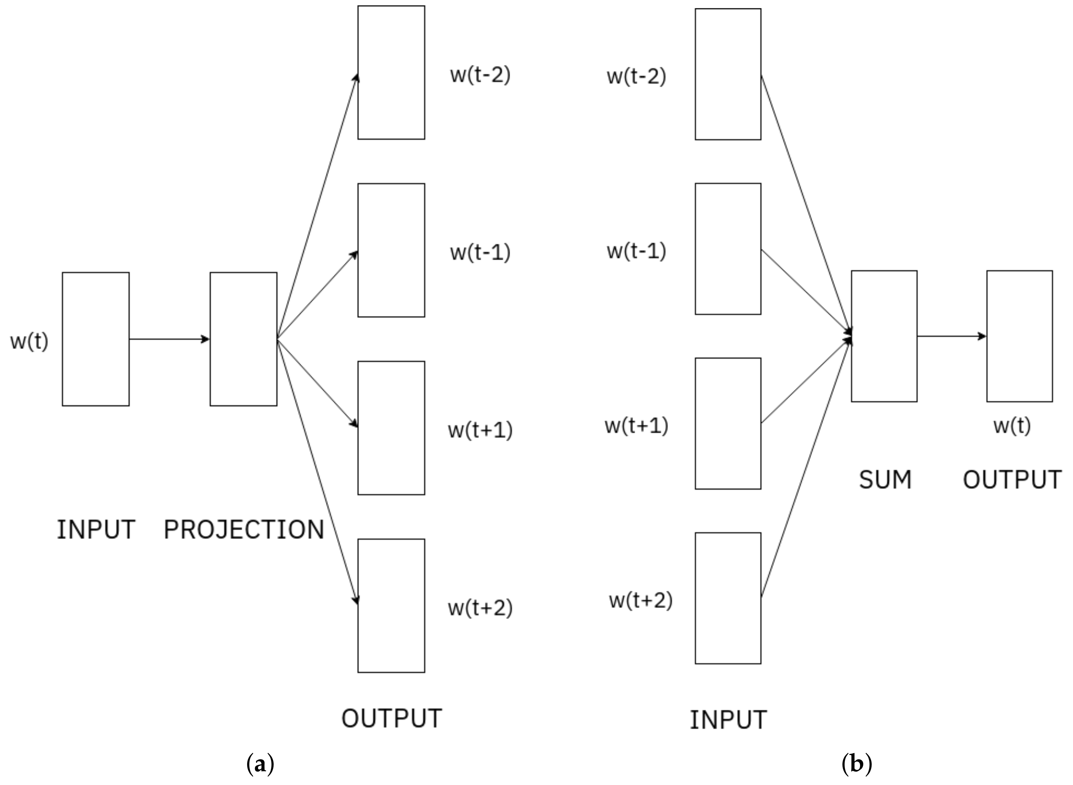
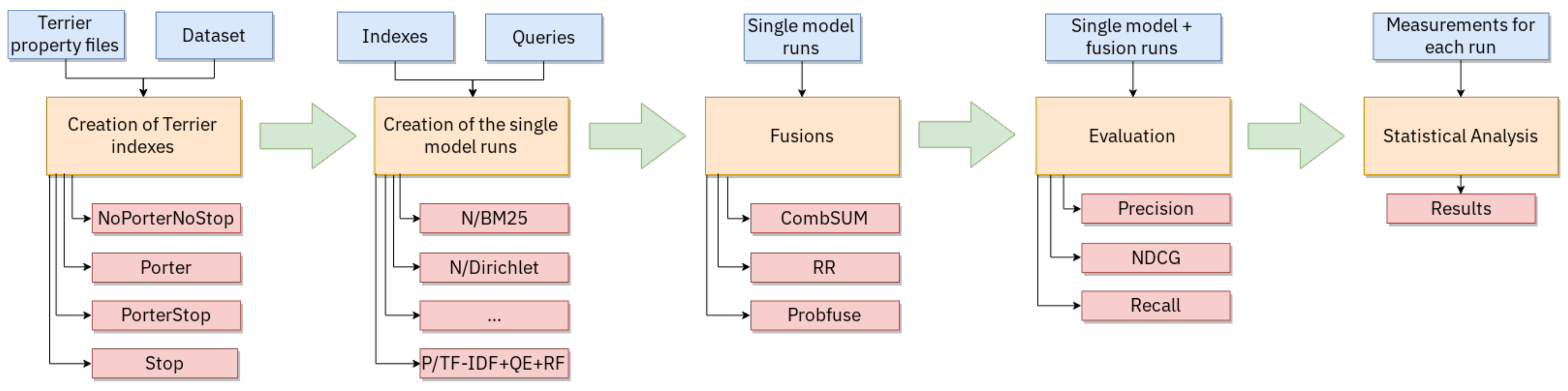
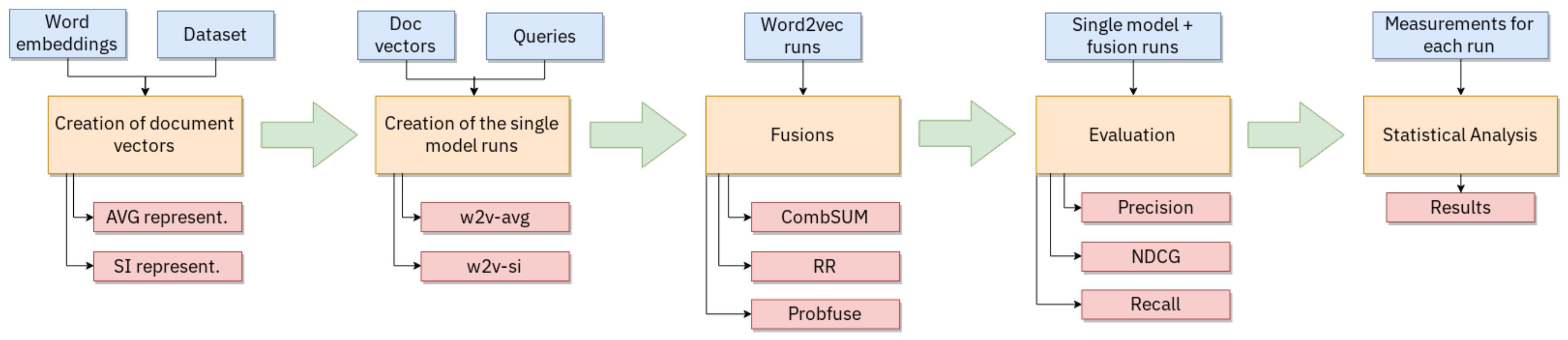
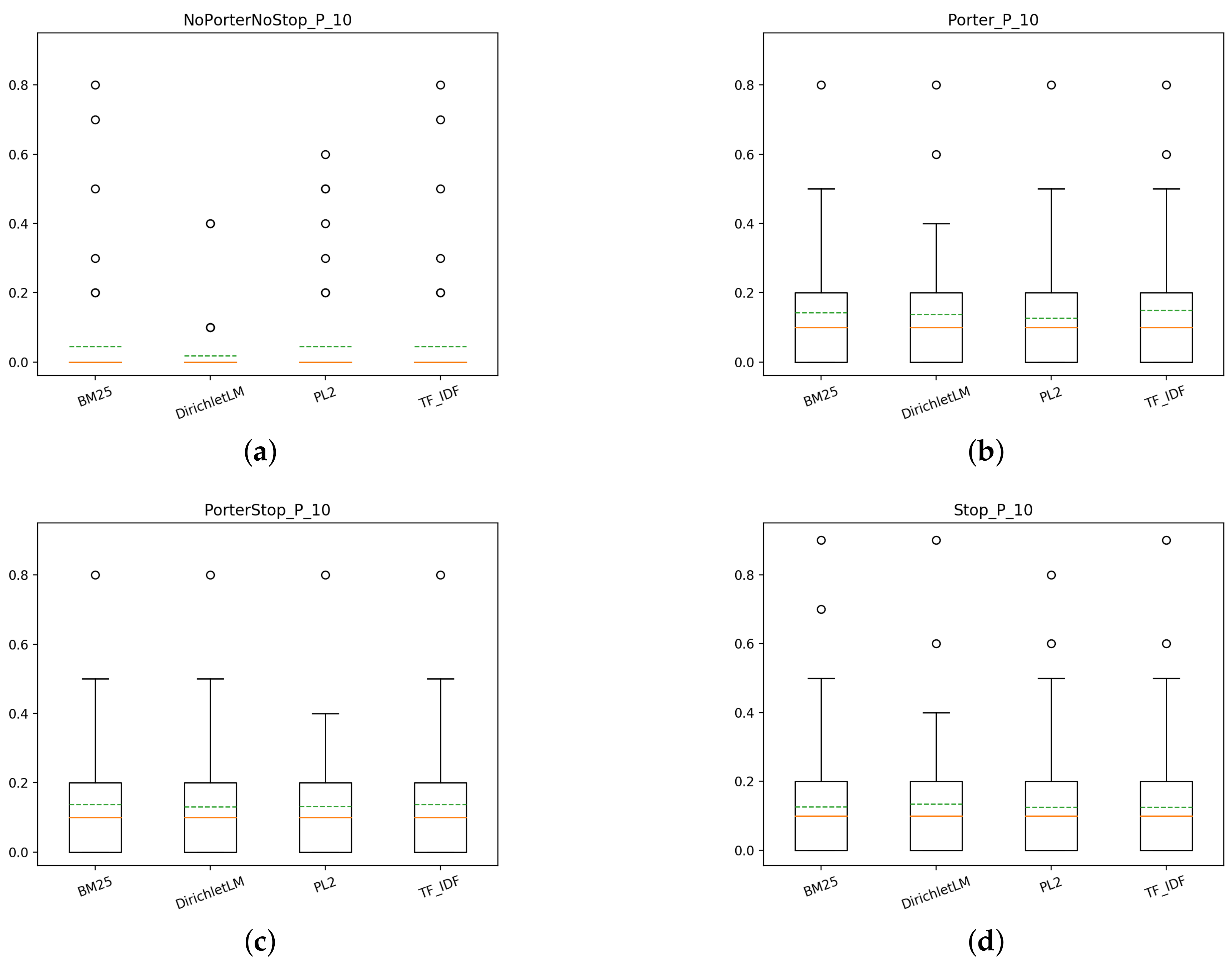
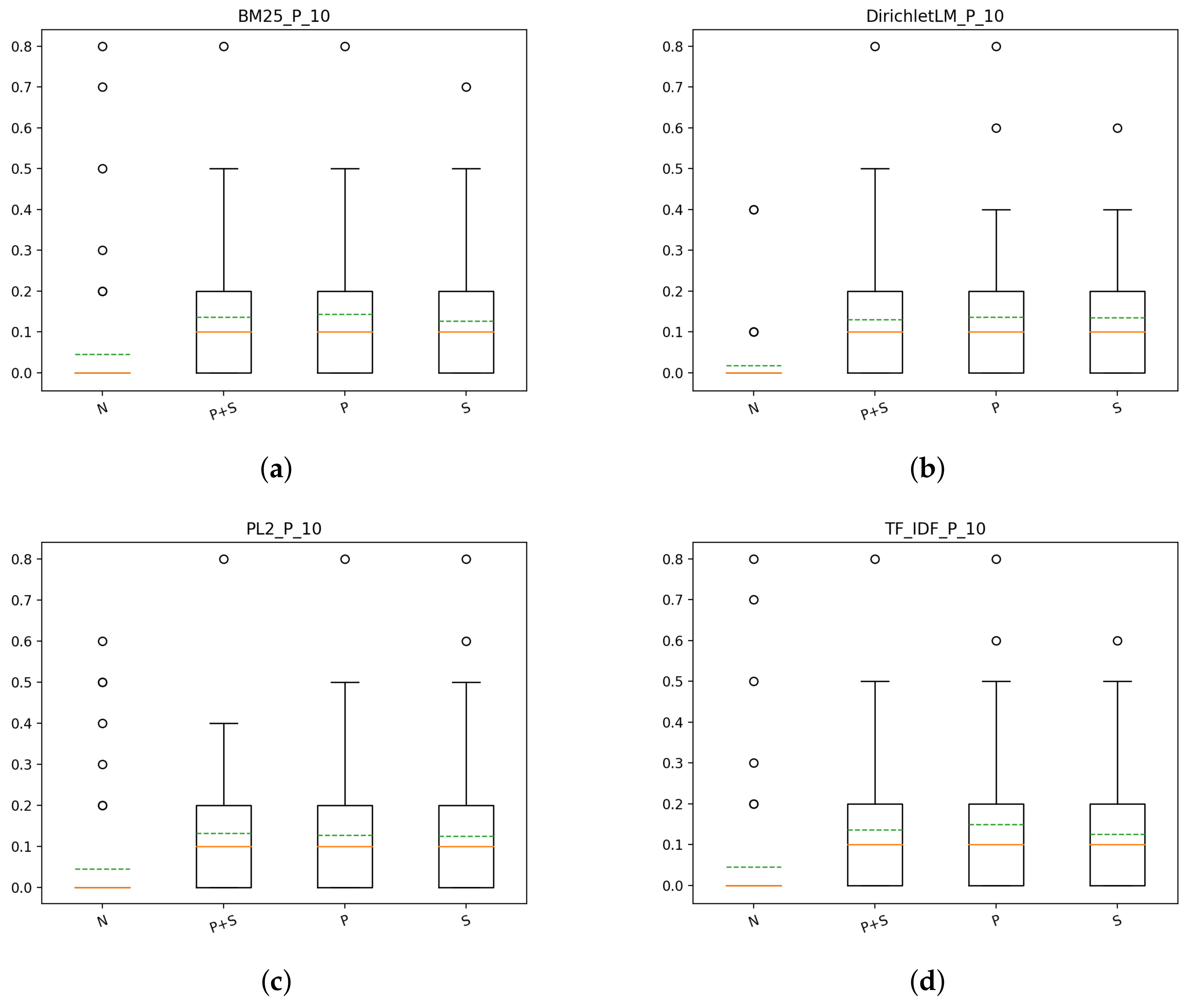
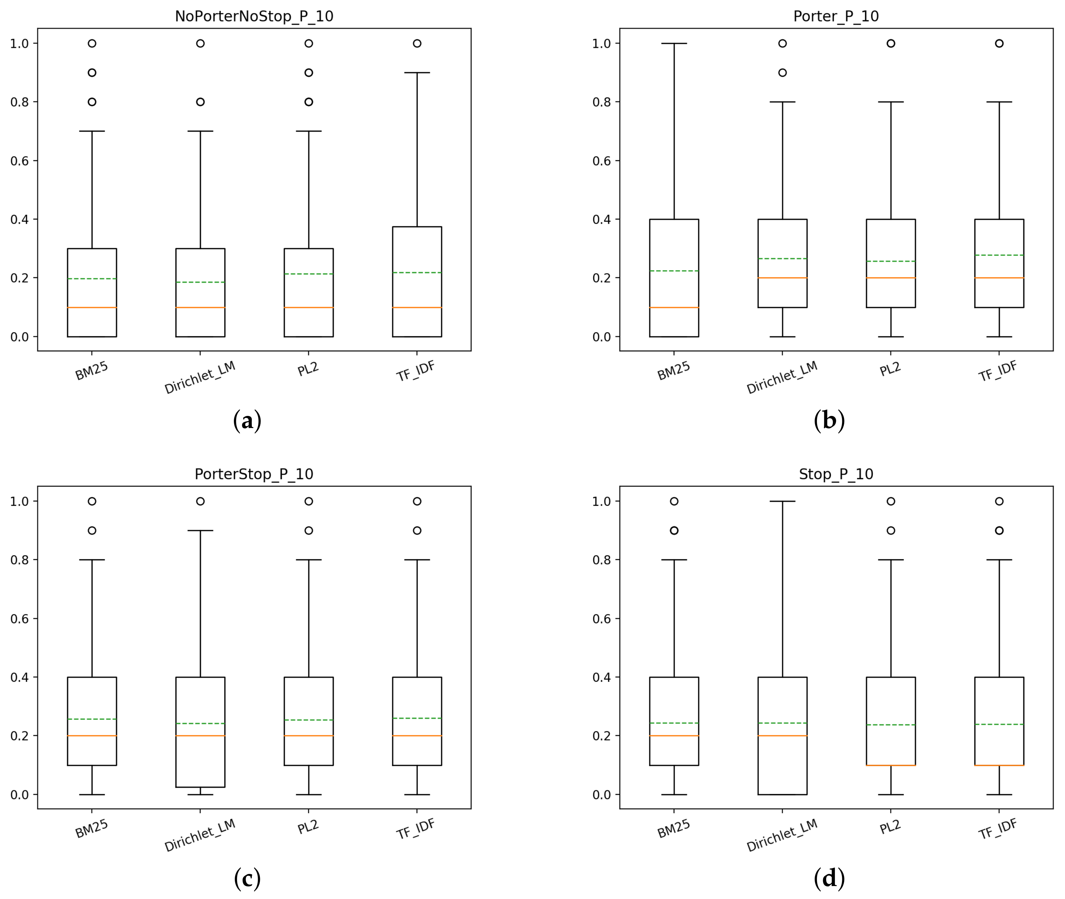
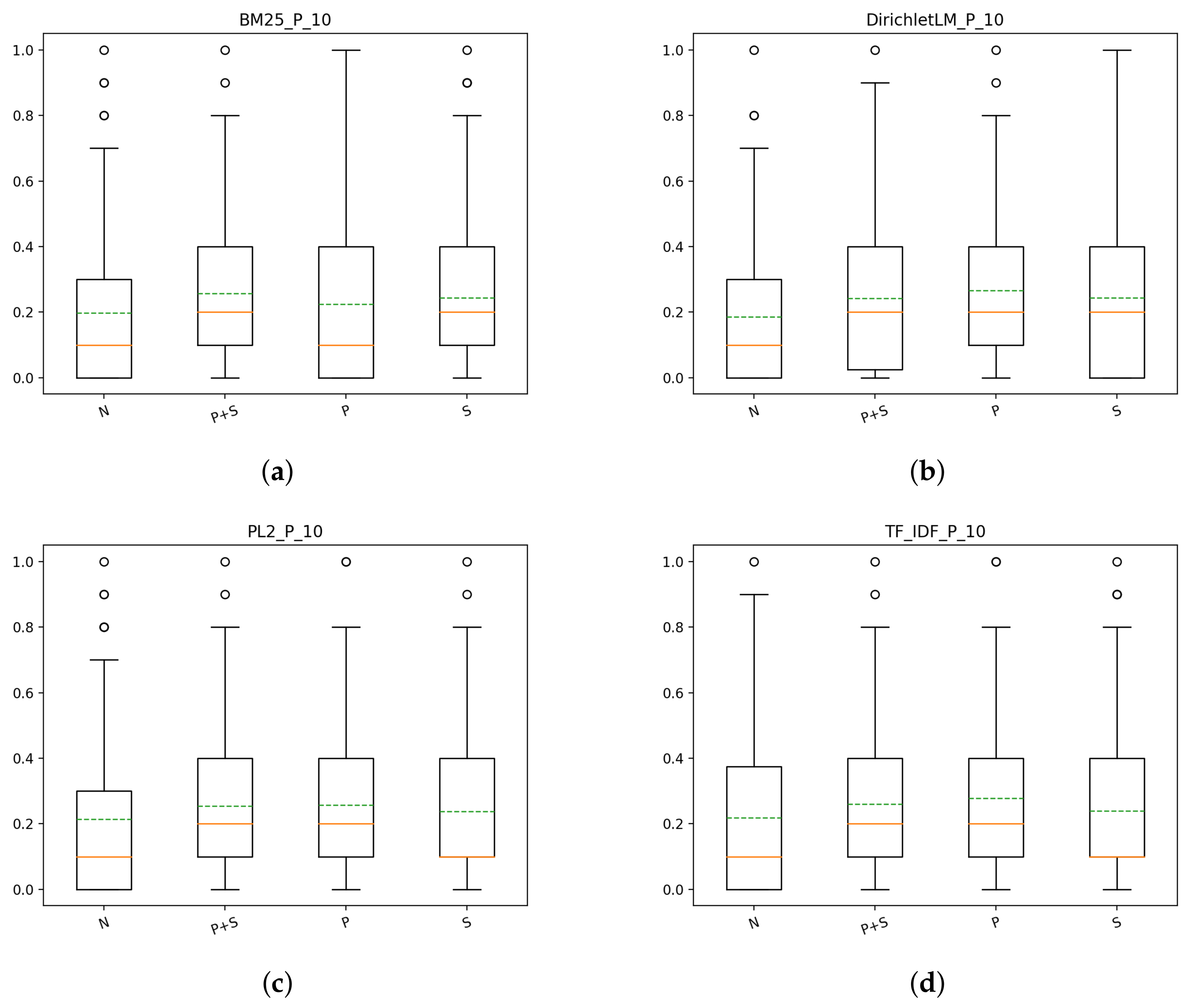
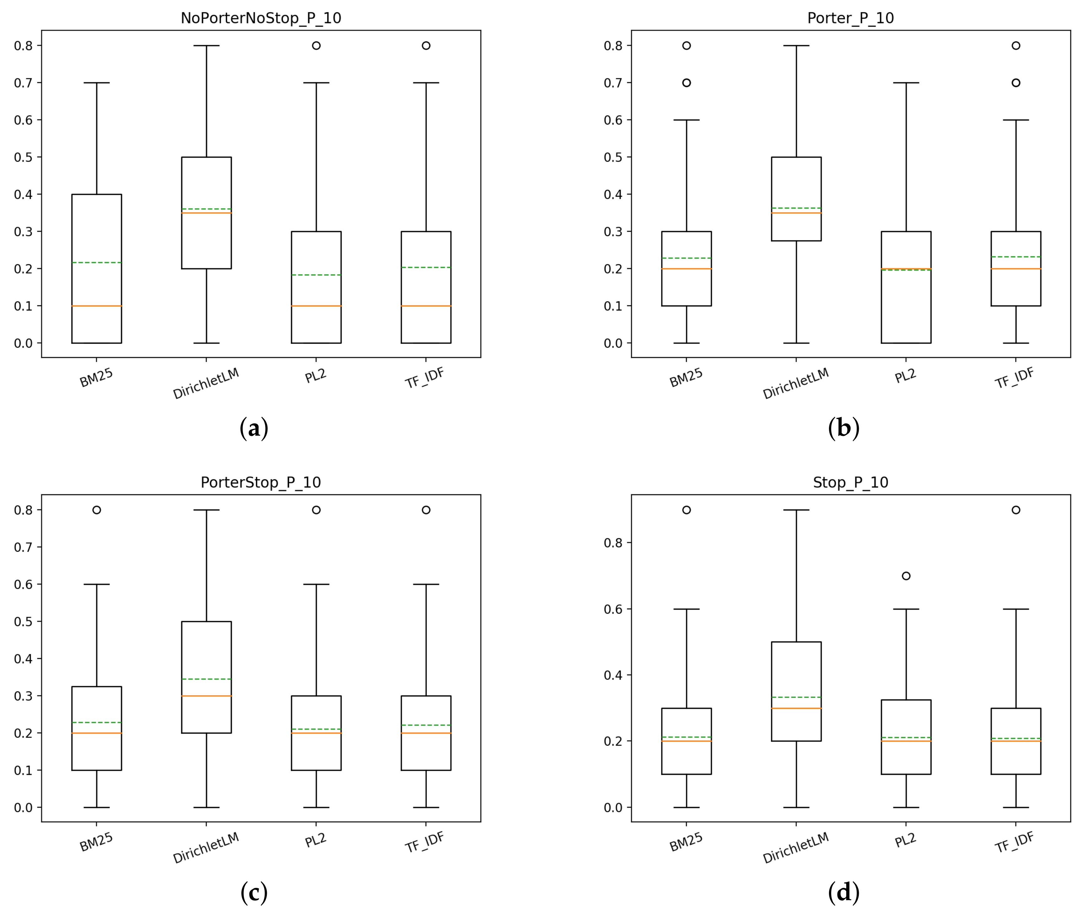
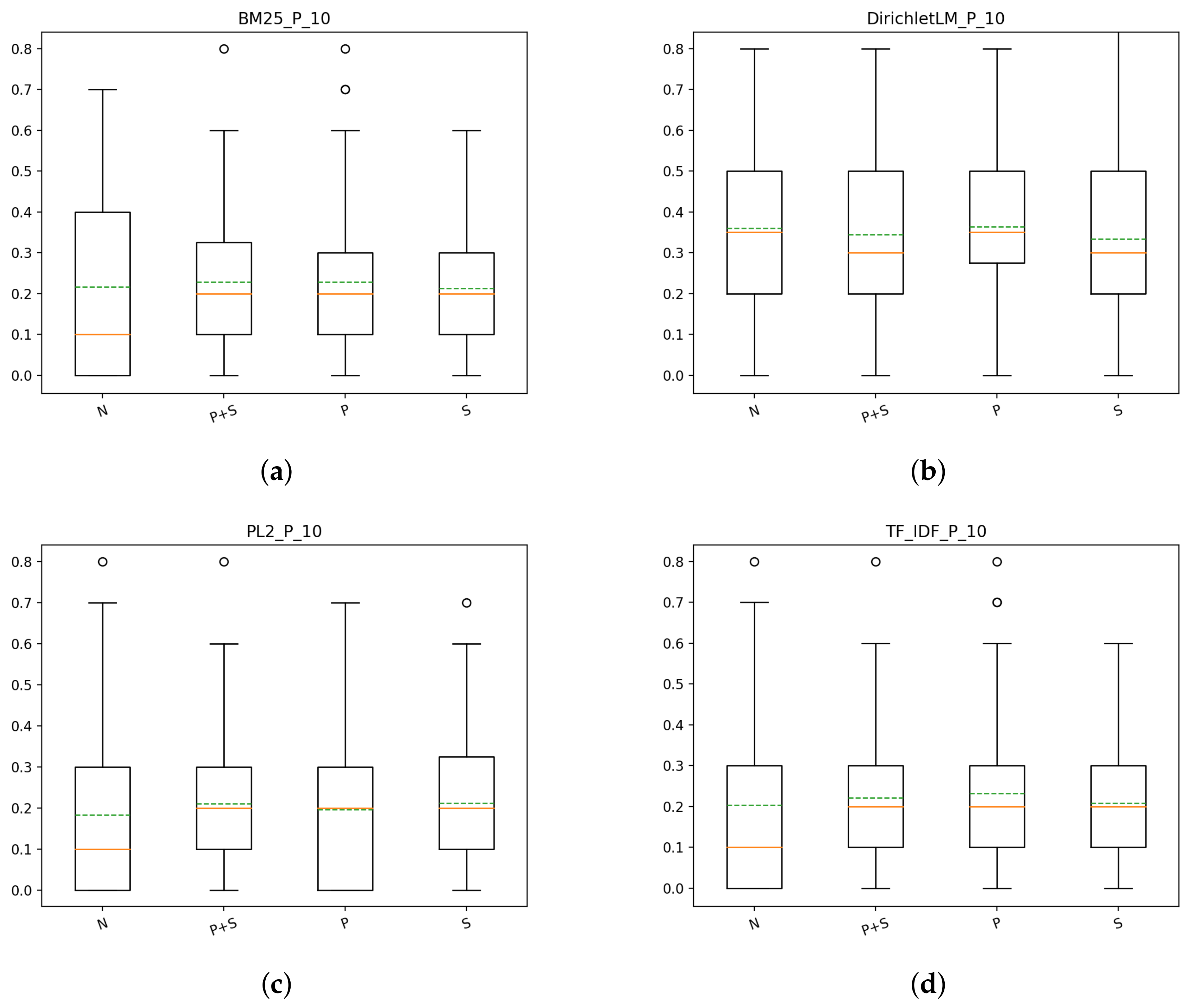
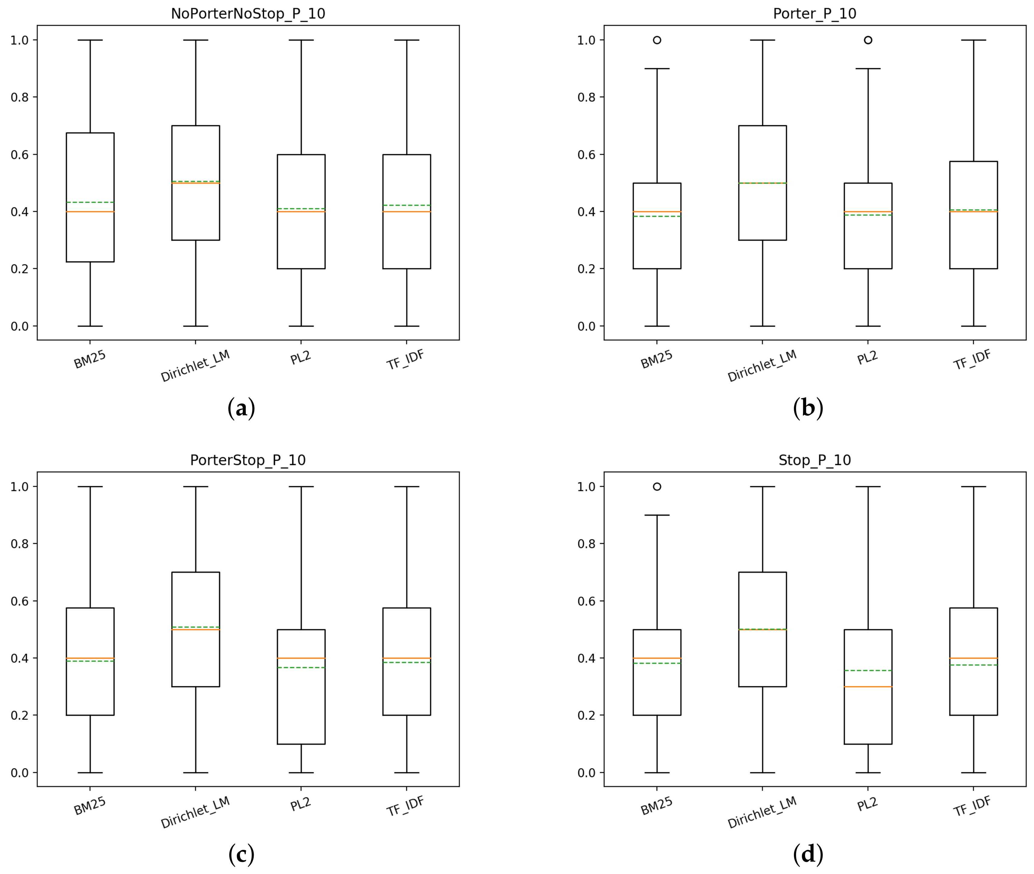
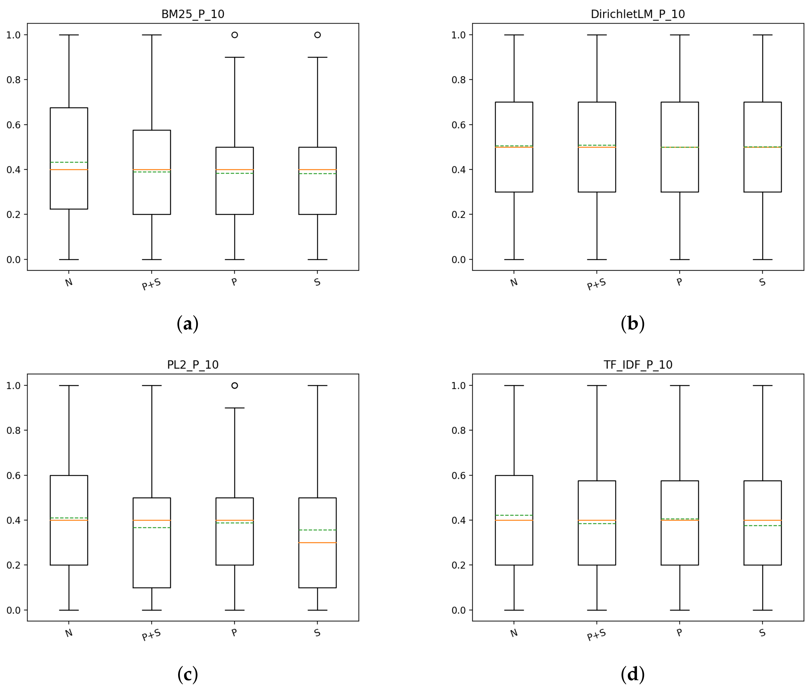
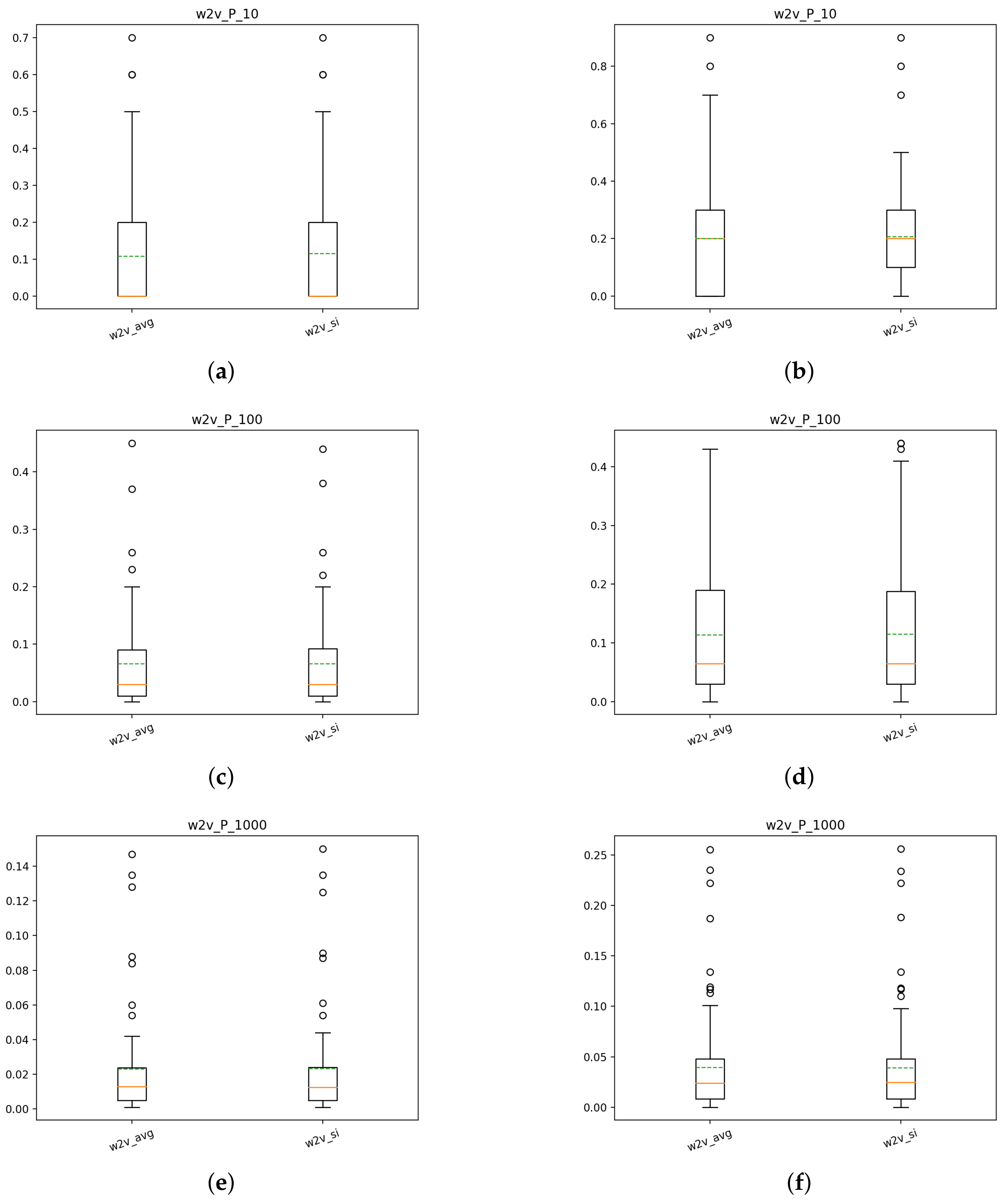
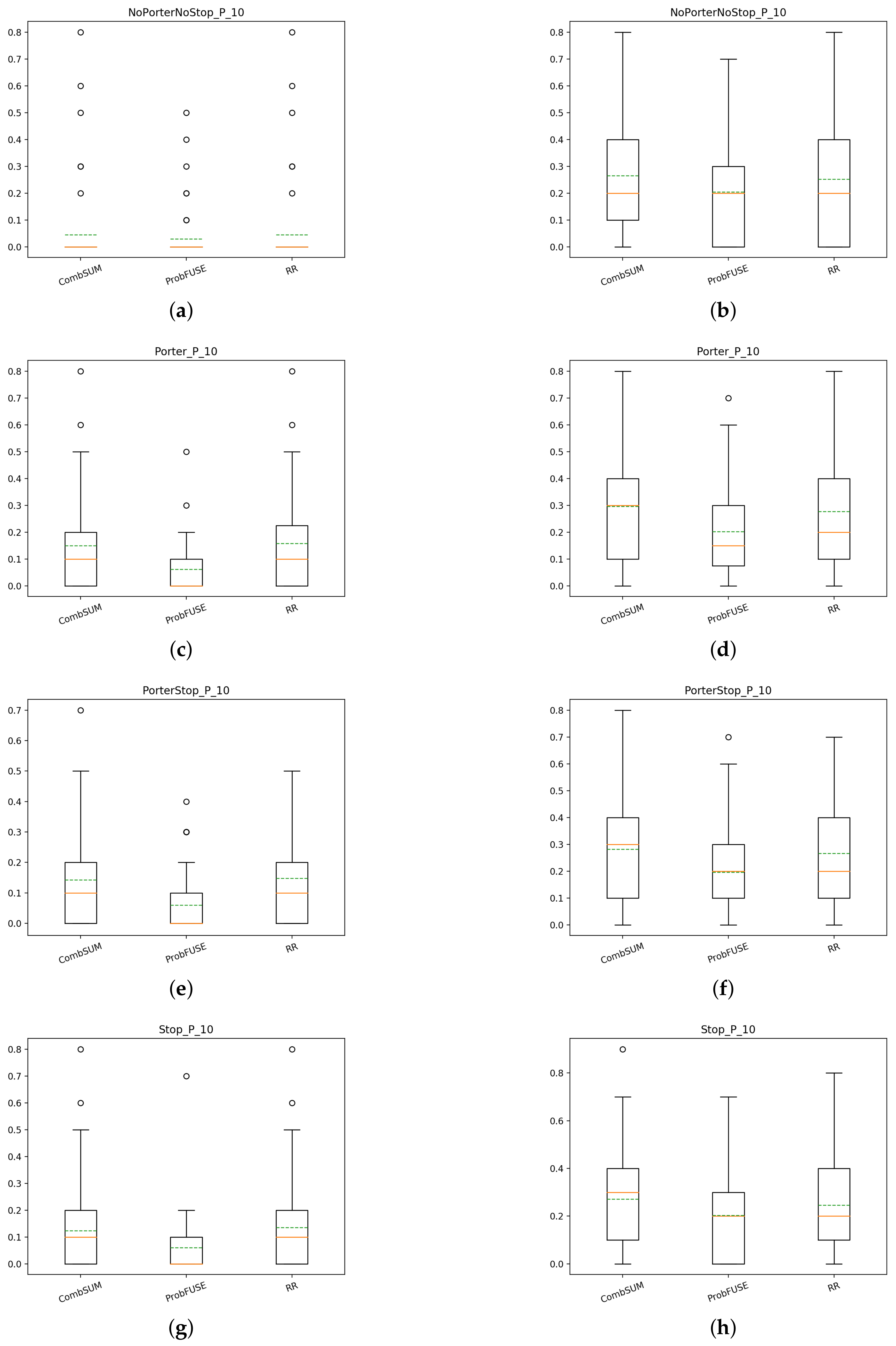
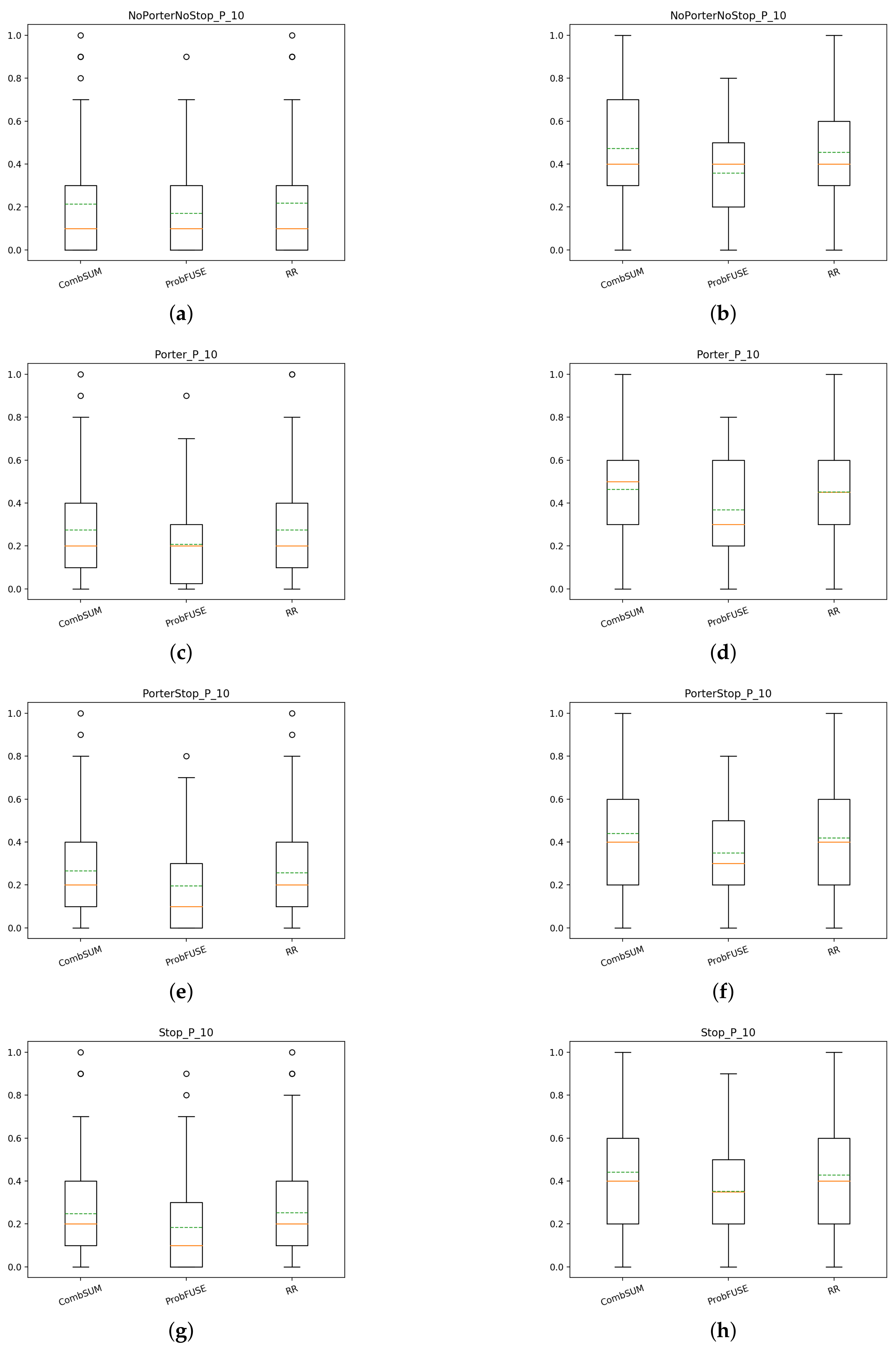
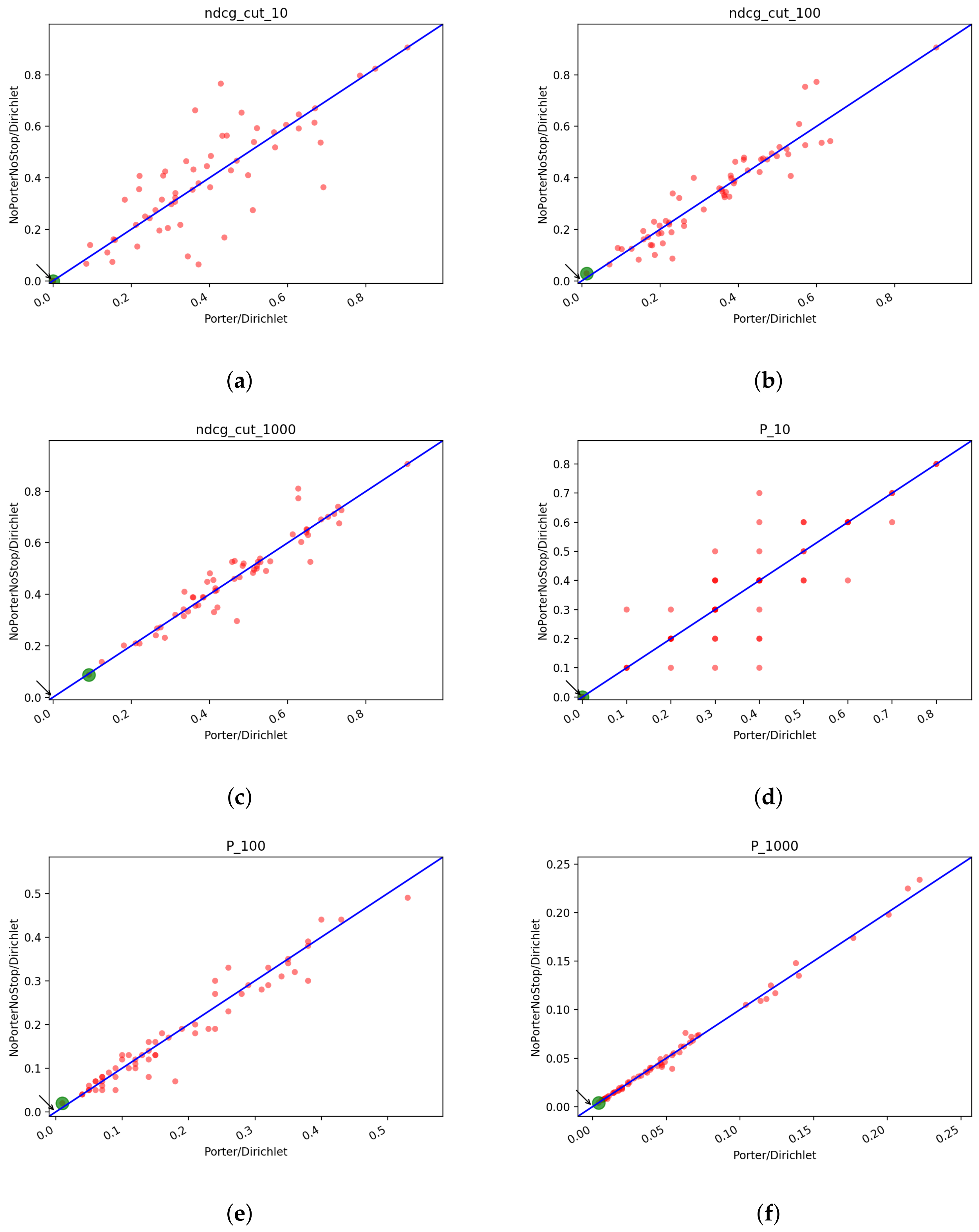
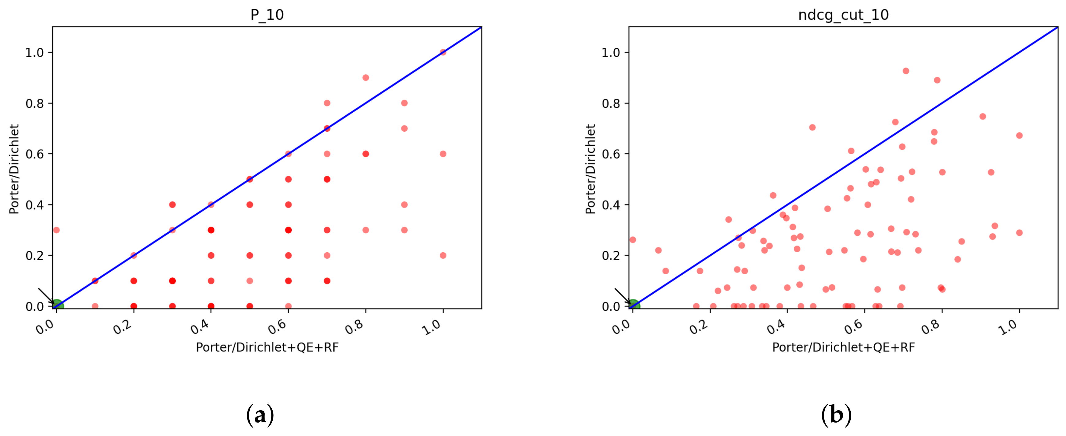
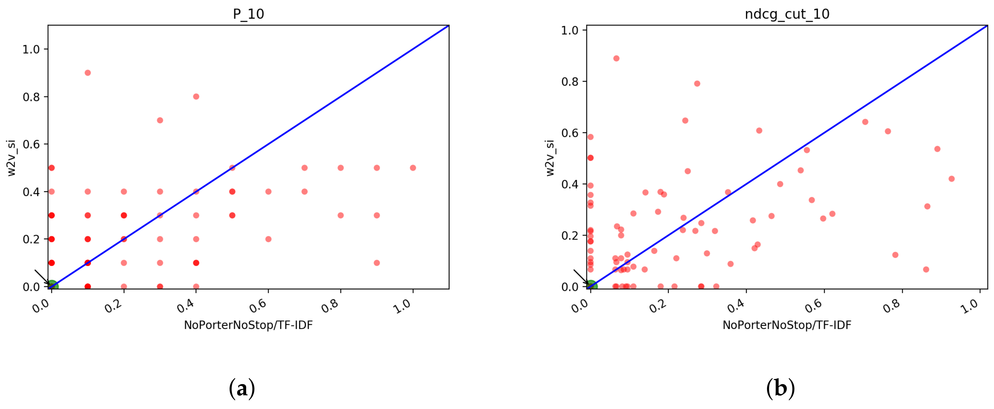
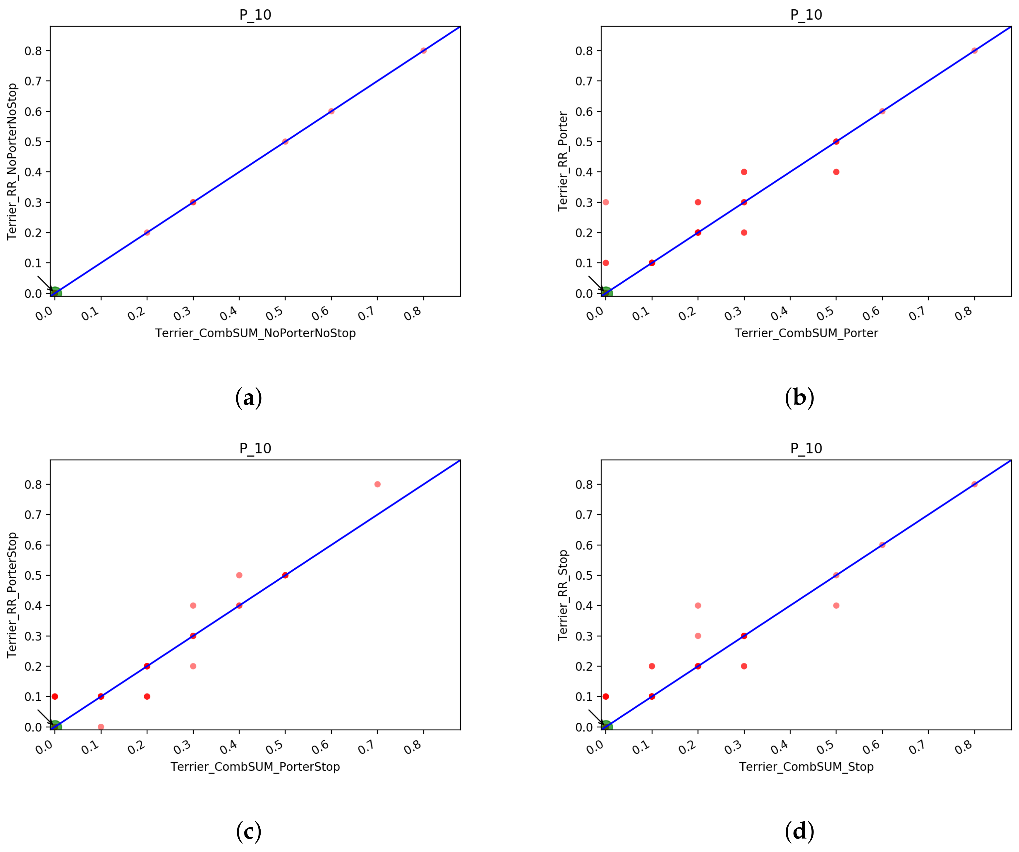
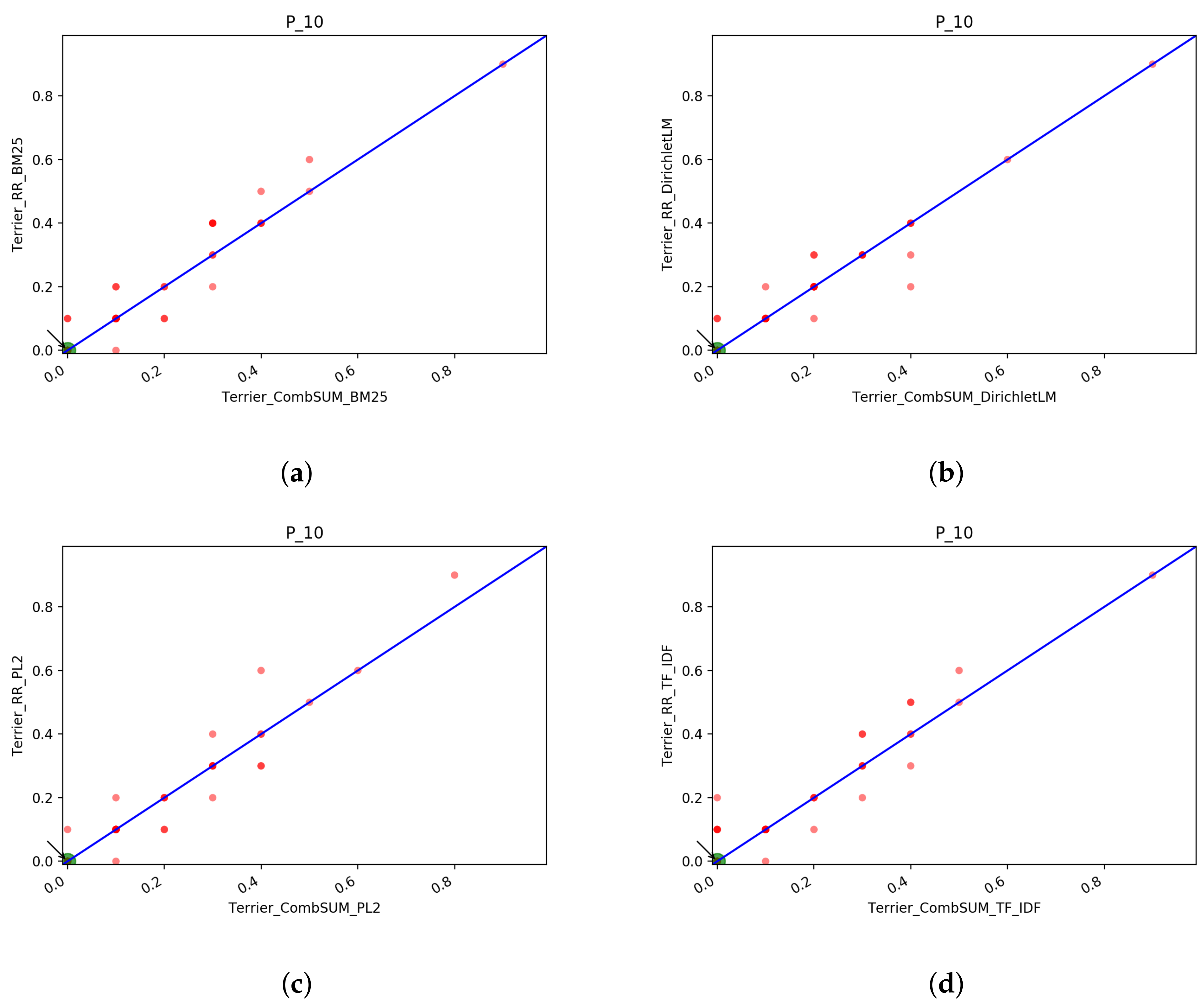
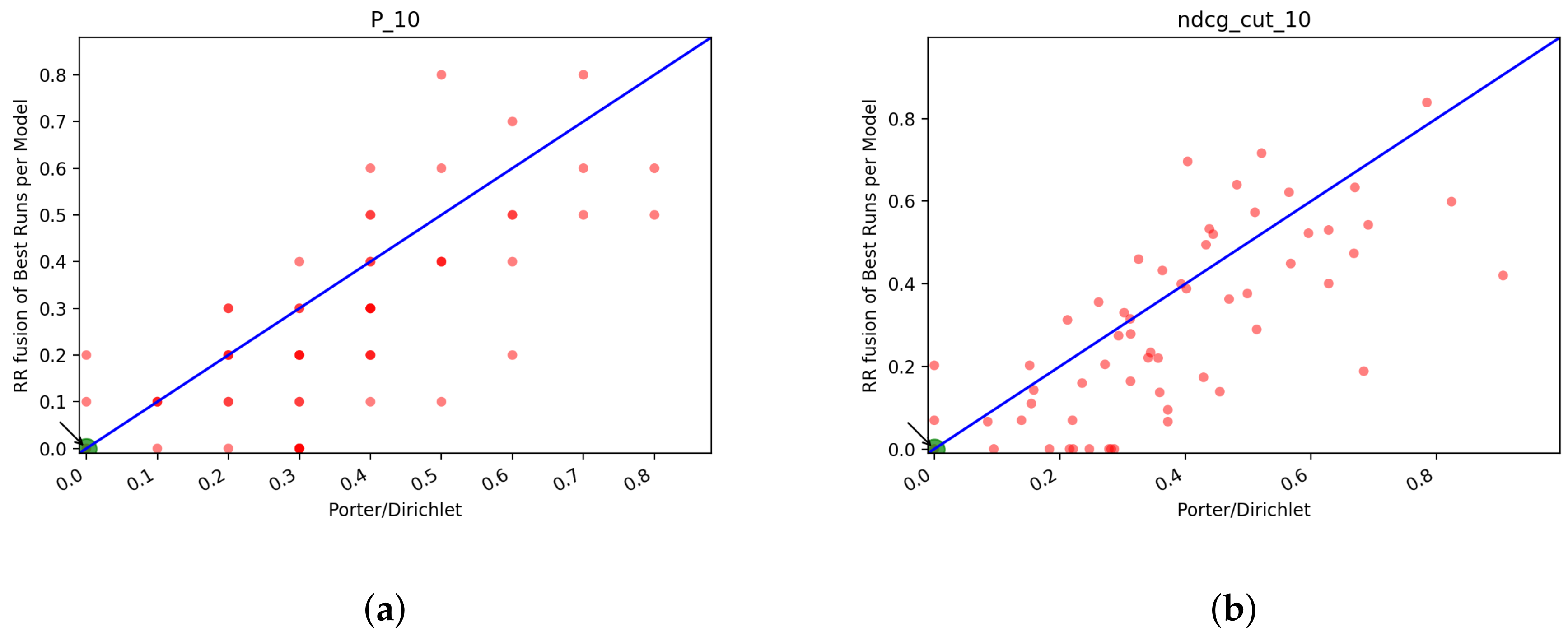
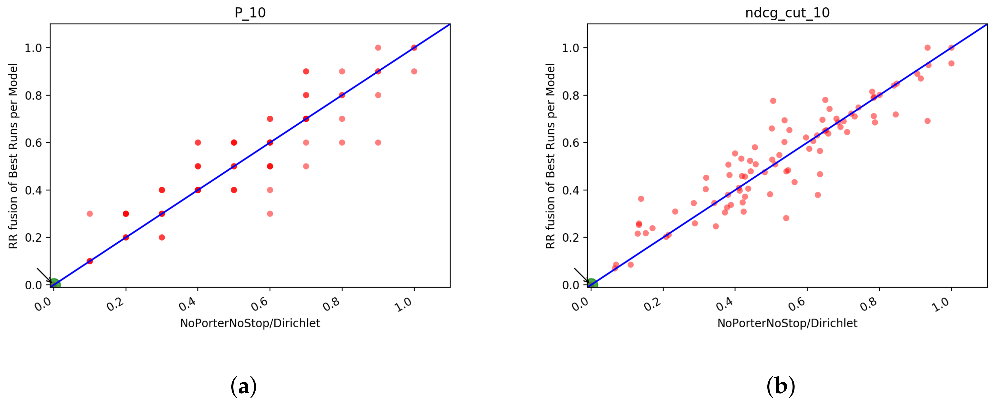
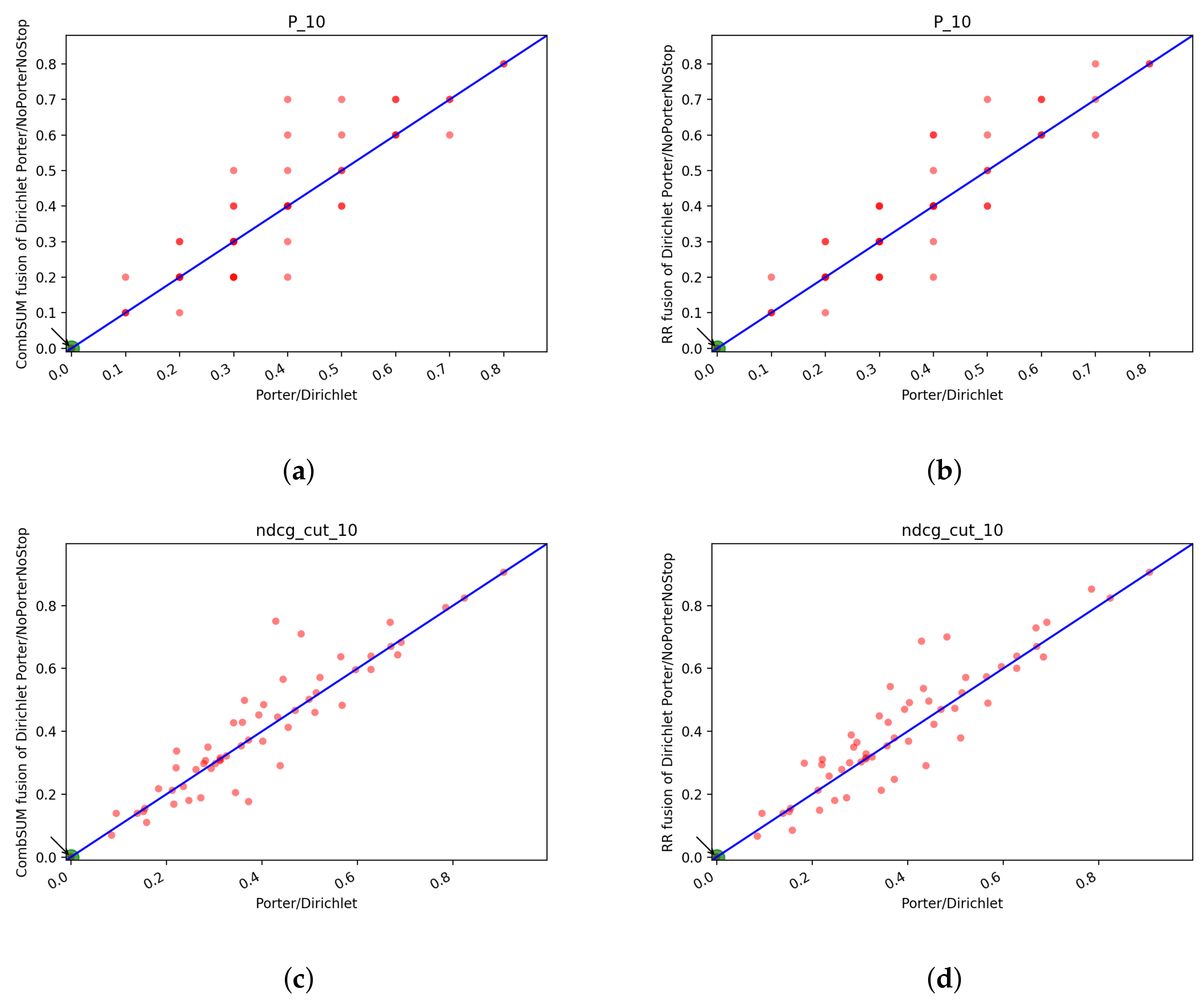
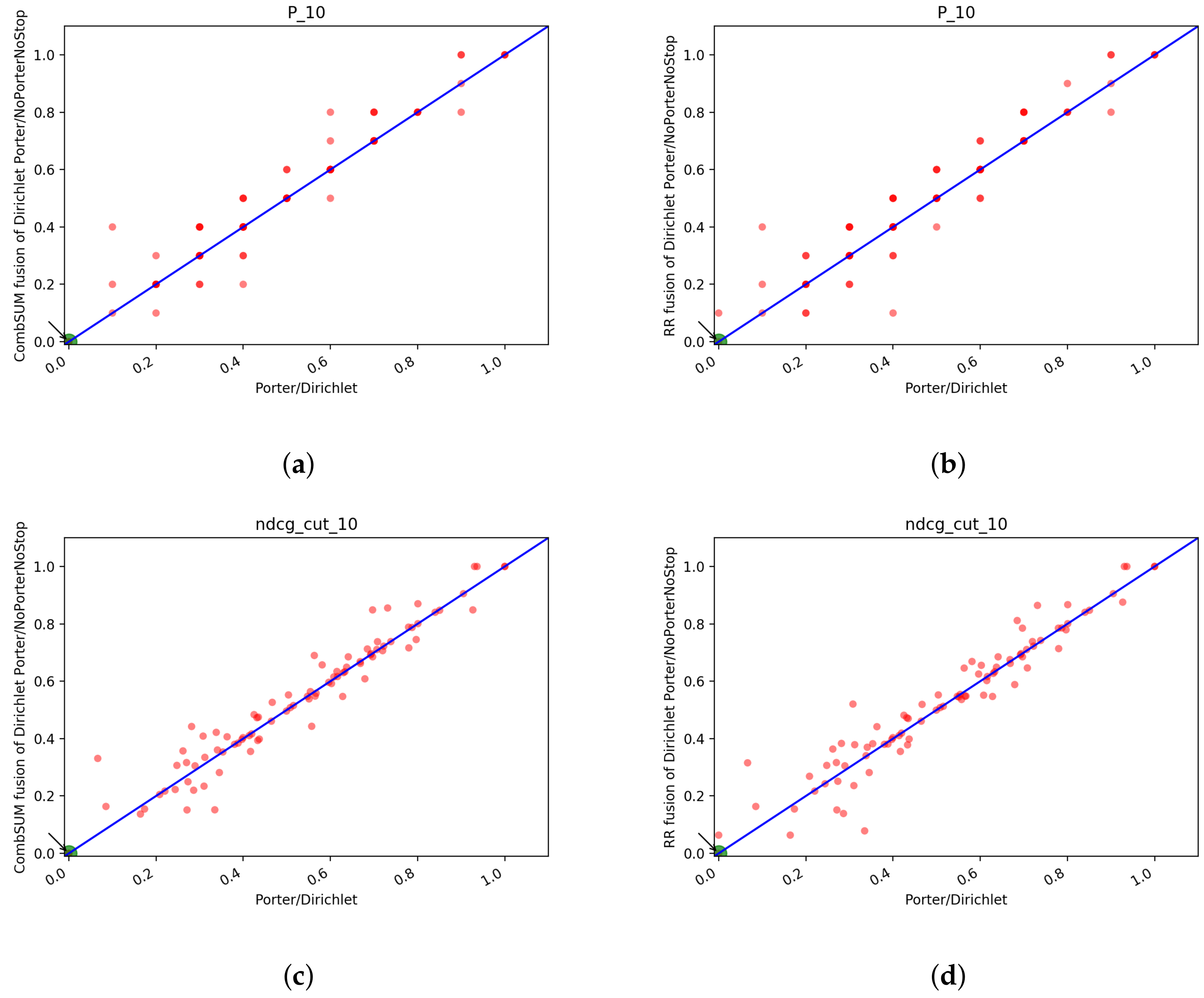
Table 1.
Summary of the datasets used.
| Task | Tracks | Dataset | # Topics |
|---|---|---|---|
| T1 | 2018, 2019 | All articles of PUBMED | 60 |
| T2 | 2017, 2018, 2019 | Result of boolean search on PUBMED | 90 |
Table 2.
Summary of all the runs analyzed per research question.
| RQ | Runs | Total per Task |
|---|---|---|
| RQ1 | BM25, Dirichlet, PL2, TF-IDF, w2v-avg, w2v-si | 18 |
| RQ2 | QE+RF of BM25, Dirichlet, PL2, TF-IDF | 16 |
| RQ3 | RQ1, RQ2, N, P, P+S, S | 18 |
Table 3.
NDCG at various cut offs and Recall@R for the different models for T1. The highest values are in bold.
Table 3.
NDCG at various cut offs and Recall@R for the different models for T1. The highest values are in bold.
| Index/Model | NDCG@10 | NDCG@100 | NDCG@1000 | R@R |
|---|---|---|---|---|
| NoPorterNoStop/BM25 | 0.0443 | 0.0389 | 0.082 | 0.0244 |
| NoPorterNoStop/Dirichlet | 0.0167 | 0.0238 | 0.065 | 0.0169 |
| NoPorterNoStop/PL2 | 0.0454 | 0.0387 | 0.0782 | 0.0243 |
| NoPorterNoStop/TF_IDF | 0.0448 | 0.0393 | 0.0821 | 0.0248 |
| Porter/BM25 | 0.1346 | 0.1538 | 0.2549 | 0.1045 |
| Porter/Dirichlet | 0.1276 | 0.1652 | 0.2749 | 0.1088 |
| Porter/PL2 | 0.1257 | 0.1495 | 0.2462 | 0.0985 |
| Porter/TF_IDF | 0.1451 | 0.1682 | 0.2692 | 0.1077 |
| PorterStop/BM25 | 0.1316 | 0.1559 | 0.2597 | 0.1004 |
| PorterStop/Dirichlet | 0.1217 | 0.1612 | 0.2662 | 0.1003 |
| PorterStop/PL2 | 0.1297 | 0.1461 | 0.2426 | 0.0928 |
| PorterStop/TF_IDF | 0.1306 | 0.1551 | 0.258 | 0.1001 |
| Stop/BM25 | 0.1186 | 0.1458 | 0.2374 | 0.0911 |
| Stop/Dirichlet | 0.1243 | 0.1538 | 0.2496 | 0.1017 |
| Stop/PL2 | 0.1209 | 0.1396 | 0.2238 | 0.0851 |
| Stop/TF_IDF | 0.1172 | 0.1464 | 0.237 | 0.0911 |
Table 4.
NDCG at various cut offs and Recall@R for the different models for T2. The highest values are in bold.
Table 4.
NDCG at various cut offs and Recall@R for the different models for T2. The highest values are in bold.
| Index/Model | NDCG@10 | NDCG@100 | NDCG@1000 | R@R |
|---|---|---|---|---|
| NoPorterNoStop/BM25 | 0.1861 | 0.2406 | 0.3737 | 0.166 |
| NoPorterNoStop/Dirichlet | 0.1786 | 0.2526 | 0.3878 | 0.1707 |
| NoPorterNoStop/PL2 | 0.2052 | 0.2525 | 0.3929 | 0.1803 |
| NoPorterNoStop/TF_IDF | 0.2075 | 0.2665 | 0.4031 | 0.1835 |
| Porter/BM25 | 0.2162 | 0.2654 | 0.4127 | 0.1814 |
| Porter/Dirichlet | 0.2662 | 0.3165 | 0.459 | 0.2067 |
| Porter/PL2 | 0.2565 | 0.2969 | 0.4464 | 0.2041 |
| Porter/TF_IDF | 0.2761 | 0.3202 | 0.4716 | 0.2156 |
| PorterStop/BM25 | 0.26 | 0.3144 | 0.4682 | 0.2062 |
| PorterStop/Dirichlet | 0.2438 | 0.3032 | 0.4456 | 0.1959 |
| PorterStop/PL2 | 0.2584 | 0.3058 | 0.4608 | 0.2037 |
| PorterStop/TF_IDF | 0.2618 | 0.3148 | 0.4683 | 0.2072 |
| Stop/BM25 | 0.2396 | 0.2967 | 0.4501 | 0.2004 |
| Stop/Dirichlet | 0.2363 | 0.2977 | 0.4373 | 0.1981 |
| Stop/PL2 | 0.2387 | 0.2933 | 0.4455 | 0.196 |
| Stop/TF_IDF | 0.2391 | 0.2987 | 0.451 | 0.2015 |
Table 5.
T1: NDCG at various cut offs and Recall@R for the different models with QE+RF. The highest values are in bold.
Table 5.
T1: NDCG at various cut offs and Recall@R for the different models with QE+RF. The highest values are in bold.
| Index/Model | NDCG@10 | NDCG@100 | NDCG@1000 | R@R |
|---|---|---|---|---|
| NoPorterNoStop/BM25 | 0.2313 | 0.227 | 0.3382 | 0.1471 |
| NoPorterNoStop/Dirichlet | 0.3792 | 0.339 | 0.4687 | 0.2332 |
| NoPorterNoStop/PL2 | 0.1987 | 0.2003 | 0.3101 | 0.1282 |
| NoPorterNoStop/TF_IDF | 0.2162 | 0.2182 | 0.3297 | 0.1385 |
| Porter/BM25 | 0.2417 | 0.2603 | 0.3872 | 0.1728 |
| Porter/Dirichlet | 0.3778 | 0.3397 | 0.4684 | 0.2329 |
| Porter/PL2 | 0.2114 | 0.2433 | 0.372 | 0.1549 |
| Porter/TF_IDF | 0.2404 | 0.2576 | 0.3855 | 0.1624 |
| PorterStop/BM25 | 0.2397 | 0.2484 | 0.3763 | 0.1584 |
| PorterStop/Dirichlet | 0.3498 | 0.3256 | 0.4558 | 0.2252 |
| PorterStop/PL2 | 0.2237 | 0.2337 | 0.3609 | 0.1485 |
| PorterStop/TF_IDF | 0.233 | 0.2453 | 0.3736 | 0.1571 |
| Stop/BM25 | 0.2201 | 0.239 | 0.3619 | 0.1586 |
| Stop/Dirichlet | 0.3436 | 0.3273 | 0.4551 | 0.2372 |
| Stop/PL2 | 0.2112 | 0.2234 | 0.3443 | 0.1503 |
| Stop/TF_IDF | 0.2139 | 0.2354 | 0.3575 | 0.1573 |
Table 6.
DirichletLM+QE+RF for T1: P@10, P@100 and P@1000. The highest values are in bold.
| Index | P@10 | P@100 | P@1000 |
|---|---|---|---|
| NoPorterNoStop | 0.36 | 0.1782 | 0.0557 |
| Porter | 0.3633 | 0.1842 | 0.0558 |
| PorterStop | 0.345 | 0.1773 | 0.0549 |
| Stop | 0.3333 | 0.1853 | 0.0553 |
Table 7.
T2: NDCG at various cut offs and Recall@R for the different models with QE+RF. The highest values are in bold.
Table 7.
T2: NDCG at various cut offs and Recall@R for the different models with QE+RF. The highest values are in bold.
| Index/Model | NDCG@10 | NDCG@100 | NDCG@1000 | R@R |
|---|---|---|---|---|
| NoPorterNoStop/BM25 | 0.4449 | 0.474 | 0.6113 | 0.3321 |
| NoPorterNoStop/Dirichlet | 0.5231 | 0.5359 | 0.6644 | 0.3857 |
| NoPorterNoStop/PL2 | 0.42 | 0.4581 | 0.6019 | 0.3239 |
| NoPorterNoStop/TF_IDF | 0.4325 | 0.4681 | 0.6092 | 0.3175 |
| Porter/BM25 | 0.3966 | 0.434 | 0.5815 | 0.3007 |
| Porter/Dirichlet | 0.5213 | 0.5367 | 0.6648 | 0.3877 |
| Porter/PL2 | 0.3939 | 0.4398 | 0.5878 | 0.3097 |
| Porter/TF_IDF | 0.4182 | 0.4557 | 0.603 | 0.3125 |
| PorterStop/BM25 | 0.4045 | 0.4484 | 0.5981 | 0.3066 |
| PorterStop/Dirichlet | 0.52 | 0.5231 | 0.6525 | 0.3741 |
| PorterStop/PL2 | 0.3801 | 0.4356 | 0.5864 | 0.3013 |
| PorterStop/TF_IDF | 0.3958 | 0.443 | 0.5931 | 0.3017 |
| Stop/BM25 | 0.3868 | 0.4329 | 0.5829 | 0.3046 |
| Stop/Dirichlet | 0.5149 | 0.5231 | 0.6544 | 0.3691 |
| Stop/PL2 | 0.3616 | 0.4225 | 0.574 | 0.2955 |
| Stop/TF_IDF | 0.3776 | 0.4272 | 0.5781 | 0.2985 |
Table 8.
DirichletLM+QE+RF for T2: P@10, P@100 and P@1000. The highest values are in bold.
| Index | P@10 | P@100 | P@1000 |
|---|---|---|---|
| NoPorterNoStop | 0.5056 | 0.2412 | 0.0602 |
| Porter | 0.5 | 0.2412 | 0.0601 |
| PorterStop | 0.5089 | 0.2337 | 0.0593 |
| Stop | 0.5011 | 0.2351 | 0.0599 |
Table 9.
T1: scores of NDCG and R@R of w2v runs and Terrier with NoPorterNoStop index.
| Index/Model | NDCG@10 | NDCG@100 | NDCG@1000 | R@R |
|---|---|---|---|---|
| w2v_avg | 0.1144 | 0.1109 | 0.1692 | 0.0689 |
| w2v_si | 0.1185 | 0.1123 | 0.1708 | 0.0688 |
| NoPorterNoStop/BM25 | 0.0443 | 0.0389 | 0.082 | 0.0244 |
| NoPorterNoStop/Dirichlet | 0.0167 | 0.0238 | 0.065 | 0.0169 |
| NoPorterNoStop/PL2 | 0.0454 | 0.0387 | 0.0782 | 0.0243 |
| NoPorterNoStop/TF_IDF | 0.0448 | 0.0393 | 0.0821 | 0.0248 |
Table 10.
T2: scores of NDCG and R@R of w2v runs and Terrier with NoPorterNoStop index.
| Index/Model | NDCG@10 | NDCG@100 | NDCG@1000 | R@R |
|---|---|---|---|---|
| w2v_avg | 0.2065 | 0.2228 | 0.3523 | 0.1328 |
| w2v_si | 0.2104 | 0.2238 | 0.3539 | 0.1347 |
| NoPorterNoStop/BM25 | 0.1861 | 0.2406 | 0.3737 | 0.166 |
| NoPorterNoStop/Dirichlet | 0.1786 | 0.2526 | 0.3878 | 0.1707 |
| NoPorterNoStop/PL2 | 0.2052 | 0.2525 | 0.3929 | 0.1803 |
| NoPorterNoStop/TF_IDF | 0.2075 | 0.2665 | 0.4031 | 0.1835 |
Table 11.
T1: NDCG and Recall@R for the fusion runs. The highest values are in bold.
| Index/Fusion | NDCG@10 | NDCG@100 | NDCG@1000 | R@R |
|---|---|---|---|---|
| N/CombSUM | 0.0474 | 0.0439 | 0.0836 | 0.0246 |
| N/ProbFUSE | 0.0269 | 0.0378 | 0.0778 | 0.0249 |
| N/RR | 0.0453 | 0.0405 | 0.0794 | 0.0241 |
| P/CombSUM | 0.1438 | 0.1715 | 0.2718 | 0.1095 |
| P/ProbFUSE | 0.0552 | 0.1498 | 0.2569 | 0.1013 |
| P/RR | 0.1538 | 0.1701 | 0.2726 | 0.1096 |
| P+S/CombSUM | 0.1383 | 0.1628 | 0.2671 | 0.105 |
| P+S/ProbFUSE | 0.0543 | 0.1441 | 0.2499 | 0.0932 |
| P+S/RR | 0.1447 | 0.1635 | 0.2649 | 0.1029 |
| S/CombSUM | 0.1198 | 0.1551 | 0.242 | 0.0973 |
| S/ProbFUSE | 0.0634 | 0.1427 | 0.2368 | 0.0875 |
| S/RR | 0.1264 | 0.1529 | 0.2437 | 0.0973 |
Table 12.
T1: NDCG and Recall@R for the fusion runs with QE+RF. The highest values are in bold.
| Index/Fusion | NDCG@10 | NDCG@100 | NDCG@1000 | R@R |
|---|---|---|---|---|
| N/CombSUM | 0.2861 | 0.2756 | 0.3749 | 0.1813 |
| N/ProbFUSE | 0.1995 | 0.2476 | 0.3918 | 0.1702 |
| N/RR | 0.2796 | 0.2588 | 0.3984 | 0.1672 |
| P/CombSUM | 0.3084 | 0.3154 | 0.4278 | 0.2101 |
| P/ProbFUSE | 0.1798 | 0.269 | 0.4107 | 0.1912 |
| P/RR | 0.2952 | 0.2964 | 0.4341 | 0.1942 |
| P+S/CombSUM | 0.2889 | 0.2963 | 0.4135 | 0.1963 |
| P+S/ProbFUSE | 0.1758 | 0.2499 | 0.3975 | 0.1788 |
| P+S/RR | 0.2878 | 0.2801 | 0.4224 | 0.1822 |
| S/CombSUM | 0.2824 | 0.2842 | 0.3956 | 0.1915 |
| S/ProbFUSE | 0.1874 | 0.248 | 0.3898 | 0.1751 |
| S/RR | 0.2661 | 0.2684 | 0.4039 | 0.186 |
Table 13.
T2: NDCG and Recall@R for the fusion runs. The highest values are in bold.
| Index/Fusion | NDCG@10 | NDCG@100 | NDCG@1000 | R@R |
|---|---|---|---|---|
| N/CombSUM | 0.2061 | 0.2652 | 0.4028 | 0.1852 |
| N/ProbFUSE | 0.1546 | 0.2446 | 0.3844 | 0.1621 |
| N/RR | 0.2117 | 0.2673 | 0.4044 | 0.1815 |
| P/CombSUM | 0.2746 | 0.3189 | 0.4694 | 0.213 |
| P/ProbFUSE | 0.1831 | 0.2873 | 0.4377 | 0.1913 |
| P/RR | 0.2752 | 0.3158 | 0.4667 | 0.2132 |
| P+S/CombSUM | 0.2642 | 0.3175 | 0.47 | 0.2064 |
| P+S/ProbFUSE | 0.172 | 0.281 | 0.4353 | 0.1789 |
| P+S/RR | 0.2612 | 0.3152 | 0.4688 | 0.2063 |
| S/CombSUM | 0.242 | 0.2993 | 0.4516 | 0.2018 |
| S/ProbFUSE | 0.1674 | 0.2791 | 0.4293 | 0.1765 |
| S/RR | 0.246 | 0.3007 | 0.4505 | 0.219 |
Table 14.
T2: NDCG and Recall@R for the fusion runs with QE+RF. The highest values are in bold.
| Index/Fusion | NDCG@10 | NDCG@100 | NDCG@1000 | R@R |
|---|---|---|---|---|
| N/CombSUM | 0.4867 | 0.5098 | 0.6407 | 0.3664 |
| N/ProbFUSE | 0.3264 | 0.4451 | 0.5814 | 0.2982 |
| N/RR | 0.4708 | 0.4992 | 0.6392 | 0.3512 |
| P/CombSUM | 0.4837 | 0.5056 | 0.6417 | 0.3574 |
| P/ProbFUSE | 0.3378 | 0.4413 | 0.5821 | 0.2899 |
| P/RR | 0.4628 | 0.4881 | 0.6332 | 0.3492 |
| P+S/CombSUM | 0.4531 | 0.4852 | 0.6236 | 0.3442 |
| P+S/ProbFUSE | 0.3139 | 0.4281 | 0.571 | 0.2868 |
| P+S/RR | 0.4353 | 0.4737 | 0.6211 | 0.3346 |
| S/CombSUM | 0.4462 | 0.4738 | 0.6103 | 0.339 |
| S/ProbFUSE | 0.323 | 0.4266 | 0.5691 | 0.2797 |
| S/RR | 0.4311 | 0.461 | 0.6103 | 0.319 |
Table 15.
T1: of P/D vs. N/D and count of the number of topics in which P/D is better than N/D and viceversa.
Table 15.
T1: of P/D vs. N/D and count of the number of topics in which P/D is better than N/D and viceversa.
| Measure | # Of Outscored Topics P/D vs. N/D | |
|---|---|---|
| P@10 | 0.003 | 12 vs. 11 |
| P@100 | 0.006 | 26 vs. 21 |
| P@1000 | 0 | 23 vs. 17 |
| NDCG@10 | −0.001 | 24 vs. 29 |
| NDCG@100 | 0.001 | 32 vs. 27 |
| NDCG@1000 | 0 | 32 vs. 27 |
Table 16.
T2: of P/D vs. N/D and count of the number of topics in which P/D is better than N/D and viceversa.
Table 16.
T2: of P/D vs. N/D and count of the number of topics in which P/D is better than N/D and viceversa.
| Measure | # Of Outscored Topics P/D vs. N/D | |
|---|---|---|
| P@10 | −0.006 | 21 vs. 22 |
| P@100 | 0 | 26 vs. 21 |
| P@1000 | 0 | 13 vs. 19 |
| NDCG@10 | −0.002 | 42 vs. 39 |
| NDCG@100 | 0.001 | 50 vs. 38 |
| NDCG@1000 | 0 | 53 vs. 36 |
Table 17.
Dirichlet + QE + RF run vs. Dirichlet without QE+RF scores.
| Measure | # Of Outscored Topics P/D+QE+RF vs. P/D | |
|---|---|---|
| P@10 | 0.234 | 73 vs. 5 |
| P@100 | 0.087 | 74 vs. 3 |
| P@1000 | 0.14 | 66 vs. 3 |
| NDCG@10 | 0.255 | 79 vs. 10 |
| NDCG@100 | 0.22 | 81 vs. 8 |
| NDCG@1000 | 0.206 | 84 vs. 6 |
Table 18.
BM25 + QE + RF run vs. BM25 without QE+RF scores.
| Measure | # Of Outscored Topics N/B+QE+RF vs. N/B | |
|---|---|---|
| P@10 | 0.236 | 70 vs. 1 |
| P@100 | 0.095 | 80 vs. 2 |
| P@1000 | 0.21 | 69 vs. 1 |
| NDCG@10 | 0.259 | 76 vs. 6 |
| NDCG@100 | 0.233 | 85 vs. 4 |
| NDCG@1000 | 0.238 | 86 vs. 3 |
Table 19.
T1: scores to find the best fusion, CombSUM vs. RR.
| Fused Runs | Measure | P@10 | P@100 | P | NDCG@10 | NDCG |
|---|---|---|---|---|---|---|
| NoPorterNoStop | 0 | 0.002 | 0.001 | 0.002 | 0.004 | |
| # outscore | 0 vs. 0 | 8 vs. 4 | 10 v 3 | 3 vs. 2 | 26 vs. 4 | |
| Porter | −0.008 | 0.003 | 0 | −0.01 | −0.001 | |
| # outscore | 4 vs. 7 | 17 vs. 4 | 14 vs. 15 | 12 vs. 20 | 30 vs. 29 | |
| PorterStop | −0.005 | 0 | 0 | −0.006 | 0.002 | |
| # outscore | 5 vs. 8 | 11 vs. 10 | 17 vs. 12 | 12 vs. 23 | 32 vs. 26 | |
| Stop | −0.012 | 0.002 | 0 | −0.007 | −0.002 | |
| # outscore | 3 vs. 9 | 13 vs. 3 | 17 vs. 16 | 5 vs. 23 | 26 vs. 31 | |
| BM25 | −0.01 | −0.03 | 0.02 | −0.007 | 0.008 | |
| # outscore | 4 vs. 10 | 7 vs. 19 | 25 vs. 11 | 12 vs. 16 | 42 vs. 18 | |
| DirichletLM | −0.002 | −0.005 | −0.001 | −0.004 | −0.009 | |
| # outscore | 3 vs. 5 | 13 vs. 20 | 16 vs. 19 | 11 vs. 11 | 35 vs. 24 | |
| PL2 | 0 | −0.004 | 0.001 | −0.002 | 0.001 | |
| # outscore | 6 vs. 5 | 5 vs. 20 | 27 vs. 13 | 20 vs. 27 | 37 vs. 23 | |
| TF-IDF | −0.012 | −0.004 | 0.002 | −0.009 | 0.004 | |
| # outscore | 4 vs. 10 | 4 vs. 22 | 27 vs. 9 | 15 vs. 15 | 41 vs. 19 |
Table 20.
T1: Porter/DirichletLM+QE+RF run vs. RR fusion of DirichletLM+QE+RF model with the four indexes.
Table 20.
T1: Porter/DirichletLM+QE+RF run vs. RR fusion of DirichletLM+QE+RF model with the four indexes.
| Measure | # Outscore | |
|---|---|---|
| P@10 | 0.012 | 14 vs. 11 |
| P@100 | −0.004 | 20 vs. 20 |
| P@1000 | −0.001 | 14 vs. 21 |
| NDCG@10 | 0.009 | 31 vs. 19 |
| NDCG@100 | −0.006 | 28 vs. 31 |
| NDCG@1000 | −0.008 | 24 vs. 35 |
Table 21.
T2: Porter/DirichletLM+QE+RF run vs. RR fusion of DirichletLM+QE+RF model with the four indexes.
Table 21.
T2: Porter/DirichletLM+QE+RF run vs. RR fusion of DirichletLM+QE+RF model with the four indexes.
| Measure | # Outscore | |
|---|---|---|
| P@10 | −0.012 | 18 vs. 26 |
| P@100 | −0.001 | 21 vs. 26 |
| P@1000 | 0 | 10 vs. 20 |
| NDCG@10 | −0.007 | 36 vs. 41 |
| NDCG@100 | −0.002 | 40 vs. 48 |
| NDCG@1000 | −0.001 | 41 vs. 48 |
Table 22.
T1: Porter/DirichletLM+QE+RF run vs. RR fusion of models using Porter index.
| Measure | # Outscore | |
|---|---|---|
| P@10 | 0.087 | 37 vs. 12 |
| P@100 | 0.013 | 34 vs. 22 |
| P@1000 | 0 | 26 vs. 26 |
| NDCG@10 | 0.083 | 40 vs. 19 |
| NDCG@100 | 0.043 | 45 vs. 15 |
| NDCG@1000 | 0.034 | 37 vs. 23 |
Table 23.
T2: Porter/DirichletLM+QE+RF run vs. RR fusion of models using NoPorterNoStop index.
| Measure | # Outscore | |
|---|---|---|
| P@10 | 0.046 | 44 vs. 21 |
| P@100 | 0.008 | 39 vs. 25 |
| P@1000 | −0.001 | 20 vs. 32 |
| NDCG@10 | 0.051 | 54 vs. 33 |
| NDCG@100 | 0.037 | 54 vs. 34 |
| NDCG@1000 | 0.026 | 47 vs. 42 |
Table 24.
T1: comparison of the best run vs. the CombSUM fusion of the two best runs.
| Measure | # Outscore | |
|---|---|---|
| P@10 | −0.012 | 10 vs. 13 |
| P@100 | 0.001 | 19 vs. 16 |
| P@1000 | 0 | 15 vs. 10 |
| NDCG@10 | −0.011 | 24 vs. 25 |
| NDCG@100 | −0.004 | 29 vs. 28 |
| NDCG@1000 | −0.003 | 25 vs. 34 |
Table 25.
T1: comparison of the best run vs. the reciprocal ranking (RR) fusion of the two best runs.
Table 25.
T1: comparison of the best run vs. the reciprocal ranking (RR) fusion of the two best runs.
| Measure | # Outscore | |
|---|---|---|
| P@10 | −0.012 | 9 vs. 14 |
| P@100 | 0.001 | 20 vs. 18 |
| P@1000 | 0 | 16 vs. 14 |
| NDCG@10 | −0.016 | 18 vs. 30 |
| NDCG@100 | −0.006 | 27 vs. 32 |
| NDCG@1000 | −0.005 | 27 vs. 31 |
Table 26.
T2: comparison of the best run vs. the CombSUM fusion of the two best runs.
| Measure | # Outscore | |
|---|---|---|
| P@10 | −0.014 | 8 vs. 19 |
| P@100 | −0.001 | 16 vs. 26 |
| P@1000 | 0 | 7 vs. 8 |
| NDCG@10 | .009 | 34 vs. 35 |
| NDCG@100 | .001 | 48 vs. 40 |
| NDCG@1000 | −0.002 | 45 vs. 42 |
Table 27.
T2: comparison of the best run vs. the RR fusion of the two best runs.
| Measure | # Outscore | |
|---|---|---|
| P@10 | −0.016 | 11 vs. 25 |
| P@100 | −0.001 | 15 vs. 25 |
| P@1000 | 0 | 10 vs. 13 |
| NDCG@10 | −0.009 | 35 vs. 39 |
| NDCG@100 | −0.004 | 41 vs. 45 |
| NDCG@1000 | −0.004 | 46 vs. 42 |
Table 28.
T1: ANOVA test results for the different models and indexes for P@10.
| Model | F Test | p-Value | Model | F Test | p-Value |
|---|---|---|---|---|---|
| BM25 | 4.321 | 0.0055 | N | 0.592 | 0.6211 |
| BM25+QE+RF | 0.055 | 0.9829 | N+QE+RF | 7.927 | 4.65 |
| Dirichlet | 9.343 | 7.35 | P | 0.198 | 0.8979 |
| Dirichlet+QE+RF | 0.278 | 0.8413 | P+QE+RF | 8.864 | 1.37 |
| PL2 | 4.083 | 0.0075 | P+S | 0.026 | 0.9943 |
| PL2+QE+RF | 0.283 | 0.838 | P+S+QE+RF | 6.461 | 0.0003 |
| TF-IDF | 4.584 | 0.0039 | S | 0.046 | 0.9868 |
| TF-IDF+QE+RF | 0.244 | 0.8658 | S+QE+RF | 5.786 | 0.0008 |
Table 29.
T2: ANOVA test results for the different models and indexes for P@10.
| Model | F Test | p-Value | Model | F Fest | p-Value |
|---|---|---|---|---|---|
| BM25 | 1.015 | 0.386 | N | 0.352 | 0.7876 |
| BM25+QE+RF | 0.743 | 0.527 | N+QE+RF | 2.404 | 0.0672 |
| Dirichlet | 1.938 | 0.1231 | P | 0.781 | 0.5051 |
| Dirichlet+QE+RF | 0.027 | 0.9939 | P+QE+RF | 4.066 | 0.0073 |
| PL2 | 0.563 | 0.6398 | P+S | 0.094 | 0.9633 |
| PL2+QE+RF | 0.712 | 0.5452 | P+S+QE+RF | 5.64 | 0.0009 |
| TF-IDF | 0.933 | 0.4247 | S | 0.014 | 0.9977 |
| TF-IDF+QE+RF | 0.566 | 0.6379 | S+QE+RF | 5.664 | 0.0008 |
Table 30.
T1: ANOVA test results for the indexes for P@10.
| Model | F Fest | p-Value |
|---|---|---|
| NoPorterNoStop+QE+RF | 0.091 | 0.7636 |
| Porter+QE+RF | 0.26 | 0.6111 |
| PorterStop+S+QE+RF | 0.165 | 0.6852 |
| Stop+QE+RF | 0.47 | 0.4945 |
Table 31.
T2: ANOVA test results for indexes for P@10.
| Model | F Fest | p-Value |
|---|---|---|
| NoPorterNoStop+QE+RF | 0.244 | 0.6221 |
| Porter+QE+RF | 0.11 | 0.7404 |
| PorterStop+S+QE+RF | 0.305 | 0.5812 |
| Stop+QE+RF | 0.113 | 0.736714 |
© 2020 by the authors. Licensee MDPI, Basel, Switzerland. This article is an open access article distributed under the terms and conditions of the Creative Commons Attribution (CC BY) license (http://creativecommons.org/licenses/by/4.0/).
Share and Cite
MDPI and ACS Style
Clipa, T.; Di Nunzio, G.M. A Study on Ranking Fusion Approaches for the Retrieval of Medical Publications. Information 2020, 11, 103. https://0-doi-org.brum.beds.ac.uk/10.3390/info11020103
AMA Style
Clipa T, Di Nunzio GM. A Study on Ranking Fusion Approaches for the Retrieval of Medical Publications. Information. 2020; 11(2):103. https://0-doi-org.brum.beds.ac.uk/10.3390/info11020103
Chicago/Turabian StyleClipa, Teofan, and Giorgio Maria Di Nunzio. 2020. "A Study on Ranking Fusion Approaches for the Retrieval of Medical Publications" Information 11, no. 2: 103. https://0-doi-org.brum.beds.ac.uk/10.3390/info11020103
Note that from the first issue of 2016, this journal uses article numbers instead of page numbers. See further details here.