Unsupervised Anomaly Detection for Network Data Streams in Industrial Control Systems

1
Key Laboratory of Trustworthy Distributed Computing and Service, Beijing University of Posts and Telecommunications, Beijing 100876, China
2
China Electric Power Research Institute, Haidian District, Beijing 100192, China
*
Authors to whom correspondence should be addressed.
Information 2020, 11(2), 105; https://0-doi-org.brum.beds.ac.uk/10.3390/info11020105
Submission received: 19 January 2020
/
Revised: 12 February 2020
/
Accepted: 13 February 2020
/
Published: 15 February 2020
(This article belongs to the Special Issue Machine Learning for Cyber-Security)
Abstract
:The development and integration of information technology and industrial control networks have expanded the magnitude of new data; detecting anomalies or discovering other valid information from them is of vital importance to the stable operation of industrial control systems. This paper proposes an incremental unsupervised anomaly detection method that can quickly analyze and process large-scale real-time data. Our evaluation on the Secure Water Treatment dataset shows that the method is converging to its offline counterpart for infinitely growing data streams.
1. Introduction
Industrial control system (ICS) is a general term for various control systems used in industrial production, mainly including Supervisory Control And Data Acquisition (SCADA), Distributed Control Systems (DCS), Programmable Logic Controllers (PLC), and Remote Terminal Units (RTU). With the deep integration of communication technology, computer technology, and industrial control technology, the amount of data generated by industrial control systems is showing exponential growth [1]. In addition to the huge amount of data, these data also show the characteristics of continuous and rapid arrival, as well as frequent changes in data composition [2], which is a very large-scale data stream. Many aspects of current industrial control systems are facing the challenge of rapid analysis of mass data [3,4], such as online monitoring of large transmission and transformation equipment or power generation facilities with distribution automation systems.
The expansion of the monitoring scope and the in-depth enhancement caused a significant amount of multi-source heterogeneous data collected by many measuring and sensing devices to be sent to the monitoring center in real time, and the enormous data stream put great pressure on the monitoring center in terms of the efficiency of the processing performance. Many components in modern industrial control systems are no longer running in a production environment that is completely isolated from the outside world [5,6]. Some application scenarios require that certain devices can be connected to other internal networks, the Internet, and even cloud services. These new network topology methods have brought more uncertain security risks to the industrial control systems while improving operating efficiency and quality. In addition, they also make industrial systems face new and constantly evolving network threats. According to Kaspersky Industrial Control Systems Cyber Emergency Response Team (Kaspersky ICS CERT), more than 40% of ICS computers protected by the Kaspersky Lab were attacked in the first half of 2019. It is very important and meaningful work to quickly analyze the network data streams of industrial control systems and discover the abnormal information in them. Because this abnormal information may come from attackers, equipment failures, or other unconventional operations [7], no matter which of the above-mentioned types of abnormal data is generated, managers must be able to detect it immediately and make reasonable processing to reduce the losses.
The anomaly analysis of data streams primarily faces the following problems. First of all, the stream is infinite; there is not enough space to store the data generated every moment. Second, the characteristics of the data stream often change with time. Thus, in order to maintain high detection accuracy, it is necessary to update the detection model gradually, revising and strengthening the previous learning of knowledge, so that the updated model can adapt to new data without having to relearn all of the data. Many widely used online anomaly detection algorithms, such as Hoeffding Trees (HT) [8], Online Random Forests (ORF) [9], and Streaming Half-Space-Trees (HS-Trees) [10], can solve these problems. They have good accuracy and robustness when detecting data streams, but these outstanding performances are concentrated in supervised or semi-supervised scenarios. However, in real production environments of ICS, acquiring labeled data often requires a very high price. In particular, it is almost impossible to collect complete labels for large-scale network data streams. The biggest weakness of many existing algorithms is that they could not adapt to data changes without supervision. In addition, there are no other well-performing streaming models in unsupervised modes. Therefore, our research goal is to propose a new solution for this common scenario in practical applications.
In a network environment, the proportion of abnormal traffic in the total operating data is very small, that is, anomalies are much smaller than normal instances. In this case, ensemble learning has been proven to be particularly effective in solving these problems [11]. In addition, it can improve the accuracy of anomaly detection due to the combination of multiple evaluators to complete the task. Among various ensemble learning algorithms, the ensemble algorithm of trees has a low time complexity and high efficiency; thus, it has great advantages in anomaly detection for large-scale network data streams.
In this paper, we propose a novel tree-integrated unsupervised anomaly detection method for a large-scale data stream, called Growing Random Trees or GR-Trees, which addresses the above-mentioned problems. It builds an ensemble of random binary trees for data in the first sliding window, and the process of building can be finished without training data. Furthermore, each tree is constructed by sampled data captured in data streams. As an unsupervised method, all parts of the algorithm do not require any labeled data, and the trees evolve as data streams evolve. Furthermore, since the depth of each tree is limited, the memory occupied by the algorithm is limited.
The contributions of this paper are as follows:
- It proposes an incremental anomaly detection method based on tree ensembles for data streams. This unsupervised approach introduces a tree growth procedure which can constantly incorporate new data information into the existing model.
- It introduces a tree mass weighting mechanism to ensure that the ensemble detection results could keep relatively stable before and after discarding some trees, avoiding that the positive feedback caused by deleting the tree affects the effectiveness of the method.
- The proposed method has a low time complexity and can efficiently detect anomalies of the data stream.
- Our method does not need to store all data, and it is particularly suitable for detecting outliers in an industrial control network, which has massive amounts of data.
2. Related Work
Most traditional anomaly detection methods are designed for static data or in offline mode, and we first need to obtain the training data used to build the model. The paper [12] proposed an approach that exploits traffic periodicity to detect traffic anomalies in SCADA networks. The paper [13] used the REPTree algorithm to analyze the telemetry data in the industrial control network and distinguish machines of attackers or engineers. The paper [14] combined data clustering with large dataset processing techniques to detect cyber attacks that caused anomalies in modern networked critical infrastructures.
However, the detection algorithms need to run in dynamic environments in practical applications. In dynamic environments, data are generated all the time and collected in the form of instantaneous data streams, but conventional processing is not fitting for them. To tackle the streaming data with the features of large amounts, rapid arrival, and changing over time, a series of anomaly detection methods have been proposed. Wang et al. [15] proposed a sliding window processing method based on Storm for the condition monitoring data stream of Smart Grids, which is performed through threshold judgment. Nevertheless, the method is relatively simple and the data utilization rate is low while the size of the data is limited. Lin et al. [16] adopted the principle of maximum entropy of dimensions and combined the method of dimension groups to generate dimensional space clusters, and integrated the data of the same dimensional cluster into micro-clusters. The anomaly detection of the data stream in the sensor network was realized by comparing the information entropy sizes of the micro-cluster and their distribution characteristics. This algorithm can improve detection accuracy and effectiveness, but the data used in the experiment is relatively single, and it lacks the evaluation of the applicability to other datasets with different structures. Yang et al. [17] designed a network intrusion detection method based on the incremental GHSOM(Growing Hierarchical Self-Organizing Maps) neural network model, which can incrementally learn new types of attacks in the online detection process without destroying the learned knowledge, achieving a dynamic update of the intrusion detection model. This method has good results for experimental data; however, the data in the real world has a great uncertainty, so the classification effect will be affected to some extent in the noise environment.
Differently from the above methods, our method utilizes two quantitative properties of anomalies: (i) They are a minority consisting of fewer instances and (ii) they are attribute-values that are quite different from those of normal instances. In other words, anomalies are ’few and different’, which can be used to distinguish abnormal points from normal points. In addition, this method takes advantage of the low time complexity of tree ensembles and is suitable for unsupervised learning. It does not need to know the true distribution of normal and abnormal instances in the training set in advance, which can better satisfy the requirements of anomaly detection in ICS. The experimental results show that our method has consistent detection results on real-world datasets and artificial datasets.
3. Unsupervised Anomaly Detection for a Network Data Stream
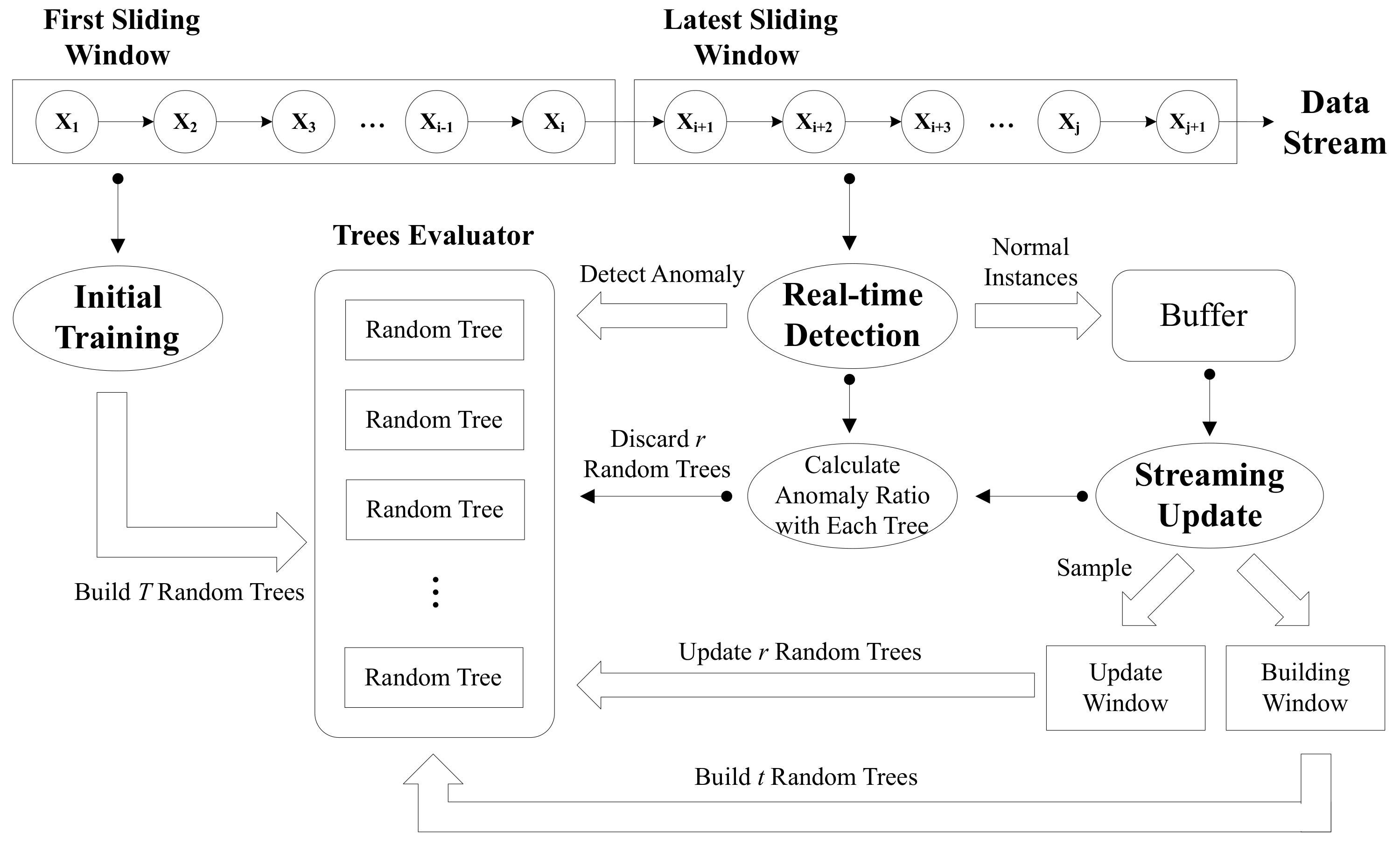
The unsupervised incremental anomaly detection method based on the tree ensemble proposed in this paper consists of three stages: Initial training, real-time detection, and streaming update. The overall workflow is shown in Figure 1. In the first part of the section, we introduce the initial training process. The second part delivers the implementation of detection. Finally, the streaming update is explained in detail in the third part.
3.1. Initial Training
Online processing and mining for real-time data is generally not an evaluation of all historical data, but only the latest data in the stream. Setting a sliding window on the data stream has some attractive features that confine the data to a recent specific range with a special emphasis on the latest information [18], which is more important than the old data in most applications. There are two common types of sliding windows: Time-based and count-based. With the passage of time and the arrival of new instances, both types of sliding windows slide forward, making the data in the window change constantly. Considering the ensemble and the subsample of a fixed size in the analysis of data streams, we chose the count-based sliding window.
In the initial training phase of the model, a sliding window is created to wait for incoming data to flow in. When the sliding window is full, we perform random sampling with replacement of the data in the sliding window for T times and obtain a data block composed of m instances each time, where . Finally, a set with T data blocks is generated. Each block in is first put into the root of a binary tree. Then, the branching process of the tree begins by randomly selecting a dimension among the d-dimensional features of the data and then randomly selects a value v within the maximum and minimum values of the dimension. The instances whose values in dimension are less than v are placed in the left branch of the current node, and those greater than v are placed in the right branch. In this way, the data points of the current node are divided into two subspaces. The same random selection and division processes are performed recursively in these two subspaces, and the division stops when any of the following conditions is reached: (i) The subspace has a single instance, (ii) the binary tree reaches the predetermined depth limit, and (iii) all instances in the subspace have the same values. Note that the depth limit is set to the average height of a tree containing up to m leaf nodes, which is [19]. The branch nodes and the leaf nodes that reach the depth limit need to store the number of instances that fall into them. Considering online tree growth, the leaves that have not reached the maximum depth need to store the specific values of instances in addition to their numbers, as depicted in Algorithm 1. At this point, a random binary tree is constructed based on a data block containing m instances, and other trees are created in the same way. After building T random trees, the training is complete. The ensemble consisting of these trees will be used to evaluate the anomalies of the subsequent data streams.
| Algorithm 1 |
|
3.2. Real-Time Detection
In our method, the entire sliding window is emptied after all random trees have been constructed using the data in the first sliding window. Subsequent data keeps coming, and the sliding window keeps moving forward. At this time, the oldest data in the window will be cleared. In the real-time detection stage, the ensemble evaluator is applied to each new observed point and immediately determines whether it is abnormal. In view of the ’few and different’ characteristic of anomalies, especially in the practical scenarios of ICS, the concept of ’isolation’ was first introduced and applied to anomaly detection in [20]. Because the density of anomalies in the subspace is much lower than that of normal instance clusters, the anomalies can be ’isolated’ with only a small number of splits. This situation is manifested in that the segmentation of anomalies stays close to the root of a binary tree, while the normal instances stay close to the maximum depth.
The common method for detecting anomalies is to sort by the path lengths or anomaly scores of the data points. The path lengths or the depths of an instance x are measured by the number of edges that x traverses for each random binary tree in the ensemble from the root node to the terminated node according to the Depth First Search (DFS) recursive algorithm. Finally, the anomaly score is assigned based on the average depth of the instance in all trees. The average depth will be converted to an anomaly score using Equation (1), given in [20]:
where is the average of the depths of an instance x in all trees, is the normalization factor defined by the average path length of an unsuccessful search in the Binary Search Tree (BST), given the number of data n:
where is the harmonic number, which can be estimated by (Euler’s constant). In general, the anomaly score tends to be 1 when approaches 0, and the data point x is most likely to be abnormal; conversely, the anomaly score tends to be 0 when approaches 1, and x is considered to be normal.
In the production environments of ICS, most of the data are normal, while only a very small part includes anomalies. The sudden surges of anomalies at a moment is a small-probability event, and, thus, it can be considered that the anomaly proportion of the data in the first sliding window during the initial training process is approximately equal to that of the historical operating data in ICS. Similarly, the threshold of the anomaly score of the two can also be obtained by referring to the quantile of the anomaly proportion of the historical set, that is:
where is the quantile function, is the evaluation function of the ensemble evaluator, X is the historical operating data of the system, and is the proportion of anomalies in X. We consider the instances corresponding to the anomaly score benign, and those corresponding to anomalous.
3.3. Streaming Update
The GR-Trees algorithm combines an update trigger, tree online growth, and mass weighting to continuously incorporate new data information into the existing model and to realize incremental learning for data streams. The update trigger decides when to update the ensemble evaluator based on the abnormality of the data in the sliding window. In GR-Trees, the structure of the tree is not static, but new branches will grow according to the characteristics of the data stream, and the new branches will affect the detection result and make it more accurate. The tree online growth and mass weighting mechanisms ensure that the detection model can be adjusted in time as the data distribution changes to avoid misjudgments caused by concept drift. Since only some leaf nodes in each random tree store a small amount of information, this method requires less memory consumption and has better storage performance.
3.3.1. Update Trigger
The ensemble evaluator consisting of random binary trees has been constructed in the initial training phase. For the subsequent data streams, the evaluator determines whether their status is normal or abnormal. Then, a buffer is created to collect all normal instances in the sliding window. When the number of data in the buffer is greater than the threshold , the ensemble evaluator begins to update. The update process first randomly samples data from the buffer and uses them to optimize the ensemble estimator, including the online growth of trees and the replacement of old trees with new trees in the ensemble. Meanwhile, the sliding window and buffer are emptied in preparation for the new data.
3.3.2. Online Growth of Trees
A tree-update window and a tree-building window are required in this process. Given data sampled from the buffer, m instances (same as the subsample size in constructing a random binary tree) are randomly selected from them to enter the update window; these constitute the dataset for online growth of trees. The remaining instances are put into the building window to construct new trees. The number of trees that can grow online is determined as:
where T is the ensemble size, is the proportion of the trees with growth in the ensemble, and is the round-up operation. means that the ensemble remains in the original state and that any tree in it will not grow; , that is, , means that t trees from the ensemble are randomly selected and made to grow using . After this process is done, the update window is cleared.
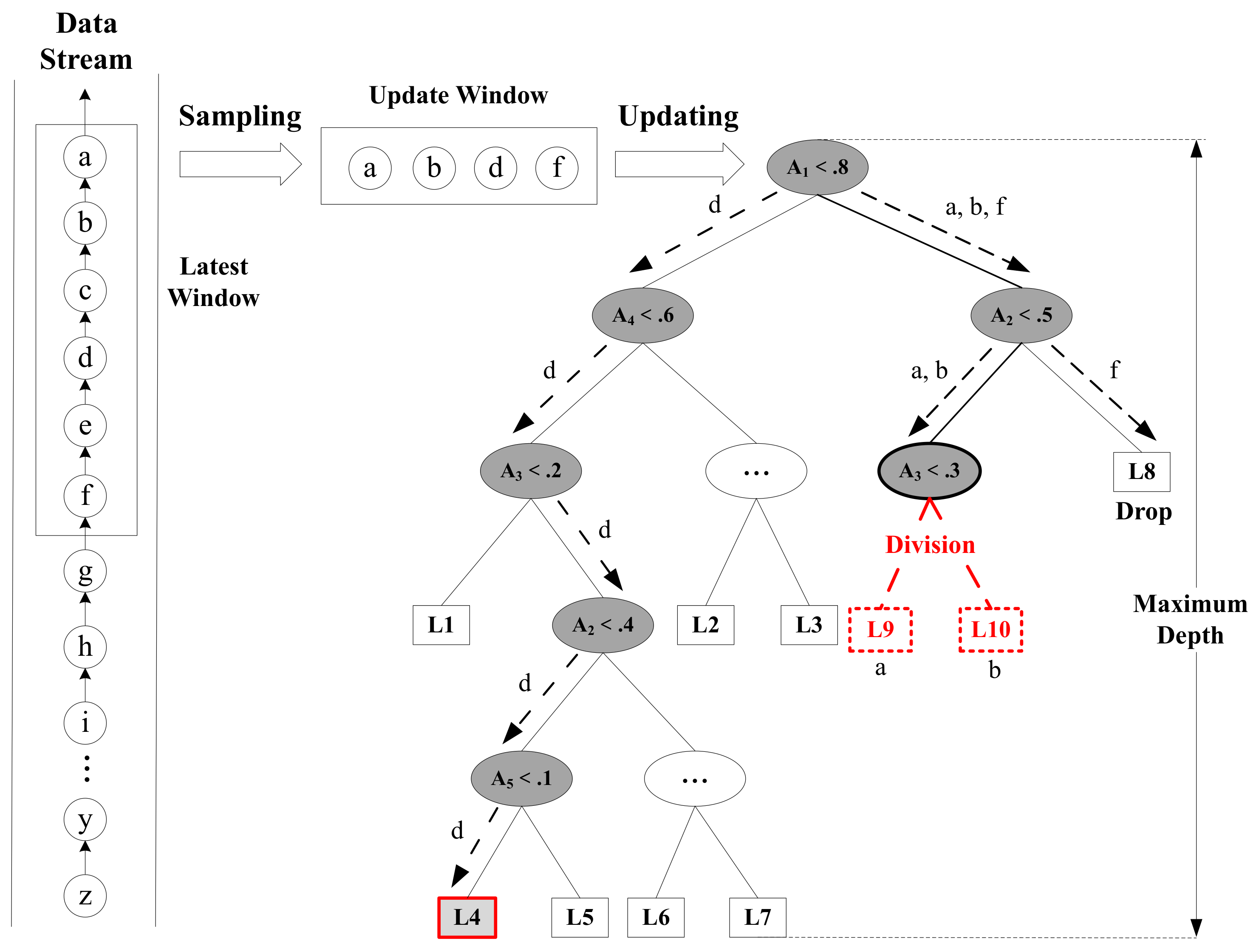
The online growth process of a tree is as follows: For each instance in , traverse down random binary tree following the training rules and find the leaf nodes where they fall in. If the depth of the current leaf node is less than the maximum depth and the values of new instances are different from those of the original data contained in the node, the leaf node divides with a certain probability; otherwise, it does not divide. If the current leaf node reaches the depth limit, the number of data recorded in the node will be updated. Figure 2 depicts an example of a single tree growing online. In [9], anomalies are more likely to be isolated than normal instances. Therefore, nodes with smaller depths in the tree tend to be in the subspace where anomalies are located, while nodes with closer depths to the maximum depth are more likely to be in the subspace where the normal instances are located. In order to increase the difference between the adjusted depths of normal instances and anomalies in the tree so as to better distinguish the two, the node division strategy adopted in this paper is that the division probability increases with the increase of the depth of the leaf nodes, that is, nodes with larger depths have a higher probability of splitting than those with smaller depths. Whether a leaf node can be split depends on the following formula:
where is the division probability of node i, is the depth of node i in the tree, and is the maximum depth.
Node division is the same as the initial training phase. In the new set composed of new data and old data of the node, a dimension is randomly specified, and a value is randomly generated between the maximum value and minimum value of the selected dimension in this set as the dividing point. If the instances in the new set are smaller than the dividing point in the specified dimension, then those instances are sent to the left branch; otherwise, they are sent to the right branch. This division process is performed recursively on the two branches until a single instance is isolated, the depth limit is reached, or all of the values in a node are the same. It can be seen that a tree creates new branches and adjusts the weights of leaves following this node division strategy. Details of the online growth of trees can be found in Algorithm 2.
| Algorithm 2 Online Growth of Trees |
|
3.3.3. Mass Weighting
Although the online growth of random binary trees makes the normal instances and anomalies more distinguishable in adjusted depth in the tree, as new data are continuously added to the tree, the number of points recorded in the leaf nodes of some trees will far exceed that of other trees at the same depth, thereby disrupting the balance of the ensemble to some extent. In this case, the solution is to discard the tree once it has a leaf node that contains more instances than the threshold; this is because the structure of this tree is too far from the ensemble structure, which is no longer applicable for evaluating the path lengths of instances. We set this threshold to be the subsample size because the leaf node contains a maximum of m data points in a tree constructed with m samples. Considering the most extreme case where a binary tree is fully grown online, the number of leaf nodes is m, and each leaf node contains m data instances, so the binary tree needs to record instances. Furthermore, for an ensemble of T trees, the maximum number of data points that need to be stored is . Storing these data points is easy to implement, and such a memory space requirement is trivial in modern equipment.
For some application scenarios, the distribution of data samples might drift to varying degrees over time, and some old information should be allowed to be unlearned or previously learned knowledge to be revised. Therefore, it is necessary to discard trees from the ensemble and create new trees. However, if we discard trees whose detection results deviate from the ensemble average [21], the distribution of results in the original ensemble will be destroyed and their degree of aggregation will be higher and higher. Finally, the detection results of all trees in the ensemble will tend to be the same. We call this situation positive feedback. In order to avoid the positive feedback caused by rejecting trees and to ensure that the detection result of the ensemble remains relatively stable, we quantitatively discard trees from the ensemble based on the mass weight of the results evaluated by each tree for the sliding window.
In order to calculate the anomaly ratio(R) of data in the sliding window with each tree evaluator in the ensemble, R is defined as:
where and are the number of anomalies and the total number of all instances in the current sliding window, respectively. The anomaly ratios of the sliding window obtained by T tree evaluators constitute a set . Then, the maximum value and minimum value are taken from and the interval consisting of and is divided into N segments. We can write the boundary values of each interval as
where is the length of each segment; it is equal to . Then, we can easily count the number of anomaly ratios that fall within each interval, which form the set with , and, finally, the proportion of the tree that should be discarded in the interval i is . Therefore, old trees are randomly selected at each interval, and then these trees are replaced with new ones.
The instances in the buffer enter the tree-building window and form the dataset , which is used to create new trees (see Section 3.3.2). In the same way as in the initial training process, we sequentially perform sampling with replacement, random selection, and partitioning to build a new random binary tree using . Finally, the building window will be emptied.
After all of the above steps have been completed, we have implemented the update of the entire ensemble evaluator. The new tree ensemble (Algorithm 3) is used to detect the subsequent data streams, and the feedback results will in turn update the ensemble evaluator.
| Algorithm 3 Mass Weighting |
|
4. Experimental Evaluation
The purpose of our experiment is to compare the performance of the incremental anomaly detection method in this paper, GR-Trees, and its offline counterpart. We also verify how much of a positive effect the online growing procedure has had on our method. In addition, we examine the impacts of different parameter settings on the detection results of GR-Trees.
4.1. Evaluation Criteria
The confusion matrix is the most basic, intuitive, and easiest way to measure the accuracy of the classification model. The general parameters for model evaluation can be calculated from the confusion matrix: Accuracy, Precision, Recall, F1 score, and Specificity. Accuracy represents the overall prediction accuracy, including positive and negative samples; precision represents the prediction accuracy of positive sample results; specificity is used to measure the ability of the classifier to recognize negative samples; recall is for the original sample, and it indicates the probability of being predicted to be a positive sample in the actual positive samples; the F1 score is the weighted harmonic average of precision and recall, which can make both reach higher values at the same time. Therefore, the F1 score is a comprehensive evaluation index of model accuracy.
However, the number of anomalies is usually much smaller than normal samples in anomaly detection. If the above indicators are used to evaluate the model, the problem of sample imbalance will cause the final results to be inconsistent with the basic facts of the actual situation. Thus, we use AUC (Area Under the receiver operating characteristic Curve) as the scale to measure our method, which is obtained by expanding on the basis of recall and specificity. Because AUC is based on the results of actual performance and observes the related probability problems in the actual positive and negative samples, it avoids the bias of the evaluation results caused by the imbalance of the samples.
4.2. The SWaT Dataset
SWaT (The Secure Water Treatment) is a water treatment testbed for network security research [22]. It is a unique and complex facility that simulates the functions of water treatment systems in the real world. The SWaT dataset contains the network traffic and physical properties derived from 11 days of continuous operation. For the first seven days, the system was under normal operation, while for the next four days, it suffered certain cyber and physical attacks. The physical properties were obtained from different sensors and actuators available in SWaT, and the network traffic was captured from the communication between the SCADA system and the PLCs. The attacks were launched by hijacking the packets used in communication and tampering with their values. During this process, the network packets were modified to reflect the spoofed value from the sensors. We chose network traffic in the SWaT dataset to evaluate the performance of the proposed anomaly detection method. Each network connection is labeled as normal or attack.
The original network traffic in the SWaT dataset contains 11 days of operating data. The daily data consists of 70 CSV(Comma-Separated Values) files, each of which comprises 500,000 pieces of network connection information. However, as the data were captured at a per second interval, there are overlapping instances where multiple pieces of data information with the same timestamps reflect a different activity. We chose the data collected on 31 December 2015. During this day, the system encountered four different types of attacks in four different periods, and the types of attacks in each period were the same. We first removed redundant records and records with missing information in the original data [23], and then extracted 600 thousand normal traffic instances and 60 thousand abnormal traffic instances according to collection time to form the experimental dataset, where anomalies were divided into four different types.
4.3. Results and Analysis
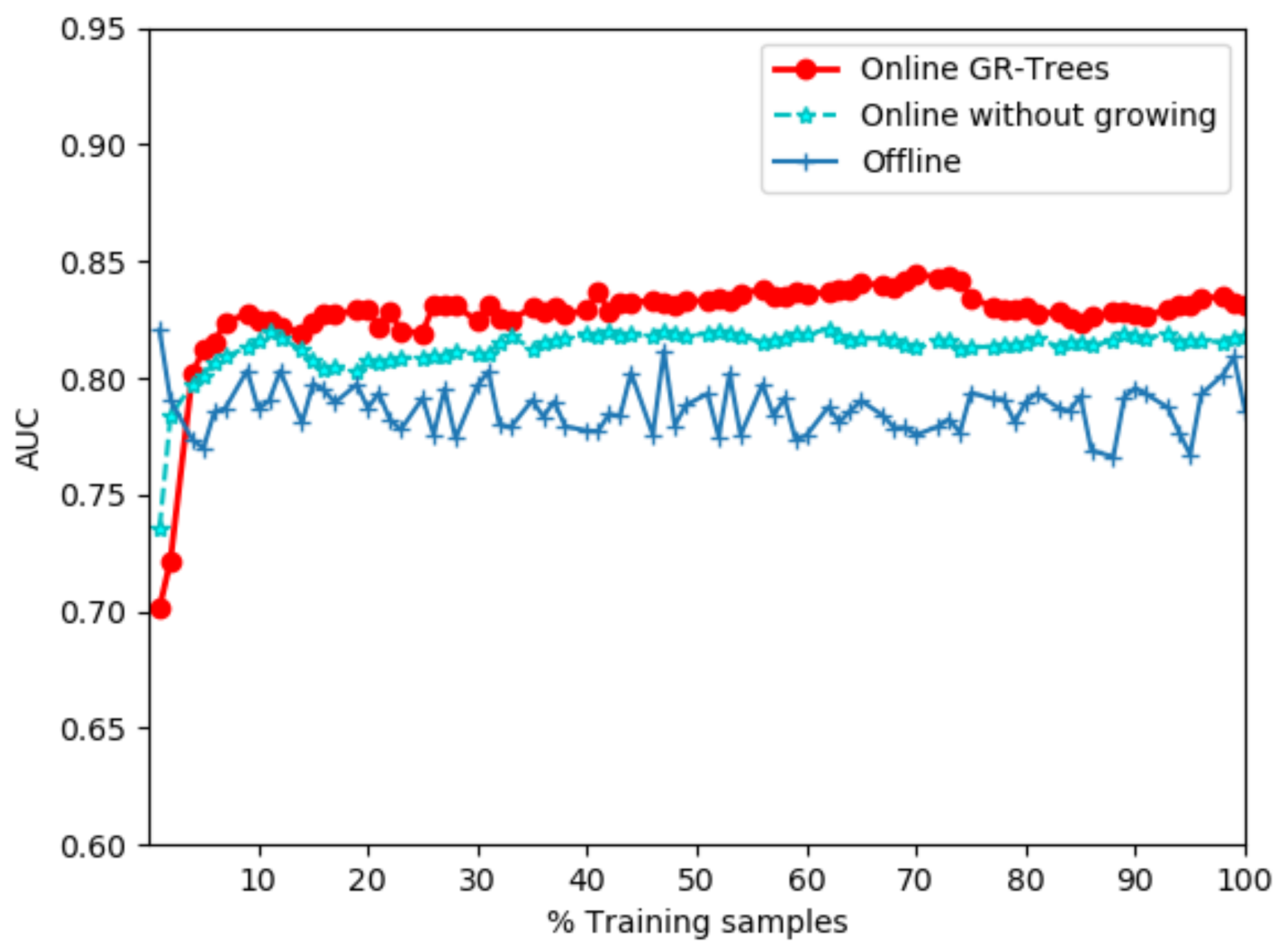
We used the SWaT network traffic dataset to evaluate the detection performance of GR-Trees, its offline counterpart [20], and an online model without growing that only constructs new trees to replace old ones based on mass weight. For this experiment, we set the number of trees to be 100 and the subsample size to be 256. We set and for the streaming update. Figure 3 compares the fluctuation of AUC scores for these three methods as the number of training samples from the SWaT dataset changes. We can see that the overall AUC scores of GR-Trees and the online model without growing are higher than the offline model, which illustrates the importance of gradually updating the model. In the initial stage, GR-Trees does not perform as well as the online model without growing. This difference is caused by the randomness of selection of features and feature values during tree construction. As the number of training samples increases, that is, the data stream is successively obtained, the positive effect of online tree growth gradually becomes apparent, leading to the AUC score of GR-Trees gradually exceeding the latter and continuing to maintain this advantage.
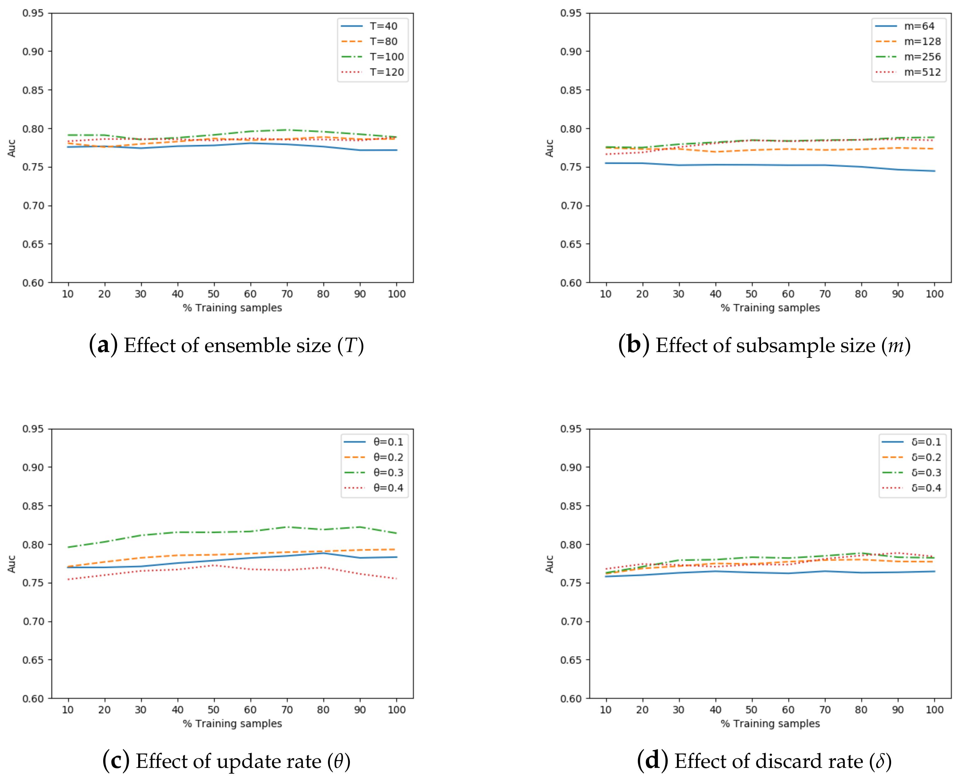
The parameters that have an important influence on the accuracy of our method are the ensemble size, subsample size, update rate, and discard rate. Other parameters, such as buffer threshold, mainly affect how often the ensemble evaluator is updated; nevertheless, they are not the focus of our attention. Figure 4 shows the effects of different ensemble sizes, subsample sizes, update rates, and discard rates.
In Figure 4a, we show the change in the AUC score when the ensemble size (T) is 40, 80, 100, and 120, respectively. The increase in ensemble size within a certain range is conducive to improving the AUC score. However, when it exceeds 100, the AUC score does not change obviously. In terms of experimental results, we shall use as the default value in our experiment.
Figure 4b depicts the impacts of different subsample sizes (m)—64, 128, 256, and 512—on the detection performance. As the size increases in the range of 64 to 128, the overall AUC average increases significantly. Setting the subsample size to 256 or 512 achieves similar results. Therefore, if it is observed that the subsample reaches a certain scale and its size has little effect on the performance in actual applications, then it is not necessary to increase the subsample size because it will only increase the processing time and storage requirements of the system without major performance improvements. A subsample of 256 instances is more appropriate for creating a random binary tree and detecting anomaling in our method.
Considering the speed and performance of the method, we set the values of the update rate () and discard rate () to be less than 0.5, and select some discrete points for experiments. The sets of both are 0.1, 0.2, 0.3, and 0.4 in Figure 4c,d. The AUC of and 0.2 are relatively close, but the latter is slightly higher than the former. When the update rate reaches 0.3, the AUC improves greatly compared with the previous, whereas when increases to 0.4, it decreases to the minimum. Therefore, setting the update rate to 0.3 is nearly optimal in this experiment. As for the discard rate, the worst detection performance is achieved at , while the results at , and 0.4 are better and similar. Empirically, the discard rate can be adjusted between 0.2 and 0.4 according to the actual needs so as to obtain better results.
To further verify the effectiveness of GR-Trees, we evaluated GR-Trees and the corresponding offline algorithm (Isolation Forest, IF) on the Http and Smtp (from KDD Cup 99), ForestCover, and Shuttle (from UCI Machine Learning Repository) datasets. The data distribution features of Http and ForestCover are that a large number of anomalies will burst out during certain periods of the data stream, while the distributions of anomalies in Smtp and Shuttle are relatively uniform. Additionally, since there have not been suitable unsupervised anomaly detection models of the same type with good effects in core journals and conferences in recent years, we chose an online semi-supervised algorithm, Streaming Half-Space-Trees (HS-Trees), for the comparison test. In order to uniformly compare the performances of various algorithms, the overall abnormal proportion of each dataset was constrained to 0.1. According to the above analysis of parameter effects, we used 100 trees, a subsample of 256, , and in GR-Trees. As for IF and HS-Trees, we used their default settings. In all experiments, we independently ran each algorithm 10 times on each dataset and calculated the average AUC as the experimental result. Table 1 summarizes the information of the above four datasets and records the results of the experiments for all methods. From the table, we can observe that the performance of GR-Trees on the three datasets (Http, Smtp, and ForestCover) was better than that of IF; in particular, the AUC scores on the Http and ForestCover were greatly improved, indicating that our method is more adaptable to sudden changes in data than its offline version. Although the AUC of GR-Trees on the Shuttle was slightly lower than that of IF, in general, GR-Trees can achieve comparable results to its offline counterpart. The experimental results also show that GR-Trees has a similar detection performance compared with that of HS-Trees, and GR-Trees even outperforms the latter on the Http, Smtp, and Shuttle datasets.
5. Conclusions
In view of the challenge of rapid analysis of large-scale data streams in the current industrial control system, as well as its realistic demand for unsupervised learning and unbalanced processing of data categories, this paper introduces an unsupervised incremental anomaly detection method based on the ensemble of trees for data streams. We combined an update trigger, tree growth, and mass weighting scheme that allows for online updating and building of random binary trees, achieving the purpose of learning from new data. This method takes full advantage of the low time complexity of the ensemble algorithm of trees and extends it to efficient streaming calculations for mass data while solving the problem that the overall performance of the anomaly detector degrades due to the random updating of the model. Since only a few leaf nodes of each tree store a small amount of data information, it has good storage performance and adaptability to environments with limited memory. The empirical evaluations on the SWaT and several common UCI datasets show that the proposed method can meet the performance of the corresponding algorithm in the offline mode.
Author Contributions
Conceptualization, L.L. and M.H.; methodology, L.L., M.H., and X.L.; software, L.L. and M.H.; validation, L.L.; formal analysis, L.L. and M.H.; investigation, L.L, M.H., and C.K.; resources, C.K. and X.L.; writing—original draft preparation, L.L. and M.H.; writing—review and editing, C.K. and X.L.; supervision, X.L.; project administration, C.K. and X.L.; funding acquisition, C.K. All authors have read and agreed to the published version of the manuscript.
Funding
This research was funded by the project "Research on Key Technologies of Trusted Analysis and Defense of Business Security in Distribution Automation System (PDB 17201800158)" of the State Grid Corporation of China, and was partly supported by the National Nature Science Foundation of China (61672111).
Acknowledgments
The authors would like to convey their heartfelt gratefulness to the reviewers and the editor for the valuable suggestions and important comments which greatly helped them to improve the presentation of this manuscript.
Conflicts of Interest
The authors declare no conflict of interest.
References
- Lee, J.; Bagheri, B.; Kao, H.A. Recent advances and trends of cyber-physical systems and big data analytics in industrial informatics. In Proceedings of the IEEE 12th International Conference on Industrial Informatics (INDIN), Porto Alegre, Brazil, 27–30 July 2014; pp. 1–6. [Google Scholar]
- Babcock, B.; Babu, S.; Datar, M.; Motwani, R.; Widom, J. Models and Issues in Data Stream Systems. In Proceedings of the Twenty-first ACM SIGMOD-SIGACT-SIGART Symposium on Principles of Database Systems, Madison, WI, USA, 3–5 June 2002; pp. 1–16. [Google Scholar] [CrossRef] [Green Version]
- Zhao, J.; Yang, G.; Mu, L.; Fan, T.; Yang, N.; Wang, S. Research on the application of the data stream technology in grid automation. Power Syst. Technol. 2011, 35, 6–11. [Google Scholar]
- Lim, L.; Misra, A.; Mo, T. Adaptive data acquisition strategies for energy-efficient, smartphone-based, continuous processing of sensor streams. Distrib. Parallel Databases 2012, 31, 1–31. [Google Scholar] [CrossRef] [Green Version]
- Jardine, W.; Frey, S.; Green, B.; Rashid, A. SENAMI: Selective non-invasive active monitoring for ICS intrusion detection. In Proceedings of the 2nd ACM Workshop on Cyber-Physical Systems Security and Privacy, Xi’an, China, 30 May 2016; pp. 23–34. [Google Scholar]
- Aggarwal, E.; Karimibiuki, M.; Pattabiraman, K.; Ivanov, A. CORGIDS: A correlation-based generic intrusion detection system. In Proceedings of the 2018 Workshop on Cyber-Physical Systems Security and PrivaCy, Beijing, China, 26 February 2018; pp. 24–35. [Google Scholar]
- Alzghoul, A.; Löfstrand, M. Increasing availability of industrial systems through data stream mining. Comput. Ind. Eng. 2011, 60, 195–205. [Google Scholar] [CrossRef]
- Muallem, A.; Shetty, S.; Pan, J.W.; Zhao, J.; Biswal, B. Hoeffding tree algorithms for anomaly detection in streaming datasets: A survey. J. Inf. Secur. 2017, 8, 339–361. [Google Scholar] [CrossRef] [Green Version]
- Saffari, A.; Leistner, C.; Santner, J.; Godec, M.; Bischof, H. On-line random forests. In Proceedings of the IEEE 12th International Conference on Computer Vision Workshops, ICCV Workshops, Kyoto, Japan, Kyoto, Japan, 27 September–4 October 2009; pp. 1393–1400. [Google Scholar]
- Tan, S.C.; Kai, M.T.; Fei, T.L. Fast Anomaly Detection for Streaming Data. In Proceedings of the 22nd International Joint Conference on Artificial Intelligence, Barcelona, Spain, 16–22 July 2011. [Google Scholar]
- Galar, M.; Fernandez, A.; Barrenechea, E.; Bustince, H.; Herrera, F. A review on ensembles for the class imbalance problem: Bagging-, boosting-, and hybrid-based approaches. IEEE Trans. Syst. 2011, 42, 463–484. [Google Scholar] [CrossRef]
- Barbosa, R.R.R.; Sadre, R.; Pras, A. Towards periodicity based anomaly detection in SCADA networks. In Proceedings of the 2012 IEEE 17th International Conference on Emerging Technologies & Factory Automation (ETFA 2012), Krakow, Poland, 17–21 September 2012; pp. 1–4. [Google Scholar]
- Ponomarev, S.; Atkison, T. Industrial control system network intrusion detection by telemetry analysis. IEEE Trans. Dependable Secur. Comput. 2015, 13, 252–260. [Google Scholar] [CrossRef]
- Kiss, I.; Genge, B.; Haller, P.; Sebestyén, G. Data clustering-based anomaly detection in industrial control systems. In Proceedings of the 2014 IEEE 10th International Conference on Intelligent Computer Communication and Processing (ICCP), Cluj-Napoca, Romania, 4–6 September 2014; pp. 275–281. [Google Scholar]
- WANG, D.; YANG, L. Stream Processing Method and Condition Monitoring Anomaly Detection for Big Data in Smart Grid. Autom. Electr. Power Syst. 2016, 2016, 18. [Google Scholar]
- Lin, L.; Su, J. Anomaly detection method for sensor network data streams based on sliding window sampling and optimized clustering. Saf. Sci. 2019, 118, 70–75. [Google Scholar] [CrossRef]
- Yang, Y.H.; Huang, H.Z.; Shen, Q.N.; Wu, Z.H.; Zhang, Y. Research on intrusion detection based on incremental GHSOM. Chin. J. comput. 2014, 37, 1216–1224. [Google Scholar]
- Golab, L.; Özsu, M.T. Issues in data stream management. ACM Sigmod Rec. 2003, 32, 5–14. [Google Scholar] [CrossRef]
- Knuth, D.E. Sorting and Searching, Art of Computer Programming, 2nd ed.; Addison Wesley Longman Publishing Co.: Redwood, CA, USA, 1988. [Google Scholar]
- Liu, F.T.; Kai, M.T.; Zhou, Z.H. Isolation Forest. In Proceedings of the 2008 Eighth IEEE International Conference on Data Mining, Pisa, Italy, 15–19 December 2008; IEEE: Washington, DC, USA, 2008; pp. 995–1000. [Google Scholar]
- LI, X.; Gao, X.; Yan, B.; Chen, C.; Chen, B.; Li, J.; Xu, J. An Approach of Data Anomaly Detection in Power Dispatching Streaming Data Based on Isolation Forest Algorithm. Power Syst. Technol. 2019, 43, 1447. [Google Scholar] [CrossRef]
- Goh, J.; Adepu, S.; Junejo, K.N.; Mathur, A. A Dataset to Support Research in the Design of Secure Water Treatment Systems. In Proceedings of the 11th International Conference on Critical Information Infrastructures Security, Paris, France, 10–12 October 2016. [Google Scholar]
- Schneider, P.; Böttinger, K. High-Performance Unsupervised Anomaly Detection for Cyber-Physical System Networks. In Proceedings of the 2018 Workshop on Cyber-Physical Systems Security and PrivaCy, Toronto, ON, Canada, 19 October 2018. [Google Scholar]
Figure 1.
The workflow of unsupervised incremental anomaly detection.

Figure 2.
An example of a single tree growing online. Data points are sampled from normal instances in the sliding window. They are input into a random binary tree, and then traverse the branch from the root node to find the corresponding leaf nodes. The rectangle represents the leaf node and the ellipse represents the branch node, in which the split attribute and split value constitute the division condition. (i) a and b should have fallen into the sibling of , but because the leaf node does not reach the maximum depth, this node needs to split (assuming that the split probability of the node satisfies the condition and the node changes from a leaf to a branch) and create two new leaf nodes and (dotted rectangle), which record a and b, respectively; (ii) f falls into and it overlaps with the data recorded in , then drops it; (iii) d falls into , which reaches the maximum depth, and the number of data recorded in will be updated.

Figure 3.
AUC (Area Under the receiver operating characteristic Curve) scores with respect to the ratio of training samples for online Growing Random Trees (GR-Trees; red solid), the online model without growing (cyan dashed), and the offline model (solid) with an increasing number of training samples from the SWaT dataset.

Figure 4.
Effects of different ensemble sizes, subsample sizes, update rates, and discard rates on the detection performance.
Figure 4.
Effects of different ensemble sizes, subsample sizes, update rates, and discard rates on the detection performance.


Table 1.
AUC scores for GR-Trees, Isolation Forest (IF), and Streaming Half-Space-Trees (HS-Trees).
| Dataset | Points | Dimension | Anomaly | AUC | ||
|---|---|---|---|---|---|---|
| GR-Trees | IF | HS-Trees | ||||
| Http | 567,497 | 3 | 0.4% | 0.9502 | 0.5318 | 0.9203 |
| Smtp | 95,156 | 3 | 0.03% | 0.8313 | 0.8255 | 0.8259 |
| ForestCover | 286,048 | 10 | 0.9% | 0.5814 | 0.5293 | 0.6046 |
| Shuttle | 49,097 | 9 | 7% | 0.8923 | 0.9395 | 0.8726 |
© 2020 by the authors. Licensee MDPI, Basel, Switzerland. This article is an open access article distributed under the terms and conditions of the Creative Commons Attribution (CC BY) license (http://creativecommons.org/licenses/by/4.0/).
Share and Cite
MDPI and ACS Style
Liu, L.; Hu, M.; Kang, C.; Li, X. Unsupervised Anomaly Detection for Network Data Streams in Industrial Control Systems. Information 2020, 11, 105. https://0-doi-org.brum.beds.ac.uk/10.3390/info11020105
AMA Style
Liu L, Hu M, Kang C, Li X. Unsupervised Anomaly Detection for Network Data Streams in Industrial Control Systems. Information. 2020; 11(2):105. https://0-doi-org.brum.beds.ac.uk/10.3390/info11020105
Chicago/Turabian StyleLiu, Limengwei, Modi Hu, Chaoqun Kang, and Xiaoyong Li. 2020. "Unsupervised Anomaly Detection for Network Data Streams in Industrial Control Systems" Information 11, no. 2: 105. https://0-doi-org.brum.beds.ac.uk/10.3390/info11020105
Note that from the first issue of 2016, this journal uses article numbers instead of page numbers. See further details here.