Finding the Key Structure of Mechanical Parts with Formal Concept Analysis

1
Department of Computer Science and Technology, Shaoxing University, Shaoxing 312000, Zhejiang, China
2
Department of Mechanical Engineering, Shaoxing Uniersity, Shaoxing 312000, Zhejiang, China
3
College of Mechanical and Electrical Engineering, Shaoxing Uniersity, Shaoxing 312000, Zhejiang, China
*
Author to whom correspondence should be addressed.
Information 2020, 11(2), 116; https://0-doi-org.brum.beds.ac.uk/10.3390/info11020116
Submission received: 20 December 2019
/
Revised: 16 February 2020
/
Accepted: 17 February 2020
/
Published: 20 February 2020
Abstract
:Aiming at the problem that the assembly body model is difficult to classify and retrieve (large information redundancy and poor data consistency), an assembly body retrieval method oriented to key structures was presented. In this paper, a decision formal context is transformed from the 3D structure model. The 3D assembly structure model of parts is defined by the adjacency graph of function surface and qualitative geometric constraint graph. The assembly structure is coded by the linear symbol representation of compounds in chemical database. An importance or cohesion as the weight to a decision-making objective on the context is defined by a rough set method. A weighted concept lattice is introduced on it. An important formal concept means a key structure, since the concept represents the relations between parts’ function surfaces. It can greatly improve the query efficiency.
1. Introduction and Problem Statement
Currently, engineering drawing retrieval is mainly text-based, which makes full use of spatial relationships and properties of components between these geometric elements. Berchtold and Kriegel [1] developed the S3 system, which is a text-based retrieval system and supports local similarity search. The S3 system mainly relies on matching the contour of the graphics, while the spatial relationships are ignored. Therefore, this search method is not suitable for complex graphics. Muller and Rigoll [2] put forward a new stochastic model retrieval method, using a pseudo 2D hidden Markov model (P2DHMM). This method only supports a simple graphic search, but it is not suitable for complex graphics. Park and Um [3] proposed a complex 2D mechanical parts drawing method based on the shape of the key features. It is difficult to handle a large number of engineering drawings because of the minimum geometric components and non-efficient matching algorithm.
The similarity computing is a key issue in the engineering drawings retrieval. It is closely related to feature extraction [4]. Wang and Jiang [5] studied a retrieval method based on graph matching. The method extracted features of the structures and the shapes. Then, the pattern matching problem was transformed into a graph and sub-graph isomorphism problem. Sub-graph isomorphism has been proven to be an NP-complete problem. The time complexity of the algorithm is relatively high, and the performance of the existing solution is unstable.
Zehtaban and Roller [6] developed a shape-based symbol code Opitz and a comprehensive similarity comparison toolbox by two different techniques for data retrieval. Opitz code structure is selected as the grouping technique to classify and regulate geometric information of the CAD model. One of the main challenges in this work is to accurately extract the GT code according to the request. Another challenge is the quality of the code generated by Opitz.
Xu and Dong [7] proposed a parts retrieval method based on similar structures. The parts geometry drawings are marked as functional surfaces. If they have a common edge, a common point or points on the edge, the functions surfaces are topologically connected. A 2D parts structure model is produced by the functional relations. They defined the “and” operation restricting common vertexes and common edges to construct a 3D parts structural model. The codes of parts structure drawings are generated by linear symbols draw representation of the chemical compound database. Through expressing the request using Boolean model of parts drawing sub-structure, matching the sub-structure code and branch structure codes, it is used to retrieve parts drawings. By comparing the overall structure codes of parts drawings with one of the 3D part model, the parts drawings model retrieval is accomplished. In this way, it is required that the user is familiar with the structures of the abstract codes. It is time-consuming and inefficient when dealing with complex and large quantities of engineering drawings.
The concept lattice theory (Formal Concept Analysis FCA) was first proposed by Wille in 1982 as a mathematical theory. Its core is the formal concepts based on the binary relations between objects and attributes in the formal context [8]. The object set, the attribute set, and binary relations between them are the three elements in the formal context. If the attribute set contains the condition attributes and decision attributes, this formal context is a decision formal context [9]. Concept lattice is becoming a powerful tool to study various decision-making problems since the decision formal context was presented by Zhang in 2005 [10]. Subsequently, various extended decision formal contexts are constantly proposed, such as: fuzzy decision formal context, the real value decision formal context, incomplete decision formal context, etc. [11,12,13,14,15]. The main purpose to propose the decision formal context is for decision analysis for relational data. Along this idea, Shao [16] and Qu et al. [15] studied the rules extraction problem of decision formal context using concept lattice. Wu et al. [11] proposed granulation rule mining methods of the decision formal context by means of granulation calculation. Recently, Li et al. [17] discussed theoretical framework construction problems to extract rules from the decision formal context, and a corresponding method is developed by using the discernibility matrix and Boolean function. The knowledge hidden in a decision formal context can compactly be unravelled in the form of implication rules.
It should be pointed out that, in the recent research on the concept lattice, it is usually assumed that all the intents are equally important, and all the nodes would be generated from the formal context. The consequence is that a large number of nodes would be generated, and hence more storage space occupation and longer building time consumption. (With the sharp increasing of the data to deal with, the amount of concept lattice node constructed from original formal context is enormous, accordingly, requiring the larger storage space and time. At the same time, users are not interested in all the intents composed of all the attribute sets. Furthermore, it takes more time to extract useful knowledge from them). Consequently, the user would take more time to extract knowledge in which he is interested from the overall concept lattice. Therefore, it becomes advantageous to introduce some weights into the intent to capture its importance. Since the value of the weight assigned to the intent quantifies its importance, the user does not need to investigate all the nodes but only those nodes he is interested in. As a result, the knowledge extraction can be accelerated, the storage space can be saved, and the time to get results can be shortened. This is the underlying idea that motivates researchers to propose a weighted concept lattice [10]. This construct inherits a structure of general concept lattices while facilitates extraction of interesting knowledge. In many situations, it is apparent that the attributes are quite different from each other when it comes to their relevance and usefulness in knowledge acquisition. For example, we note that people are more interested in recent transaction data than the past ones. In [18], Zhang et al. introduced a virtual node into the frequent weighted concept lattice (FWCL) to ensure that FWCL is retained to be complete, which is to preserve the existence of each nodes’ infima and suprema in the FWCL. Some theories were provided for further applications of the weighted concept lattice [19,20].
There is a lot of research on concept lattice in graph data mining [21,22], especially using stable emerging molecular patterns and mining convex polygon patterns [23,24]. Exponential explosion makes it difficult to consider the whole concept lattice arising from data; one needs to select the most useful and interesting concepts. In [25], interestingness measures of concepts are considered and compared with respect to various aspects, such as efficiency of computation and applicability to noisy data and performing ranking correlation. A cohesion function is based on the pairwise similarity of objects from an extent.
In Ref. [7], the geometric graph of part engineering drawing is labeled as functional surface. The functional surface which is attached topologically is determined according to the fact that, whether they are in the common edge, or whether they have concurrent or point in the edge, and further the position relationship between functional surfaces is decided. The model retrieval is realized via 3D structure code matching of part engineering drawing and part 3D model.
The present work aims to give a comprehensive study on the application of weighted concept lattice in finding the key structure of mechanical parts. In Section 2, the 3D structural model of the parts and its coding were derived. This derivation naturally leads to a new set of the functional surfaces. In Section 3, a direct mapping method from parts drawing structure model to FCA was considered. Identifying important formal concepts was made in this section. In Section 4, an algorithm to find the key structure was proposed, and some examples were applied to demonstrate the new method. In Section 5, some conclusions were given.
2. Structure Model of Parts
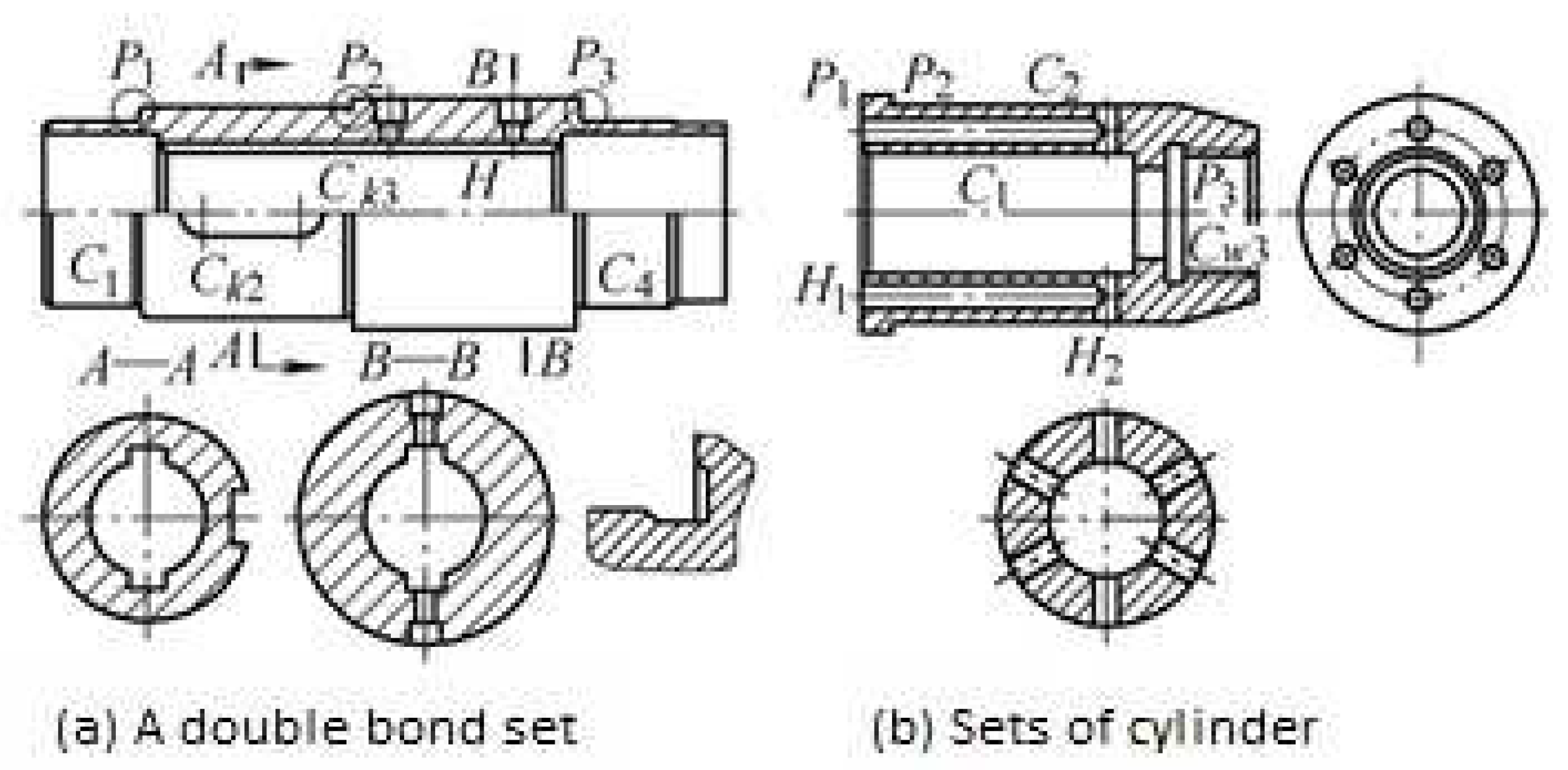
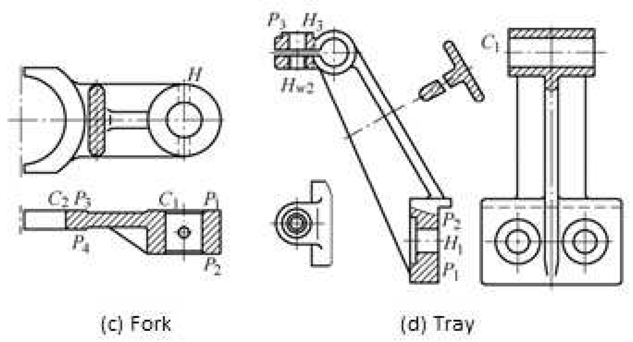
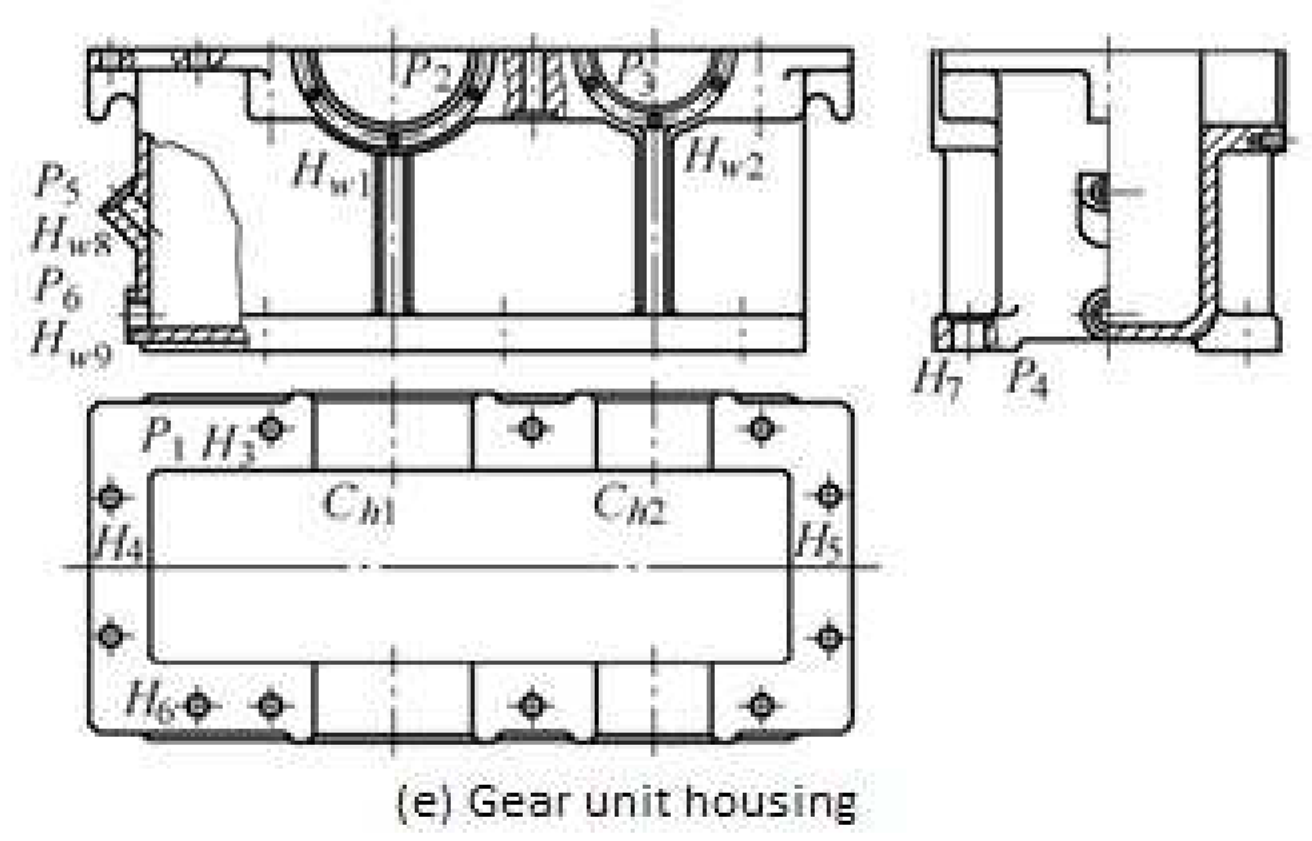
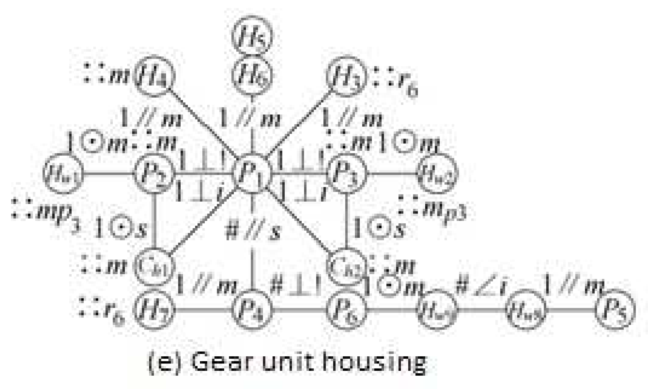
The structural models of part drawings shown in [7] are based on functional surfaces. Basic types of functional surface are planar, cylindrical, conical surface, spherical, and holes. Capital letters , and S represent the planar, cylindrical surfaces, holes and slots, respectively. Lowercase , and r denote the threaded connection, flat key connection, semi-rotary surface, and ring structures.
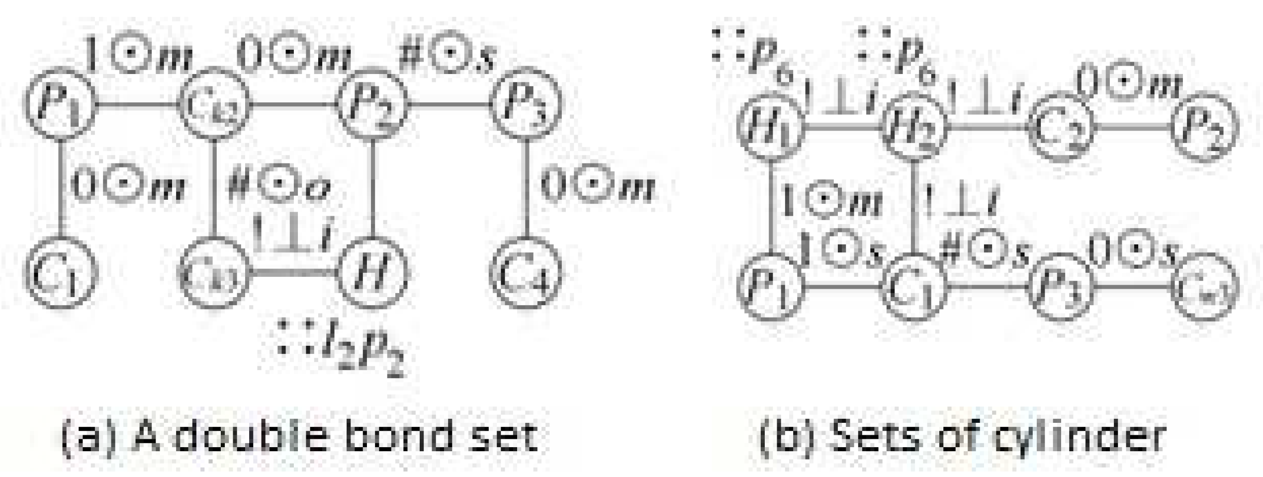
The positional relation between the function surfaces can be represented by vector position relations, including orientation and field relations (see [7]).Topological relations between functional surfaces are represented by concave-convex connection edges: concave side with “0” mark, and the convex with “1”. If the two connected surfaces are revolution ones, the topology can be divided into inner and outer surfaces and use the “!” mark. It can be judged whether the functional surfaces of the part drawings are topologically connected according to three criteria: they have a common edge, a common point, or points in the side. Its basic uses include orientation and domain. The orientation is defined by vectors of geometric space: parallel (||), coaxial (⊙), vertical (⊥), and skew (∠). The domain refers to the relations between the areas that functional surfaces occupy. Table 1 shows the domain relations [7]. The length of the area occupied by the surface of the plane function is 0; therefore, face encounter, overlap, and concurrent are merged into encounters between plane and revolution surfaces. The binary relations between two vertical planes are not defined and marked with the “!” mark. Sign “!♯” represents two functional surfaces being topologically connected, and the symbol “♯” indicates that the topology is not connected. The symbol “?” indicates that the positional relations between the surface features cannot be determined by a single view. The field relations are shown as Table 1.
3. Theory and Method
3.1. Structure Model of Part Drawings Mapping to Concept Lattice
As described above, the main component of the part drawings 3D structural model is the functional surface and their positions. If they are considered as the objects and the attributes, we can build the formal context of the part drawings structure, and then build the concept lattice.
Because the position is for the functional surface of the part, we use “Source” to represent the functional surface of the part, and “Target” to represent the position. Let Source, Relation, and Target be three components of (Parts Graph) with g.source, g.relation and g.target, respectively, the I constitutes (Object, Attribute) sets of the formal context. A formal context consists of a set of objects (g.source), a set of attributes (g.relation and g.target), and a binary relation I that indicates the attributes possessed by each object. There is (g.target, g.source∼ g.relation) . Mapping it makes ’s relations target become a transfer of another relation’s source concept (Concept Graph). This transfer generates implicit map reasoning.
The algorithm works in the following sequence: First, MovingTarget and FixedTarget for each triples are initialized. Second, it calls FormBinaries through all triples iteration. Third, a corresponding formal concept pair (Object, Attribute) is formed. Each time, MovingTarget matches one target concept of the triples. Binary conversion is formed by a recursive call FormBinaries, setting MovingTarget for the current source concept, leaving FixedTarget unchanged.
Using the Algorithm 1, we can get the formal context of part model as shown in Table 2.
| Algorithm 1: A mapping algorithm. |
| begin |
| foreach do |
| FormBinaries(g.target, g.source); |
| end |
| FormBinaries(FixedTarget, MovingTarget) |
| begin |
| foreach do |
| if g.target = MovingTarget then |
| Attribute⟵g.source∼g.relation; |
| Object⟵FixedTarget; |
| (Object, Attribute)}; |
| FormBinaries(FixedTarget, g.source); |
| end |
According to the functional group, for example, group by functional surface of cylinder, hole, plane, and slot, , we can get a decision formal context as described below.
3.2. Weighted Concept Lattice Based on Decision Formal Context
Due to space limitations, we assume that readers are familiar with the basic concepts of formal concept analysis [8].
A formal context can be depicted visually in a tabular form with crosses (or 1) representing the pairs . For example, consider the cross table in Table 3.
The cross table in Table 3 depicts a formal context in which object 1 has attributes a and c, object 2 has attribute a, etc.
Let be a formal context. A set pair of , is a formal concept if and only and , where are common attributes set of all the objects in X and common objects set of all attributes in B, respectively. The set of all formal concepts in is expressed as . Partial order ⪯ of super-concept and sub-concept in constitutes the concept lattice of .
The formal context is the basis of formal concept analysis. Its main objective is to form concepts and concept lattice: The concept is unity of the extension and intension. In essence, the concept lattice describes the link between objects and attributes, indicating generalization relations between concepts, The corresponding Hasse diagram is achieved for data visualization. The traditional concept lattice is based on a simple binary context. In practical application, the data are large and complex. Thus, we must extend it. Belohlávek et al. studied the concept lattice in fuzzy and uncertain data [26,27]. The critical part of concept lattice (called core concepts or important concepts) is an important part of the parts structure. As a user is usually interested in some certain attribute characteristics, according to his/her preference and requirement, the researchers establish a new concept lattice structure with the weight to identify importance of intentions: weighted concept lattice [10].
Example 1.
(,0.6) and (,0.6) are the weighted formal concept formed by the above formal context and single attribute intent weight table. All such formal concepts constitute the weighted concept lattice.
Let be a formal context and a set of attributes is denoted by . are the weights of attributes, where denotes the importance of the attribute . is known as a weighted formal concept on ) if is a formal concept and is the weight of the attribute set . A and B are the extent, the intent of weighted formal concepts, respectively. Its super-concept and sub-concept are the same as the general concept lattice.
Given a value , we can obtain a part of the formal concept , can be seen as a set of important formal concepts.
Definition 1.
[28] Let be a formal context, . is called an attribute set x in B for is called an object set of attribute a for .
Definition 2.
[9] A decision formal context is defined as a quintuple , where and are two formal contexts in which their attribute sets are disjoint. A and D are called condition and decision attribute sets, respectively.
Definition 3.
In a decision formal context , if and and are called the indiscernibility relation determined by the condition and decision attribute, respectively), then is denoted as the equivalence class of object x on B. is the equivalence class of object x on D.
Definition 4.
Let X be a subset of U, .
(1)The lower approximation of X with respect to B is the set of all objects, which can be for certain classified as X with respect to B and it is denoted by . That is, .
(2)The upper approximation of X with respect to B is the set of all objects, which can be possibly classified as X with respect to B and it is denoted by . That is, .
Definition 5.
Let be a decision formal context. If , then we say is consistent.
Definition 6.
In , the lower approximation on the condition attribute B of the decision attribute is . The positive domain of B at the decision-making objective is defined as indicates that there are r decision-making objectives.
Theorem 1.
Let be consistent, .
Proof.
If , then, for any , we have . Since is consistent, it follows that . Then, there exists such that .
If , then, for and , it is clear that . We have . Consequently, . □
Theorem 2.
If be consistent, then a is a core(No-remove attributes).
Proof.
It follows immediately from Theorem 1. □
Definition 7.
For a decision formal context , let be a formal concept of F. The importance of the decision-making objective δ with ) is defined as follows:
It is obvious that .
Example 2.
Computing the importance of concepts: .
In the decision formal context, cohesion of the equivalence classes determined by the condition attributes and decision attributes indicates that the condition attributes impact decision-making, namely the importance of attributes. Next, we will compare attributes of the concept to study the cohesion of the concept to objects (functional surfaces).
The similarity of attributes and can naturally be assessed by the similarity of their corresponding extents, i.e., similarity of and . That is, the similarity measure between attributes and is given by
In our experiments, we use the following functions for on the decision formal context :
, where is the lower approximation of in the decision attribute D. In particular,
(1) If and , then ;
(2) If , then . It produces a computing formula for the general formal context.
Note that is the number of objects that belong to both and classes divided by the number of all attributes that belong to or .
Definition 8.
Cohesion for a formal concept on the decision formal context is defined as the following:
Theorem 3.
The satisfies:
(1) ;
(2) For a formal concept , if and , then .
(3) For a formal concept , if , and , then .
Proof.
(1) Obviously, ; therefore, the conclusion holds.
(2) In fact, for , there exist only two cases , hence, .
(3) Since , it follows from Definition 8 that . Thus, . □
Example 3.
Table 7 is a decision formal context, where is the object set, is the condition attribute set. is the decision attribute set.
, , , . , , , , , , .
A simple approach to measure the cohesion for a formal concept is the following if :
Definition 9.
Let be a decision formal context. is a triple on . If is a formal concept, or is the weight of attribute set B and . is called the weighted concept of . The set consisting of all of these concepts is the weighted concept lattice of .
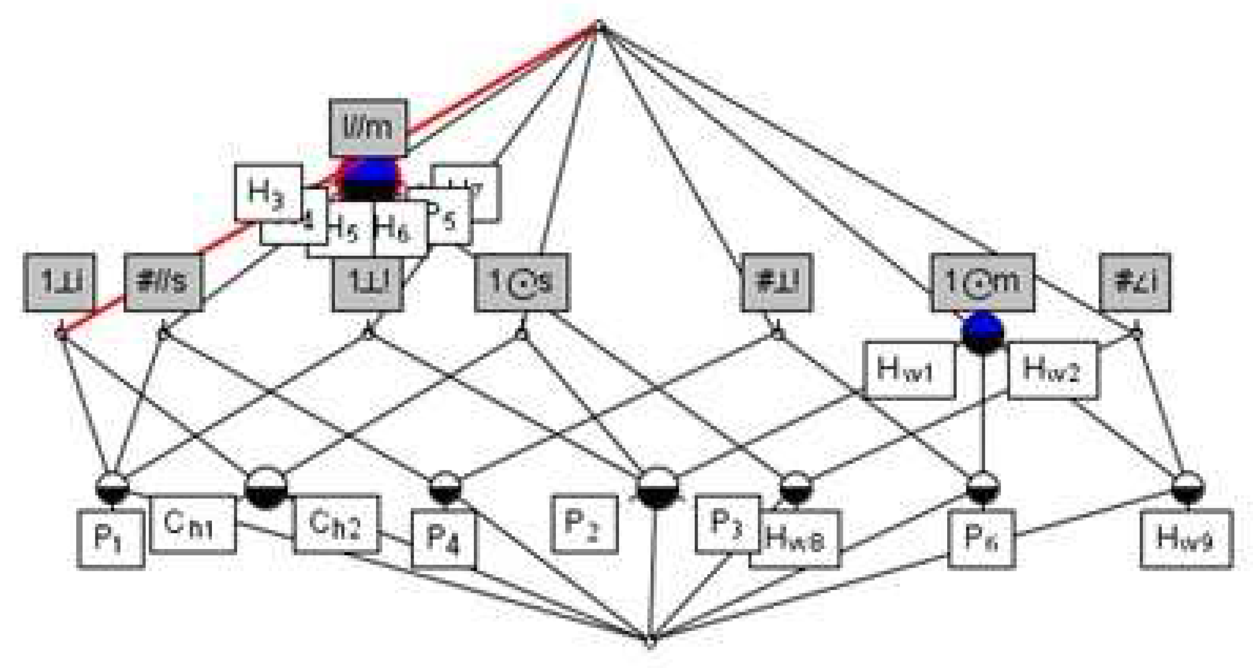
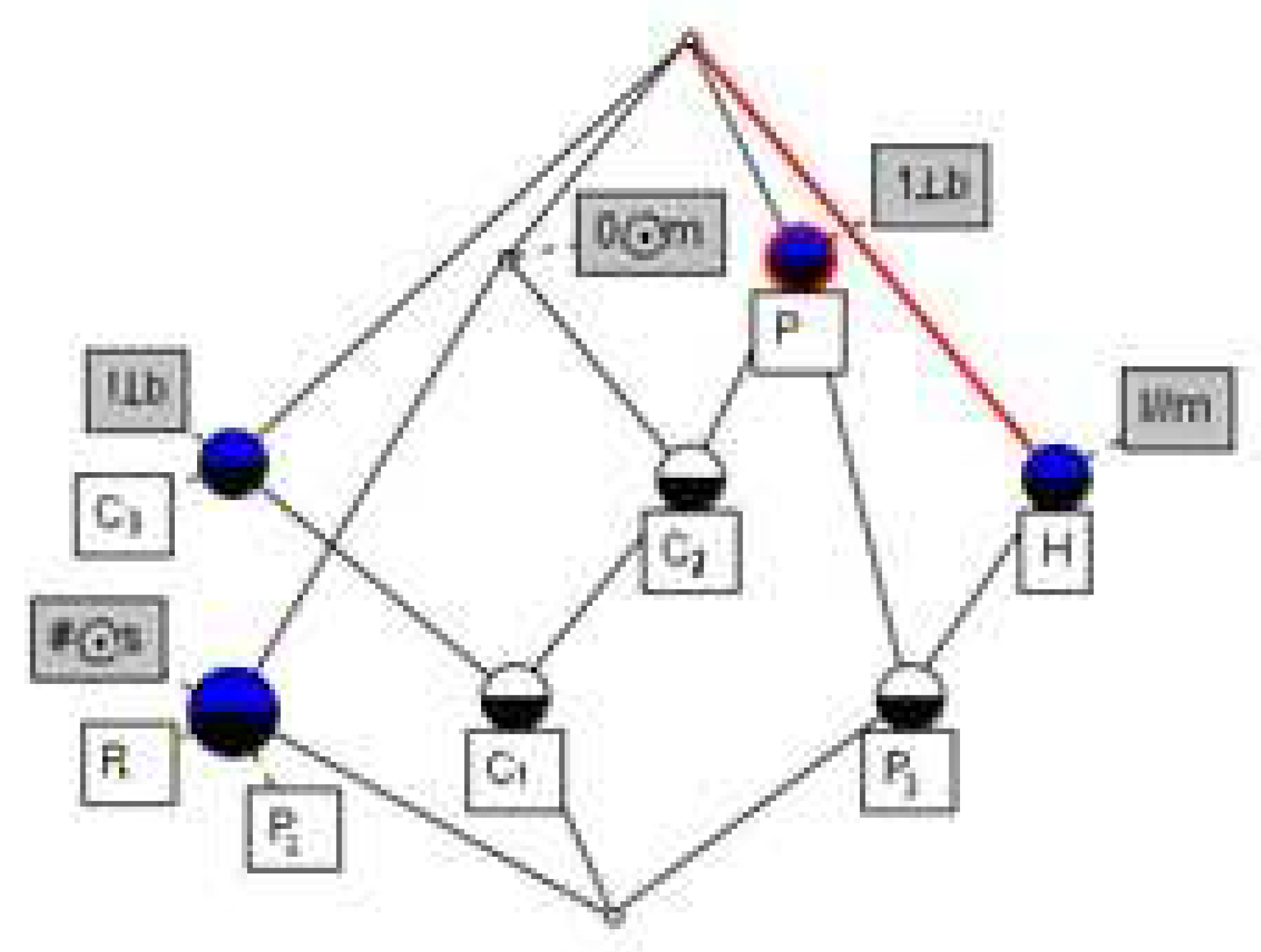
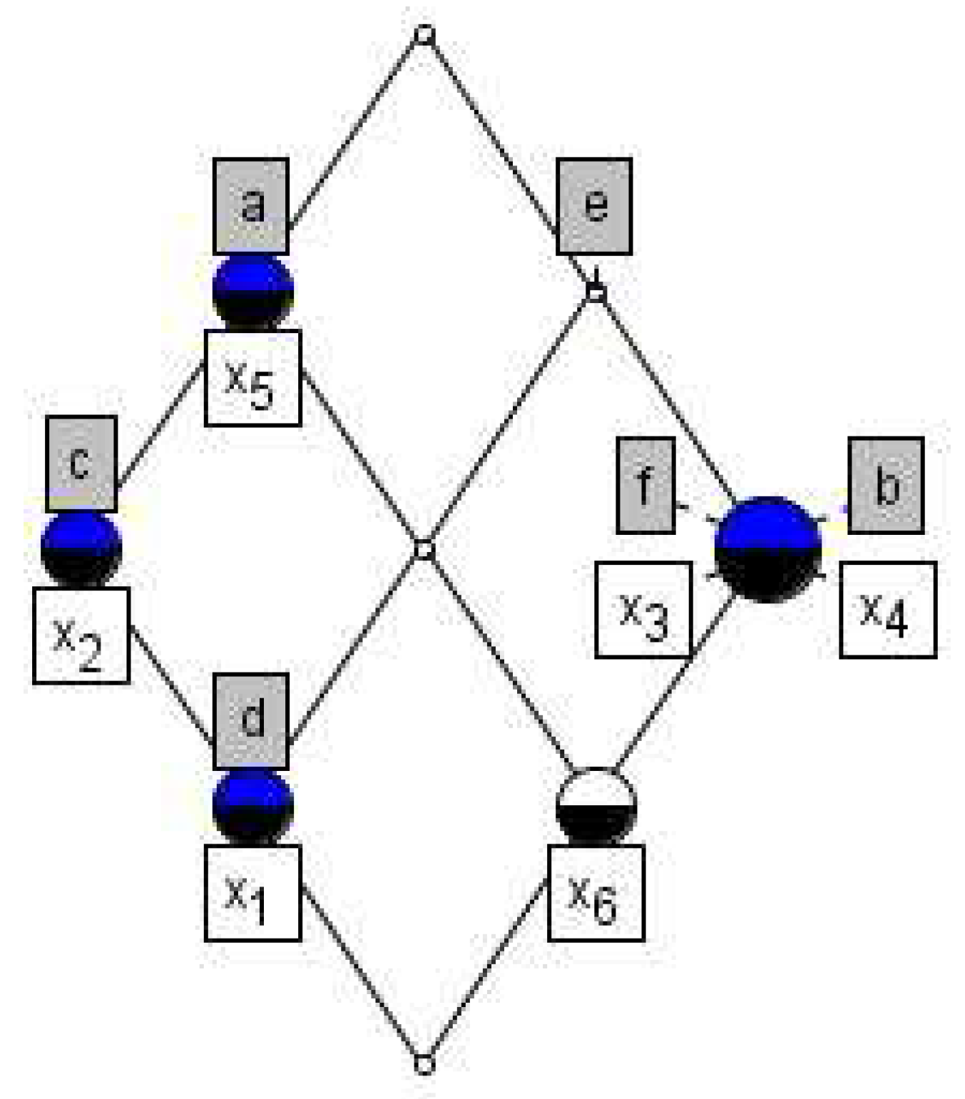
Its formal concept lattice is as Figure 9. Here, the black is an important concept.
4. An Algorithm Getting the Part Key Structure and Examples.
For a formal context transformed from the part drawings structure model, the formal concept is a set pair of the positional relations (the attributes) and function surfaces (the objects). The decision attribute can be seen as the division in which experts think the function surfaces have the same properties (In other words, these functional surfaces play the same role in the part assembly structure). Thus, if given the importance or cohesion value of the concept, to determine important concepts, we can get the part key structure.
In order to verify the validity of the proposed method, five part drawings structure models [7] were calculated individually. Transformed concept lattice and the concept’s extension, intent, and weights are listed below, where concept lattice nodes are denoted by . The weight value marked in red in the table is the key structure (critical concept). If the weight values are all less than , the key structure is the concept node in which w is the closest to (As shown in Table 8, Table 9, Table 10, Table 11 and Table 12 and Figure 10, Figure 11, Figure 12, Figure 13 and Figure 14).
5. Experiments
In order to verify the effectiveness of the method proposed in this paper, the author calculated and compared 7 of the 11 part engineering drawing structural models in Ref. [7]. Here, we set the node of any concept lattice as . If , w is taken as the maximum value, and the important concepts, and key structures of the three-dimensional part structure model as shown in Table 13 can be obtained.
The code of “key structure” in the table is the part drawing structure code from Ref. [7], and the part with red is the key structure calculated by the Algorithm 2 in this paper. From Table 13, it can be seen that, for most parts, the method in this paper can not only determine the important position relation (important intent), but also determine the functional surface (concept object) that constitutes this relationship, and then determine the key structure of parts. Of course, for completely symmetrical parts without “characteristics”, this method also shows limitations (such as pull rod shaft). The reason is that, in these problems, the weight of position relation (concept intent) is exactly the same; that is to say, the information provided by the part drawing itself is not enough to distinguish it. Therefore, as long as the designer provides further information, this problem will be solved.
| Algorithm 2: cAn algorithm of the part key structure with concept lattice searching. |
| Input and |
| begin |
| foreach do |
| Computing w by (1)or (4),compare w and |
| if then next ; |
| else |
| is a key structure; |
| end |
6. Conclusions
This paper has developed a novel scheme for 3D mechanical structure model retrieval. A 3D model is converted into a formal context with the object as the functional surface, and the attribute indicating the positional relations between the functional surfaces. Each concept node contains a topological graph corresponding to the structure that it represents. Integrating the topology and feature structure signatures in FCA not only solves the feature interaction problem, but also accelerates the search process. Due to the significant reduction of the structure number, the graph comparison required in the similarity assessment can be finished in a polynomial time.
This work can be further improved. For example, the structure should consider engineering attributes such as tolerance, fit, and other design descriptions, so that it can capture the user’s intent more accurately. In addition, AI techniques (e.g., fuzzy set, nonlinear neural network) can be applied to determine the weighting factors in our approach more systematically. It ensures that the search scheme properly reflects the user’s intent. Our current research is focused on this.
7. Patents
Qiang Wu: The method and system of key structure modeling of equipment parts based on Weighted Concept Lattice. ZL201610884995.1.
Author Contributions
Data curation, Y.D.; funding acquisition, Y.D.; methodology, Q.W.; writing—original draft, Q.W.; writing—review and editing, L.X. All authors have read and agreed to the published version of the manuscript.
Funding
This work is supported by the National Natural Science Foundation of China (No.51675346).
Acknowledgments
We would like to thank all of the people who have given us helpful suggestions and advice. The authors are obliged to the anonymous referees for carefully looking over the details and for useful comments that improved this paper.
Conflicts of Interest
The authors declare no conflict of interest.
References
- Berchtold, S.; Kriegel, H.P. S3: Similarity search in CAD database systems. In SIGMOD ’97; Association for Computing Machinery: New York, NY, USA, 1997; pp. 564–567. [Google Scholar]
- Müller, S.; Rigoll, G. Searching an Engineering Drawing Database for User-Specified Shapes. In Proceedings of the Fifth International Conference on Document Analysis and Recognition, Bangalore, India, 20–22 September 1999; pp. 697–700. [Google Scholar]
- Park, J.H.; Um, B.S. A new approach to similarity retrieval of 2-d graphic objects based on dominant shapes. Pattern Recognit. Lett. 1999, 20, 591–616. [Google Scholar] [CrossRef]
- Liang, Z.; Qiang, X.; Ding, Q. Engineering drawing retrieval based on graph matching. J. Nanjing Univ. Aeronaut. Astronaut. 2008, 40, 354–359. [Google Scholar]
- Wang, P.; Jiang, S. An engineering drawing retrieval method based on nested assignment algorithm. Mech. Sci. Technol. Aerosp. Eng. 2011, 30, 693–698. [Google Scholar]
- Zehtaban, L.; Roller, D. Beyond similarity comparison: Intelligent data retrieval for cad/cam designs. Comput.-Aided Des. Appl. 2013, 10, 789–802. [Google Scholar] [CrossRef]
- Xu, J.; Dong, Y. Structure retrieval method for part engineering drawing. J. Mech. Eng. 2011, 47, 191–198. [Google Scholar] [CrossRef]
- Ganter, B.; Wille, R. Formal Concept Analysis: Mathematical Foundations; Springer: New York, NY, USA, 1999. [Google Scholar]
- Ganter, B.; Kuznetsov, S.O. Hypotheses and Version Spaces. Lect. Notes Comput. Sci. 2003, 2746, 83–95. [Google Scholar]
- Zhang, J.F.; Zhang, S.L.; Zheng, L. Weighted concept lattice and incremental construction. Pattern Recognit. Artif. Intell. 2005, 10, 171–176. [Google Scholar]
- Wu, W.Z.; Leung, Y.; Mi, J.S. Granular computing and knowledge reduction in formal contexts. IEEE Trans. Knowl. Data Eng. 2009, 21, 1461–1474. [Google Scholar]
- Li, J.; Mei, C.; Lv, Y. Incomplete decision contexts: Approximate concept construction, rule, acquisition and knowledge reduction. Int. J. Approx. Reason. 2013, 54, 149–165. [Google Scholar] [CrossRef]
- Liaab, J. Knowledge reduction in real decision formal contexts. Inf. Sci. 2012, 189, 191–207. [Google Scholar]
- Yang, H.Z.; Yee, L.; Shao, M.W. Rule acquisition and attribute reduction in real decision formal contexts. Soft Comput. 2011, 15, 1115–1128. [Google Scholar] [CrossRef]
- Qu, K.S.; Zhai, Y.H.; Zhao, Y.M. Study of decision implications based on formal concept analysis. Int. J. Gen. Syst. 2006, 36, 533–542. [Google Scholar] [CrossRef]
- Shao, M.W. Knowledge Acquisition in Decision Formal Contexts. In Proceedings of the International Conference on Machine Learning and Cybernetics, Hong Kong, China, 19–22 August 2007; Volume 7, pp. 4050–4054. [Google Scholar]
- Li, J.; Mei, C.; Lv, Y. Knowledge reduction in decision formal contexts. Knowl.-Based Syst. 2011, 24, 709–715. [Google Scholar] [CrossRef]
- Zhang, S.; Guo, P.; Zhang, J.; Wang, X.; Pedrycz, W. A completeness analysis of frequent weighted concept lattices and their algebraic properties. Data Knowl. Eng. 2012, 81–82, 104–117. [Google Scholar] [CrossRef]
- Li, J.; He, Z.; Zhu, Q. An Entropy-Based Weighted Concept Lattice for Merging Multi-Source Geo-Ontologies. Entropy 2013, 15, 2303–2318. [Google Scholar] [CrossRef]
- Zhang, S.; Guo, P.; Zhang, J. Intension weight value acquisition of weighted concept lattice based on information entropy and deviance. Trans. Beijing Inst. Technol. 2011, 31, 59–63. [Google Scholar]
- Kuznetsov, S.O. Learning of Simple Conceptual Graphs from Positive and Negative Examples. Lect. Notes Comput. Sci. 1999, 1704, 384–391. [Google Scholar]
- Ganter, B.; Grigoriev, P.A.; Kuznetsov, S.O.; Samokhin, M.V. Concept-Based Data Mining with Scaled Labeled Graphs. In Proceedings of the International Conference on Conceptual Structures, Huntsville, AL, USA, 18–22 July 2004; Springer: Berlin/Heidelberg, Germany, 2004; pp. 94–108. [Google Scholar]
- Métivier, J.P.; Lepailleur, A.; Buzmakov, A.; Poezevara, G.; Crémilleux, B.; Kuznetsov, S.O.; Le Goff, J.; Napoli, A.; Bureau, R.; Cuissart, B. Discovering Structural Alerts for Mutagenicity Using Stable Emerging Molecular Patterns. J. Chem. Inf. Model. 2015, 55, 925–940. [Google Scholar] [CrossRef]
- Belfodil, A.; Kuznetsov, S.O.; Robardet, C.; Kaytoue, M. Mining Convex Polygon Patterns with Formal Concept Analysis. In Proceedings of the Twenty-Sixth International Joint Conference on Artificial Intelligence, Melbourne, Australia, 19–25 August 2017; pp. 1425–1432. [Google Scholar]
- Kuznetsov, S.O.; Makhalova, T. On interestingness measures of formal concepts. Inf. Sci. 2018, 442–443, 202–219. [Google Scholar] [CrossRef] [Green Version]
- Belohlavek, R. Concept lattices and order in fuzzy logic. Ann. Pure Appl. Log. 2004, 128, 277–298. [Google Scholar] [CrossRef]
- Lubomir, A.; Stanislav, K.; Ondrej, K. On stability of fuzzy formal concepts over randomized one-sided formal context. Fuzzy Sets Syst. 2018, 333, 36–53. [Google Scholar]
- Chen, D.; Zhang, W.; Yeung, D.; Tsang, E.C.C. Rough approximations on a complete completely distributive lattice with applications to generalized rough sets. Inf. Sci. 2006, 176, 1829–1848. [Google Scholar]
Figure 1.
Expression views of several mechanical parts’ functional surfaces (1).

Figure 2.
Expression views of several mechanical parts’ functional surfaces (2).

Figure 3.
Expression views of several mechanical parts’ functional surfaces (3).

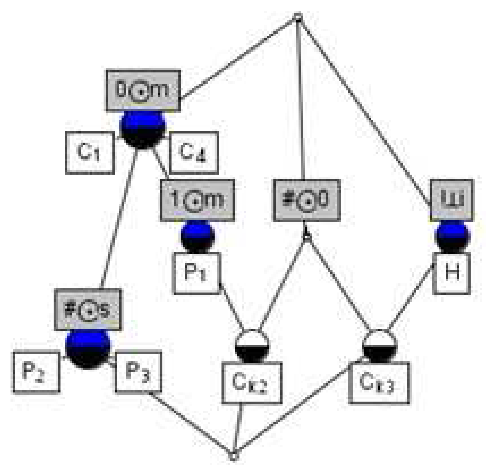
Figure 4.
Figure 1’s 3D structure model.
Figure 4.
Figure 1’s 3D structure model.

Figure 5.
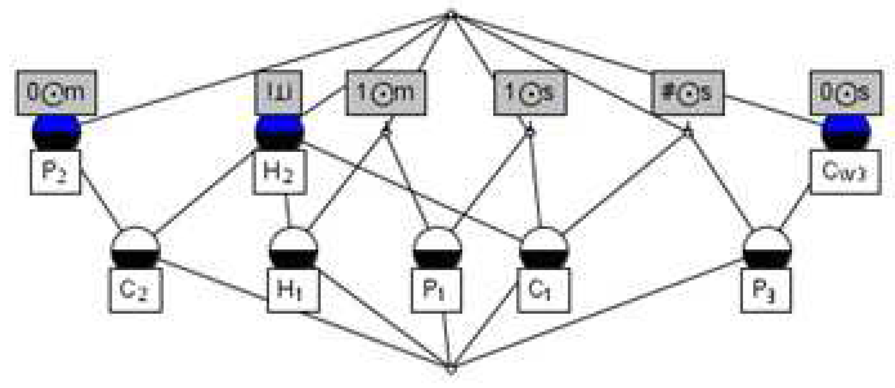
Figure 2’s 3D structure model.
Figure 5.
Figure 2’s 3D structure model.

Figure 6.
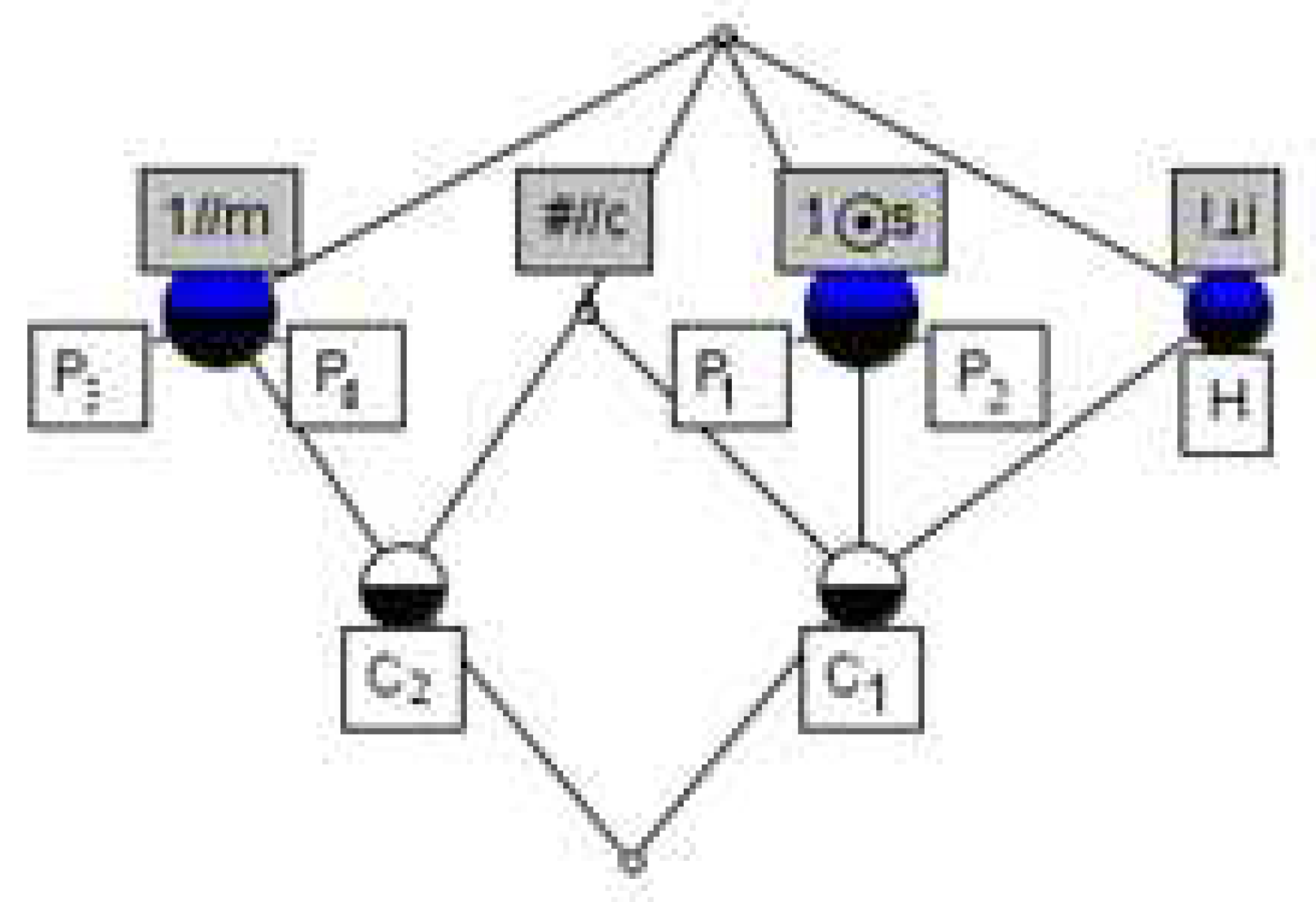
Figure 3’s 3D structure model.
Figure 6.
Figure 3’s 3D structure model.

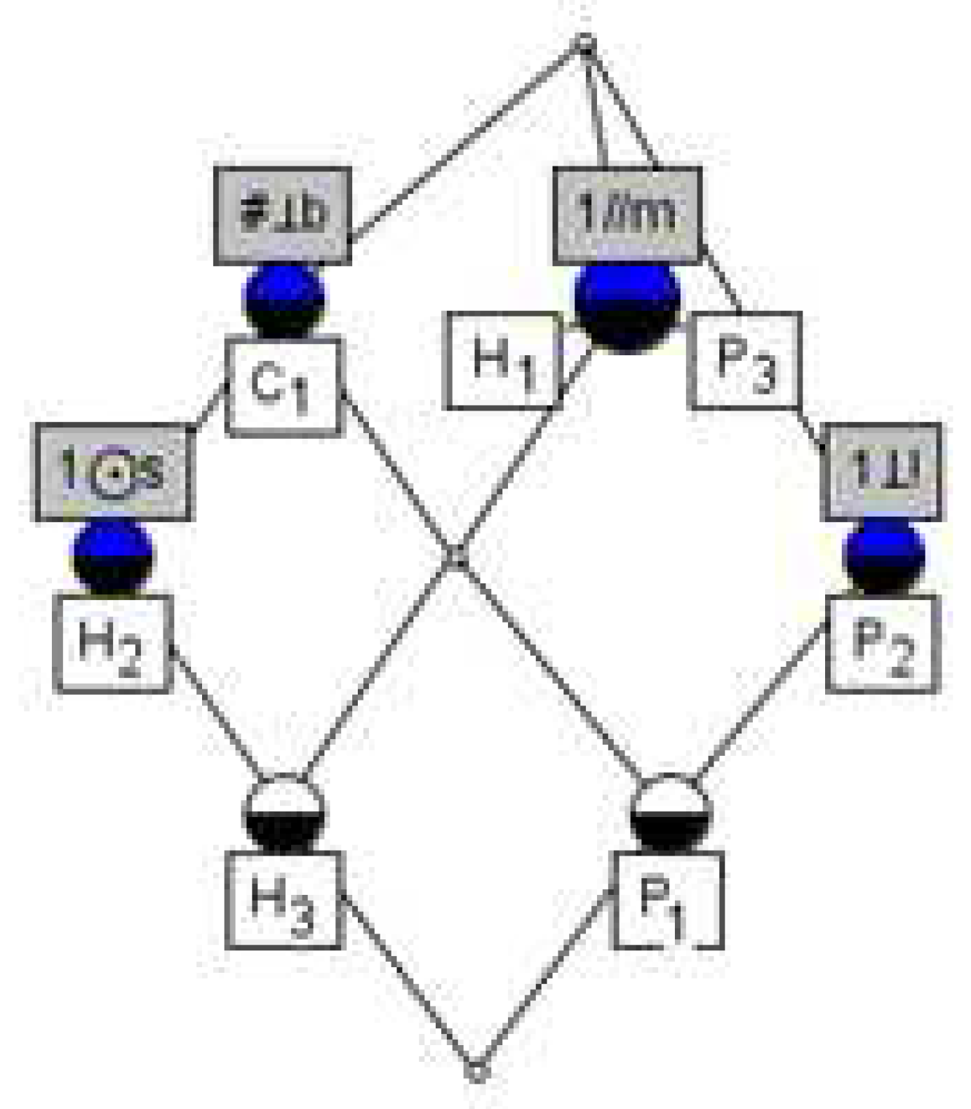
Figure 7.
The formal concept lattice of Table 2.
Figure 7.
The formal concept lattice of Table 2.

Figure 8.
The concept lattice of Table 3.
Figure 8.
The concept lattice of Table 3.

Figure 9.
The concept lattice of Table 4.
Figure 9.
The concept lattice of Table 4.

Figure 10.
The concept lattice of Table 5.
Figure 10.
The concept lattice of Table 5.

Figure 11.
The concept lattice of Table 6.
Figure 11.
The concept lattice of Table 6.

Figure 12.
The concept lattice of Table 7.
Figure 12.
The concept lattice of Table 7.

Figure 13.
The concept lattice of Table 8.
Figure 13.
The concept lattice of Table 8.

Figure 14.
The concept lattice of Table 9.
Figure 14.
The concept lattice of Table 9.


Table 1.
Binary field relations between the functional surfaces.
| Coaxial | Parallel | Vertical | ||||||
|---|---|---|---|---|---|---|---|---|
| Meaning | separate | meet | overlapping | common | amidst | middle | intersect | biased |
| mark | s | m | o | c | d | i | i | b |
| icon |  |  |  |  |  |  |  |  |
Table 2.
The formal context of 3D structure model in Figure 6.
Table 2.
The formal context of 3D structure model in Figure 6.
| 1 | 0 | 0 | 1 | 0 | 0 | 0 | 0 | |
| 1 | 0 | 0 | 1 | 0 | 0 | 0 | 0 | |
| 0 | 0 | 1 | 0 | 0 | 0 | 0 | 0 | |
| 0 | 0 | 1 | 0 | 0 | 0 | 0 | 0 | |
| 0 | 0 | 1 | 0 | 0 | 0 | 0 | 0 | |
| 0 | 0 | 1 | 0 | 0 | 0 | 0 | 0 | |
| 0 | 0 | 1 | 0 | 0 | 0 | 0 | 0 | |
| 1 | 1 | 1 | 0 | 0 | 1 | 0 | 0 | |
| 0 | 1 | 0 | 1 | 1 | 0 | 0 | 0 |
Table 3.
A tabular form, or cross table, with and . The relation I is indicated by the set of crosses in the table.
Table 3.
A tabular form, or cross table, with and . The relation I is indicated by the set of crosses in the table.
| a | b | c | d | e | |
|---|---|---|---|---|---|
| 1 | × | × | |||
| 2 | × | ||||
| 3 | × | × | × | ||
| 4 | × | × | |||
| 5 | × | × | × | × |
Table 4.
A formal context.
| E | F | G | K | L | |
|---|---|---|---|---|---|
| 1 | × | × | |||
| 2 | × | × | × | ||
| 3 | × | × | |||
| 4 | × | × | × | × | |
| 5 | × | ||||
| 6 | × | ||||
| 7 | × | × |
Table 5.
Weight table of single attribute intent.
| A | W |
|---|---|
| E | 0.1 |
| F | 0.2 |
| G | 0.7 |
| K | 0.9 |
| L | 1 |
Table 6.
A formal context of the part.
| 1 | 1 | 1 | 0 | 0 | |
| 0 | 1 | 1 | 0 | 0 | |
| 1 | 0 | 0 | 0 | 0 | |
| H | 0 | 0 | 0 | 0 | 1 |
| 0 | 0 | 1 | 1 | 0 | |
| 0 | 0 | 1 | 1 | 0 | |
| 0 | 1 | 0 | 0 | 1 | |
| 0 | 1 | 0 | 0 | 0 |
Table 7.
A decision formal context.
| a | b | c | d | e | f | g | h | k | |
|---|---|---|---|---|---|---|---|---|---|
| 1 | 0 | 1 | 1 | 1 | 0 | 1 | 0 | 1 | |
| 1 | 0 | 1 | 0 | 0 | 0 | 1 | 0 | 1 | |
| 0 | 1 | 0 | 0 | 1 | 1 | 0 | 1 | 0 | |
| 0 | 1 | 0 | 0 | 1 | 1 | 0 | 1 | 0 | |
| 1 | 0 | 0 | 0 | 0 | 0 | 0 | 0 | 1 | |
| 1 | 1 | 0 | 0 | 1 | 1 | 0 | 1 | 1 |
Table 8.
The value of a double bond set.
| X | B | |
|---|---|---|
| 47/90 | ||
| 1/4 | ||
| 1/2 | ||
| 1 | ||
| 2/3 | ||
| 3/5 | ||
| 2/5 |
Table 9.
The value of a sets of cylinder.
| X | B | |
|---|---|---|
| 1/2 | ||
| 1/3 | ||
| 1/2 | ||
| 1/4 | ||
| 13/36 | ||
| 1/4 | ||
| 1/3 | ||
| 1/3 | ||
| 1/3 | ||
| 1/2 | ||
| 1/3 |
Table 10.
The value of a fork.
| X | B | |
|---|---|---|
| 2/3 | ||
| 5/9 | ||
| 1/4 | ||
| 1/3 | ||
| 3/4 | ||
| 1/2 |
Table 11.
The value of a tray.
| X | B | |
|---|---|---|
| 5/9 | ||
| 2/3 | ||
| 1/2 | ||
| 1/3 | ||
| 2/3 | ||
| 3/4 | ||
| 3/4 | ||
| 2/3 |
Table 12.
The value of a gear unit housing.
| X | B | |
|---|---|---|
| 1361/2160 | ||
| 1/2 | ||
| 1/2 | ||
| 4/9 | ||
| 7/18 | ||
| 2/5 | ||
| 1/4 | ||
| 1/3 | ||
| 1 | ||
| 1/2 | ||
| 1 | ||
| 1/4 | ||
| 3/8 | ||
| 1/4 | ||
| 1/4 |
Table 13.
Important concepts and key structures of the 3D parts structural model.
| Model Name | Important Concept | Key Structure |
|---|---|---|
| [Cow][Cow] | ||
Table 14.
The parts and time consuming that are similar to the model in the model base(I).
| Model | Time (s) | 001 | 002 | 003 | 004 | 005 | 006 | 007 |
|---|---|---|---|---|---|---|---|---|
 | This method 18.137 |  |  |  |  |  |  |  |
| Ref. [7] method 26.334 | | | | | |
Table 15.
The parts and time consuming that are similar to the model in the model base(II).
| Model | Time (s) | 008 | 009 | 010 | 011 | 012 | 013 | 014 |
|---|---|---|---|---|---|---|---|---|
 | This method 31.072 |  |  |  |  |  |  |  |
| Ref. [7] method 38.256 | | | | | |
© 2020 by the authors. Licensee MDPI, Basel, Switzerland. This article is an open access article distributed under the terms and conditions of the Creative Commons Attribution (CC BY) license (http://creativecommons.org/licenses/by/4.0/).
Share and Cite
MDPI and ACS Style
Wu, Q.; Dong, Y.; Xie, L. Finding the Key Structure of Mechanical Parts with Formal Concept Analysis. Information 2020, 11, 116. https://0-doi-org.brum.beds.ac.uk/10.3390/info11020116
AMA Style
Wu Q, Dong Y, Xie L. Finding the Key Structure of Mechanical Parts with Formal Concept Analysis. Information. 2020; 11(2):116. https://0-doi-org.brum.beds.ac.uk/10.3390/info11020116
Chicago/Turabian StyleWu, Qiang, Yan Dong, and Liping Xie. 2020. "Finding the Key Structure of Mechanical Parts with Formal Concept Analysis" Information 11, no. 2: 116. https://0-doi-org.brum.beds.ac.uk/10.3390/info11020116
Note that from the first issue of 2016, this journal uses article numbers instead of page numbers. See further details here.