A Responsible Machine Learning Workflow with Focus on Interpretable Models, Post-hoc Explanation, and Discrimination Testing


Abstract
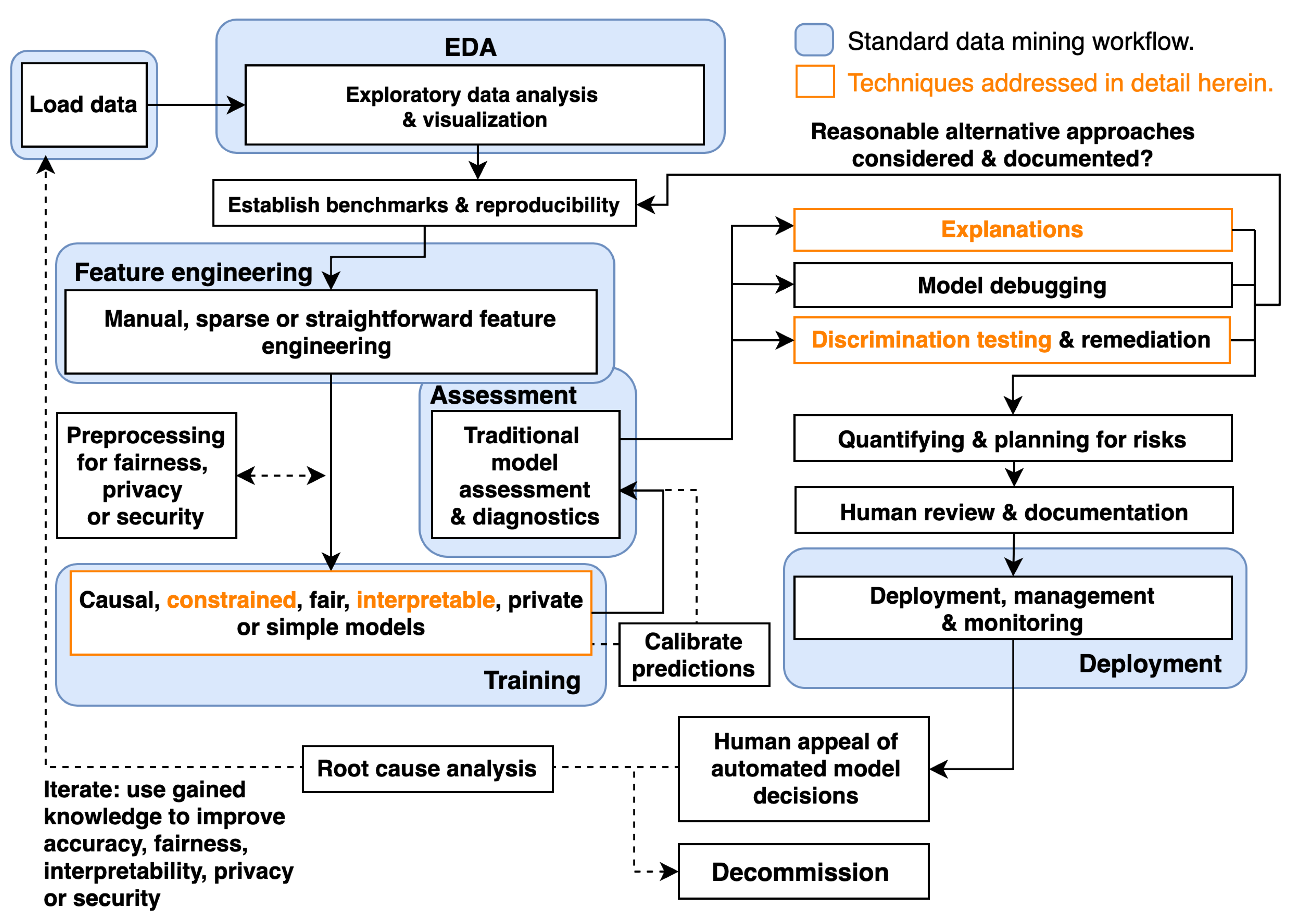
:1. Introduction
2. Materials and Methods
2.1. Simulated Data
2.2. Mortgage Data
2.3. Monotonic Gradient Boosting Machines
2.4. Explainable Neural Networks
2.5. One-Dimensional Partial Dependence and Individual Conditional Expectation
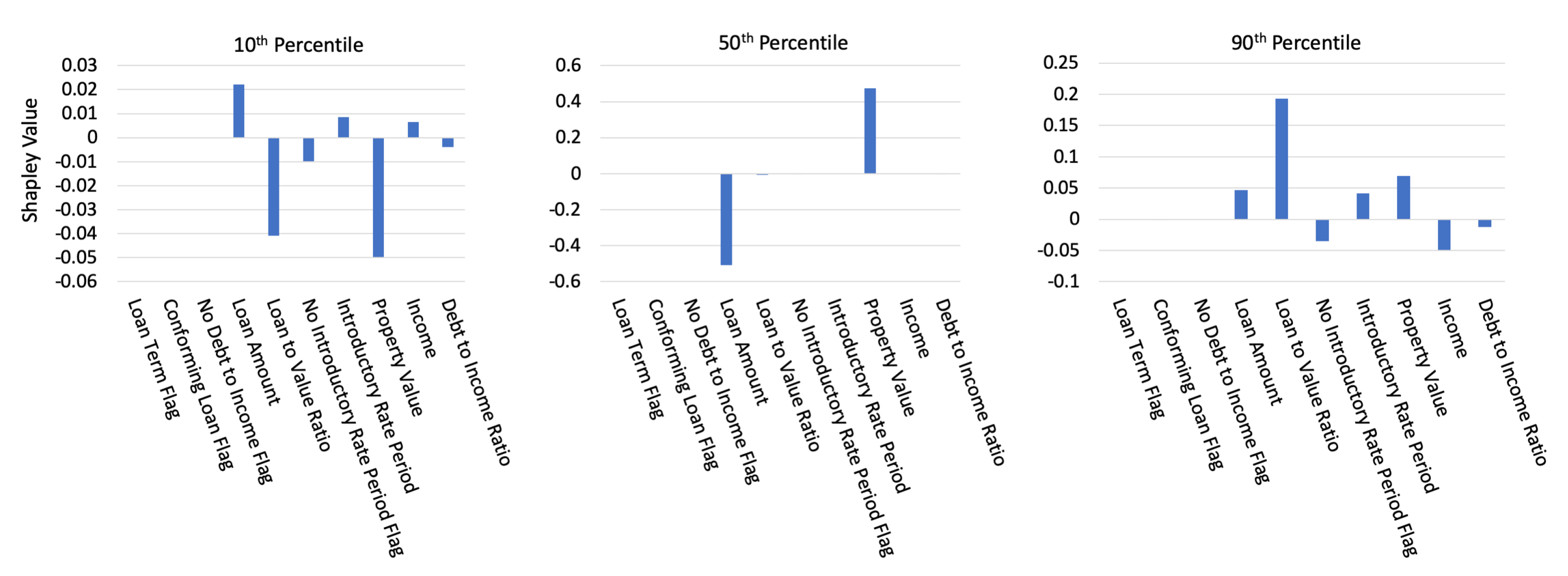
2.6. Shapley Values
2.7. Discrimination Testing Measures
2.8. Software Resources
3. Results
3.1. Simulated Data Results
3.1.1. Constrained vs. Unconstrained Model Fit Assessment
3.1.2. Interpretability Results
3.2. Mortgage Data Results
3.2.1. Constrained vs. Unconstrained Model Fit Assessment
3.2.2. Interpretability and Post-hoc Explanation Results
3.2.3. Discrimination Testing Results
4. Discussion
4.1. The Burgeoning Python Ecosystem for Responsible Machine Learning
4.2. Appeal and Override of Automated Decisions
4.3. Discrimination Testing and Remediation in Practice
4.4. Intersectional and Non-Static Risks in Machine Learning
5. Conclusions
Author Contributions
Funding
Acknowledgments
Conflicts of Interest
Abbreviations
| AI | artificial intelligence |
| AIR | adverse impact ratio |
| ALE | accumulated local effect |
| ANN | artificial neural network |
| APR | annual percentage rate |
| AUC | area under the curve |
| CFPB | Consumer Financial Protection Bureau |
| DI | disparate impact |
| DT | disparate treatment |
| DTI | debt to income |
| EBM or GA2M | explainable boosting machine, i.e., variants GAMs that consider two-way interactions and |
| may incorporate boosting into training | |
| EEOC | Equal Employment Opportunity Commission |
| ECOA | Equal Credit Opportunity Act |
| EDA | exploratory data analysis |
| EU | European Union |
| FCRA | Fair Credit Reporting Act |
| FNR | false negative rate |
| FPR | false positive rate |
| GAM | generalized additive model |
| GBM | gradient boosting machine |
| GDPR | General Data Protection Regulation |
| HMDA | Home Mortgage Disclosure Act |
| ICE | individual conditional expectation |
| LTV | loan to value |
| MCC | Matthews correlation coefficient |
| ME | marginal effect |
| MGBM | monotonic gradient boosting machine |
| ML | machine learning |
| PD | partial dependence |
| RMSE | root mean square error |
| SGD | stochastic gradient descent |
| SHAP | Shapley Additive Explanation |
| SMD | standardized mean difference |
| SR | supervision and regulation |
| US | United States |
| XNN | explainable neural network |
Appendix A. Mortgage Data Details
Appendix B. Selected Algorithmic Details
Appendix B.1. Notation
Appendix B.1.1. Spaces
- Input features come from the set contained in a P-dimensional input space, . An arbitrary, potentially unobserved, or future instance of is denoted , .
- Labels corresponding to instances of come from the set .
- Learned output responses of models are contained in the set .
Appendix B.1.2. Data
- An input dataset is composed of observed instances of the set with a corresponding dataset of labels , observed instances of the set .
- Each i-th observed instance of is denoted as , with corresponding i-th labels in , and corresponding predictions in .
- and consist of N tuples of observed instances: .
- Each j-th input column vector of is denoted as .
Appendix B.1.3. Models
- A type of ML model g, selected from a hypothesis set , is trained to represent an unknown signal-generating function f observed as with labels using a training algorithm : , such that .
- g generates learned output responses on the input dataset , and on the general input space .
- A model to be explained or tested for discrimination is denoted as g.
Appendix B.2. Monotonic Gradient Boosting Machine Details
- For the first and highest split in involving , any resulting in where , is not considered.
- For any subsequent left child node involving , any resulting in where , is not considered.
- Moreover, for any subsequent left child node involving , , are bound by the associated set of node weights, , such that .
- (1) and (2) are also applied to all right child nodes, except that for right child nodes and .
Appendix B.3. Explainable Neural Network Details
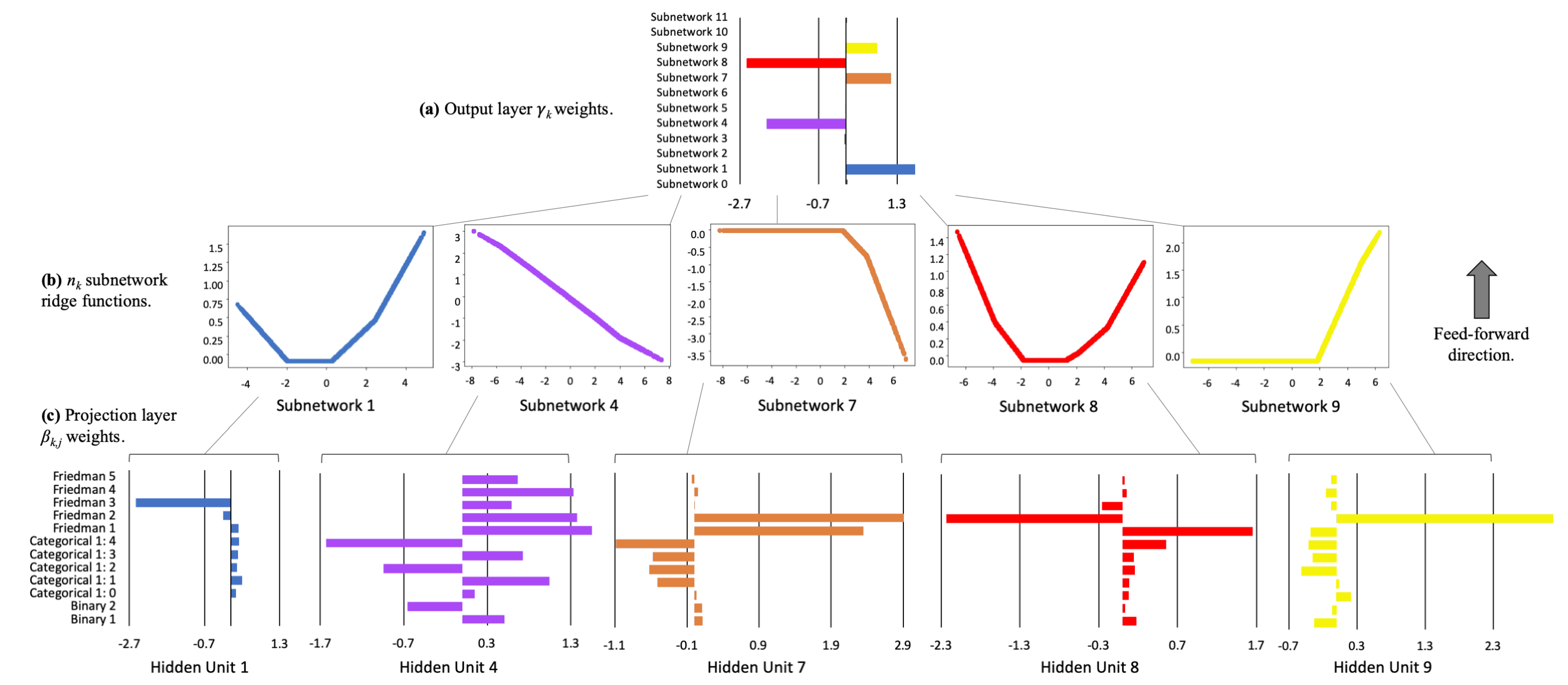
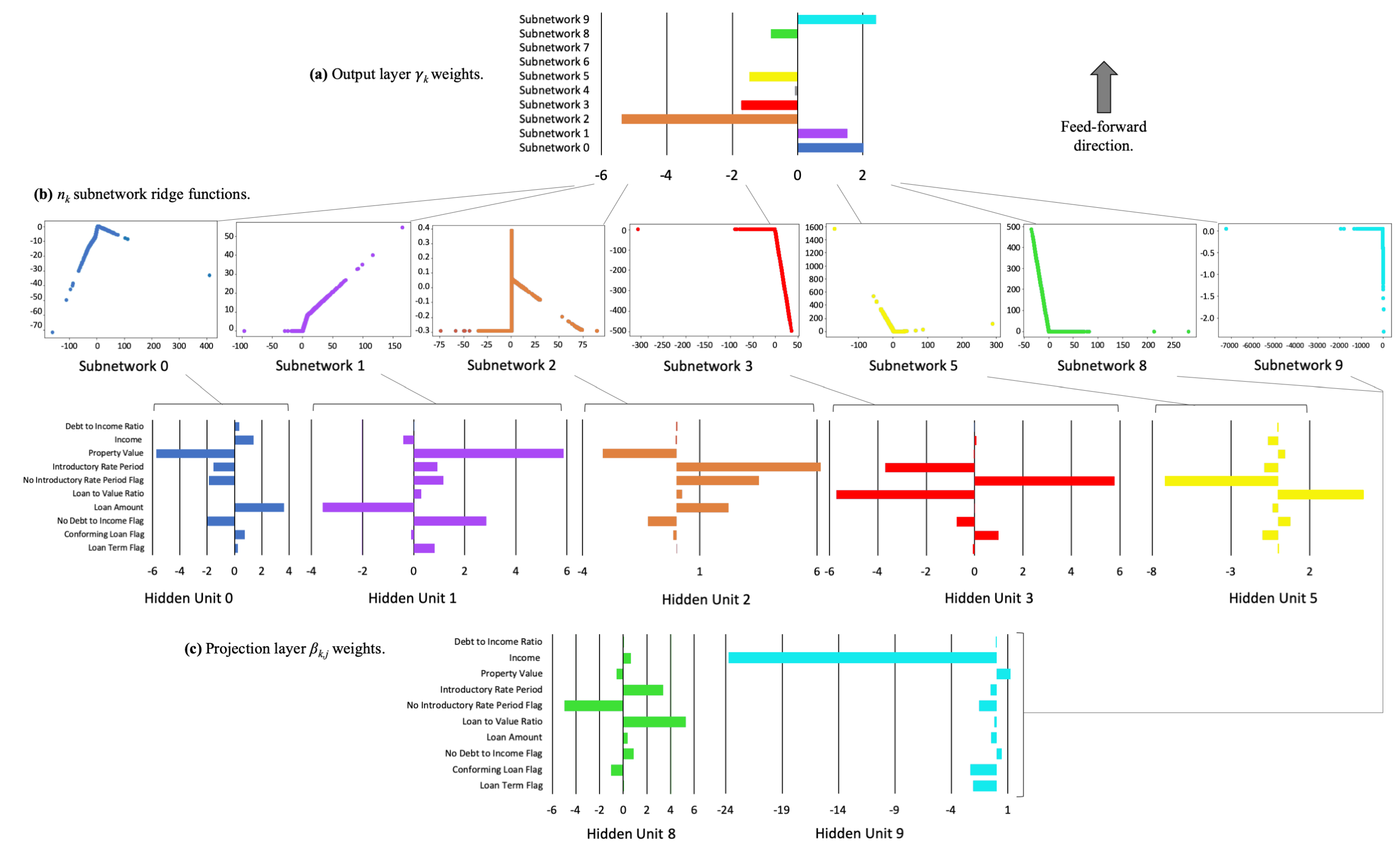
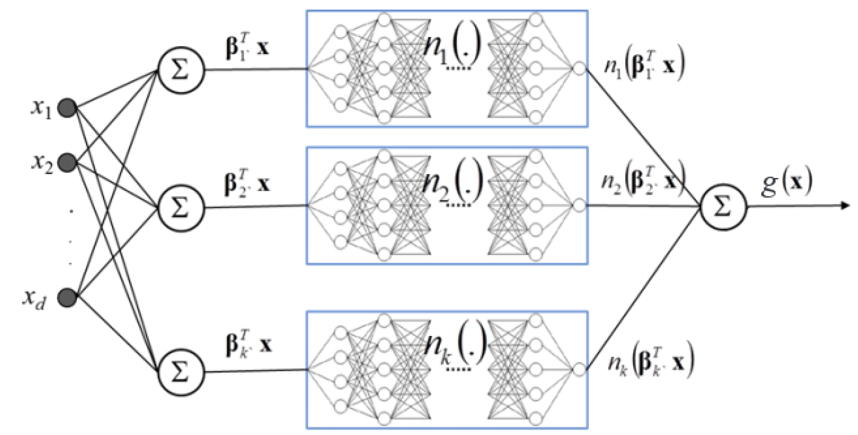
- The first and deepest meta-layer, composed of K linear hidden units (see Equation (3)), which should learn higher magnitude weights for each important input, , is known as the projection layer. It is fully connected to each input . Each hidden unit in the projection layer may optionally include a bias term.
- The second meta-layer contains K hidden and separate ridge functions, or subnetworks. Each is a neural network itself, which can be parametrized to suit a given modeling task. To facilitate direct interpretation and visualization, the input to each subnetwork is the 1-dimensional output of its associated projection layer hidden unit. Each can contain several bias terms.
- The output meta-layer, called the combination layer, is an output neuron comprised of a global bias term, , and the K weighted 1-dimensional outputs of each subnetwork, . Again, each subnetwork output into the combination layer is restricted to 1-dimension for interpretation and visualization purposes.

Appendix B.4. One-dimensional Partial Dependence and Individual Conditional Expectation Details
Appendix B.5. Shapley Value Details
Appendix C. Types of Machine Learning Discrimination in US Legal and Regulatory Settings
Appendix D. Practical vs. Statistical Significance for Discrimination Testing
Appendix E. Additional Simulated Data Results
Appendix E.1. Interpretability and Post-hoc Explanation Results


Appendix E.2. Discrimination Testing Results

| Class | Model | Accuracy↑ | FNR↓ | |
| Protected 1 | 3057 | 0.770 0.771 | 0.401 0.357 | |
| Control 1 | 16,943 | 0.739 0.756 | 0.378 0.314 | |
| Protected 2 | 9916 | 0.758 0.762 | 0.331 0.302 | |
| Control 2 | 10,084 | 0.729 0.756 | 0.420 0.332 |
| Model | Protected Class | Control Class | AIR↑ | ME↓ | SMD↓ | FNR Ratio↓ |
| 1 2 | 1 2 | 0.752 1.10 | 9.7% −3.6% | −0.206 0.106 | 1.06 0.788 | |
| 1 2 | 1 2 | 0.727 0.976 | 12.0% 1.0% | −0.274 0.001 | 1.13 0.907 |
Appendix F. Discrimination Testing and Cutoff Selection
Appendix G. Recent Fairness Techniques in US Legal and Regulatory Settings
References
- Rudin, C. Please Stop Explaining Black Box Models for High Stakes Decisions and Use Interpretable Models Instead. arXiv 2018, arXiv:1811.10154. Available online: https://arxiv.org/pdf/1811.10154.pdf (accessed on 26 February 2020).
- Feldman, M.; Friedler, S.A.; Moeller, J.; Scheidegger, C.; Venkatasubramanian, S. Certifying and Removing Disparate Impact. In Proceedings of the 21st ACM SIGKDD International Conference on Knowledge Discovery and Data Mining, Sydney, Australia, 10–13 August 2015; pp. 259–268. Available online: https://arxiv.org/pdf/1412.3756.pdf (accessed on 26 February 2020).
- Dwork, C.; Hardt, M.; Pitassi, T.; Reingold, O.; Zemel, R. Fairness Through Awareness. In Proceedings of the 3rd Innovations in Theoretical Computer Science Conference, Cambridge, MA, USA, 8–10 January 2012; pp. 214–226. Available online: https://arxiv.org/pdf/1104.3913.pdf (accessed on 26 February 2020).
- Buolamwini, J.; Gebru, T. Gender Shades: Intersectional Accuracy Disparities in Commercial Gender Classification. In Proceedings of the Conference on Fairness, Accountability and Transparency, New York, NY, USA, 23–24 February 2018; pp. 77–91. Available online: http://proceedings.mlr.press/v81/buolamwini18a/buolamwini18a.pdf (accessed on 26 February 2020).
- Barreno, M.; Nelson, B.; Joseph, A.D.; Tygar, J. The Security of Machine Learning. Mach. Learn. 2010, 81, 121–148. Available online: http://people.ischool.berkeley.edu/~tygar/papers/SML/sec_mach_learn_journal.pdf (accessed on 26 February 2020). [CrossRef] [Green Version]
- Tramèr, F.; Zhang, F.; Juels, A.; Reiter, M.K.; Ristenpart, T. Stealing Machine Learning Models via Prediction APIs. In Proceedings of the 25th USENIX Security Symposium, Austin, TX, USA, 10–12 August 2016; pp. 601–618. Available online: https://www.usenix.org/system/files/conference/usenixsecurity16/sec16_paper_tramer.pdf (accessed on 26 February 2020).
- Shokri, R.; Stronati, M.; Song, C.; Shmatikov, V. Membership Inference Attacks Against Machine Learning Models. In Proceedings of the 2017 IEEE Symposium on Security and Privacy (SP), San Jose, CA, USA, 25 May 2017; pp. 3–18. Available online: https://arxiv.org/pdf/1610.05820.pdf (accessed on 26 February 2020).
- Shokri, R.; Strobel, M.; Zick, Y. Privacy Risks of Explaining Machine Learning Models. arXiv 2019, arXiv:1907.00164. Available online: https://arxiv.org/pdf/1907.00164.pdf (accessed on 26 February 2020).
- Williams, M. Interpretability; Fast Forward Labs: Brooklyn, NY, USA, 2017; Available online: https://www.cloudera.com/products/fast-forward-labs-research.html (accessed on 26 February 2020).
- Friedman, J.H. A Tree-structured Approach to Nonparametric Multiple Regression. In Smoothing Techniques for Curve Estimation; Springer: Berlin/Heidelberg, Germany, 1979; pp. 5–22. Available online: http://inspirehep.net/record/140963/files/slac-pub-2336.pdf (accessed on 28 February 2020).
- Friedman, J.H. Multivariate Adaptive Regression Splines. Ann. Stat. 1991, 19, 1–67. Available online: https://projecteuclid.org/download/pdf_1/euclid.aos/1176347963 (accessed on 28 February 2020). [CrossRef]
- Mortgage Data (HMDA). Available online: https://www.consumerfinance.gov/data-research/hmda/ (accessed on 24 February 2020).
- Friedman, J.H. Greedy Function Approximation: a Gradient Boosting Machine. Ann. Stat. 2001, 1189–1232. Available online: https://statweb.stanford.edu/~jhf/ftp/trebst.pdf (accessed on 28 February 2020).
- Friedman, J.H.; Hastie, T.; Tibshirani, R. The Elements of Statistical Learning; Springer: New York, NY, USA, 2001; Available online: https://web.stanford.edu/~hastie/ElemStatLearn/printings/ESLII_print12.pdf (accessed on 26 February 2020).
- Recht, B.; Re, C.; Wright, S.; Niu, F. HOGWILD: A Lock-free Approach to Parallelizing Stochastic Gradient Descent. Available online: https://papers.nips.cc/paper/4390-hogwild-a-lock-free-approach-to-parallelizing-stochastic-gradient-descent.pdf (accessed on 26 February 2020).
- Hinton, G.E.; Srivastava, N.; Krizhevsky, A.; Sutskever, I.; Salakhutdinov, R.R. Improving Neural Networks by Preventing Co-adaptation of Feature Detectors. arXiv 2012, arXiv:1207.0580. Available online: https://arxiv.org/pdf/1207.0580.pdf (accessed on 26 February 2020).
- Sutskever, I.; Martens, J.; Dahl, G.; Hinton, G. On the Importance of Initialization and Momentum in Deep Learning. In Proceedings of the International Conference on Machine Learning, Atlanta, GA, USA, 16–21 June 2013; pp. 1139–1147. Available online: http://proceedings.mlr.press/v28/sutskever13.pdf (accessed on 26 February 2020).
- Zeiler, M.D. ADADELTA: An Adaptive Learning Rate Method. arXiv 2012, arXiv:1212.5701. Available online: https://arxiv.org/pdf/1212.5701.pdf (accessed on 26 February 2020).
- Aïvodji, U.; Arai, H.; Fortineau, O.; Gambs, S.; Hara, S.; Tapp, A. Fairwashing: The Risk of Rationalization. arXiv 2019, arXiv:1901.09749. Available online: https://arxiv.org/pdf/1901.09749.pdf (accessed on 26 February 2020).
- Slack, D.; Hilgard, S.; Jia, E.; Singh, S.; Lakkaraju, H. Fooling LIME and SHAP: Adversarial Attacks on Post-hoc Explanation Methods. arXiv 2019, arXiv:1911.02508. Available online: https://arxiv.org/pdf/1911.02508.pdf (accessed on 26 February 2020).
- Vaughan, J.; Sudjianto, A.; Brahimi, E.; Chen, J.; Nair, V.N. Explainable Neural Networks Based on Additive Index Models. arXiv 2018, arXiv:1806.01933. Available online: https://arxiv.org/pdf/1806.01933.pdf (accessed on 26 February 2020).
- Yang, Z.; Zhang, A.; Sudjianto, A. Enhancing Explainability of Neural Networks Through Architecture Constraints. arXiv 2019, arXiv:1901.03838. Available online: https://arxiv.org/pdf/1901.03838.pdf (accessed on 26 February 2020).
- Goldstein, A.; Kapelner, A.; Bleich, J.; Pitkin, E. Peeking Inside the Black Box: Visualizing Statistical Learning with Plots of Individual Conditional Expectation. J. Comput. Graph. Stat. 2015, 24. Available online: https://arxiv.org/pdf/1309.6392.pdf (accessed on 26 February 2020). [CrossRef]
- Lundberg, S.M.; Lee, S.I. A Unified Approach to Interpreting Model Predictions. In Advances in Neural Information Processing Systems (NIPS); Guyon, I., Luxburg, U.V., Bengio, S., Wallach, H., Fergus, R., Vishwanathan, S., Garnett, R., Eds.; Curran Associates, Inc.: Red Hook, NY, USA, 2017; pp. 4765–4774. Available online: http://papers.nips.cc/paper/7062-a-unified-approach-to-interpreting-model-predictions.pdf (accessed on 26 February 2020).
- Lundberg, S.M.; Erion, G.G.; Lee, S.I. Consistent Individualized Feature Attribution for Tree Ensembles. In Proceedings of the 2017 ICML Workshop on Human Interpretability in Machine Learning (WHI 2017), Sydney, Australia, 10 August 2017; pp. 15–21. Available online: https://openreview.net/pdf?id=ByTKSo-m- (accessed on 26 February 2020).
- Cohen, J. Statistical Power Analysis for the Behavioral Sciences; Lawrence Erlbaum Associates: Mahwah, NJ, USA, 1988; Available online: http://www.utstat.toronto.edu/~brunner/oldclass/378f16/readings/CohenPower.pdf (accessed on 26 February 2020).
- Cohen, J. A Power Primer. Psychol. Bull. 1992, 112, 155. Available online: https://www.ime.usp.br/~abe/lista/pdfn45sGokvRe.pdf (accessed on 26 February 2020). [CrossRef]
- Zafar, M.B.; Valera, I.; Gomez Rodriguez, M.; Gummadi, K.P. Fairness Beyond Disparate Treatment & Disparate Impact: Learning Classification Without Disparate Mistreatment. In Proceedings of the 26th International Conference onWorldWideWeb, Perth, Australia, 3–7 April 2017; pp. 1171–1180. Available online: https://arxiv.org/pdf/1610.08452.pdf (accessed on 26 February 2020).
- Lou, Y.; Caruana, R.; Gehrke, J.; Hooker, G. Accurate Intelligible Models with Pairwise Interactions. In Proceedings of the 19th ACM SIGKDD International Conference on Knowledge Discovery and Data Mining, Chicago, IL, USA, 11–14 August 2013; pp. 623–631. Available online: http://citeseerx.ist.psu.edu/viewdoc/download?doi=10.1.1.352.7682&rep=rep1&type=pdf (accessed on 26 February 2020).
- Apley, D.W. Visualizing the Effects of Predictor Variables in Black Box Supervised Learning Models. arXiv 2016, arXiv:1612.08468. Available online: https://arxiv.org/pdf/1612.08468.pdf (accessed on 26 February 2020).
- Shapley, L.S.; Roth, A.E. The Shapley value: Essays in Honor of Lloyd S. Shapley; Cambridge University Press: Cambridge, UK, 1988; Available online: http://www.library.fa.ru/files/Roth2.pdf (accessed on 26 February 2020).
- Hall, P. On the Art and Science of Machine Learning Explanations. Available online: https://arxiv.org/pdf/1810.02909.pdf (accessed on 26 February 2020).
- Molnar, C. Interpretable Machine Learning. Available online: https://christophm.github.io/interpretableml-book/ (accessed on 26 February 2020).
- Hu, X.; Rudin, C.; Seltzer, M. Optimal Sparse Decision Trees. arXiv 2019, arXiv:1904.12847. Available online: https://arxiv.org/pdf/1904.12847.pdf (accessed on 26 February 2020).
- Chen, C.; Li, O.; Barnett, A.; Su, J.; Rudin, C. This Looks Like That: Deep Learning for Interpretable Image Recognition. Proceedings of Neural Information Processing Systems (NeurIPS), Vancouver, BC, Canada, 8–14 December 2019; Available online: https://arxiv.org/pdf/1806.10574.pdf (accessed on 26 February 2020).
- Friedman, J.H.; Popescu, B.E. Predictive Learning Via Rule Ensembles. Ann. Appl. Stat. 2008, 2, 916–954. Available online: https://projecteuclid.org/download/pdfview_1/euclid.aoas/1223908046 (accessed on 26 February 2020). [CrossRef]
- Gupta, M.; Cotter, A.; Pfeifer, J.; Voevodski, K.; Canini, K.; Mangylov, A.; Moczydlowski, W.; Van Esbroeck, A. Monotonic Calibrated Interpolated Lookup Tables. J. Mach. Learn. Res. 2016, 17, 3790–3836. Available online: http://www.jmlr.org/papers/volume17/15-243/15-243.pdf (accessed on 26 February 2020).
- Wilkinson, L. Visualizing Big Data Outliers through Distributed Aggregation. IEEE Trans. Vis. Comput. Graph. 2018. Available online: https://www.cs.uic.edu/~wilkinson/Publications/outliers.pdf (accessed on 26 February 2020).
- Udell, M.; Horn, C.; Zadeh, R.; Boyd, S. Generalized Low Rank Models. Found. Trends® Mach. Learn. 2016, 9, 1–118. Available online: https://www.nowpublishers.com/article/Details/MAL-055 (accessed on 26 February 2020). [CrossRef]
- Holohan, N.; Braghin, S.; Mac Aonghusa, P.; Levacher, K. Diffprivlib: The IBM Differential Privacy Library. arXiv 2019, arXiv:1907.02444. Available online: https://arxiv.org/pdf/1907.02444.pdf (accessed on 26 February 2020).
- Ji, Z.; Lipton, Z.C.; Elkan, C. Differential Privacy and Machine Learning: A Survey and Review. arXiv 2014, arXiv:1412.7584. Available online: https://arxiv.org/pdf/1412.7584.pdf (accessed on 26 February 2020).
- Papernot, N.; Song, S.; Mironov, I.; Raghunathan, A.; Talwar, K.; Erlingsson, Ú. Scalable Private Learning with PATE. arXiv 2018, arXiv:1802.08908. Available online: https://arxiv.org/pdf/1802.08908.pdf (accessed on 26 February 2020).
- Abadi, M.; Chu, A.; Goodfellow, I.; McMahan, H.B.; Mironov, I.; Talwar, K.; Zhang, L. Deep Learning with Differential Privacy. In Proceedings of the 2016 ACM SIGSAC Conference on Computer and Communications Security, Vienna, Austria, 24–28 October 2016; pp. 308–318. Available online: https://arxiv.org/pdf/1607.00133.pdf (accessed on 26 February 2020).
- Pearl, J.; Mackenzie, D. The Book of Why: The New Science of Cause and Effect. Available online: http://cdar.berkeley.edu/wp-content/uploads/2017/04/Lisa-Goldberg-reviews-The-Book-of-Why.pdf (accessed on 26 February 2020).
- Wachter, S.; Mittelstadt, B.; Russell, C. Counterfactual Explanations without Opening the Black Box: Automated Decisions and the GPDR. Harv. JL Tech. 2017, 31, 841. Available online: https://arxiv.org/pdf/1711.00399.pdf (accessed on 26 February 2020). [CrossRef] [Green Version]
- Ancona, M.; Ceolini, E.; Oztireli, C.; Gross, M. Towards Better Understanding of Gradient-based Attribution Methods for Deep Neural Networks. In Proceedings of the 6th International Conference on Learning Representations (ICLR 2018), Vancouver, BC, Canada, 30 April–3 May 2018; Available online: https://www.research-collection.ethz.ch/bitstream/handle/20.500.11850/249929/Flow_ICLR_2018.pdf (accessed on 26 February 2020).
- Wallace, E.; Tuyls, J.; Wang, J.; Subramanian, S.; Gardner, M.; Singh, S. AllenNLP Interpret: A Framework for Explaining Predictions of NLP Models. arXiv 2019, arXiv:1909.09251. Available online: https://arxiv.org/pdf/1909.09251.pdf (accessed on 26 February 2020).
- Kamiran, F.; Calders, T. Data Preprocessing Techniques for Classification Without Discrimination. Knowl. Inf. Syst. 2012, 33, 1–33. Available online: https://bit.ly/2lH95lQ (accessed on 26 February 2020). [CrossRef] [Green Version]
- Zhang, B.H.; Lemoine, B.; Mitchell, M. Mitigating Unwanted Biases with Adversarial Learning. In Proceedings of the 2018 AAAI/ACM Conference on AI, Ethics, and Society, New Orleans, LA, USA, 2–3 February 2018; pp. 335–340. Available online: https://arxiv.org/pdf/1801.07593.pdf (accessed on 26 February 2020).
- Zemel, R.; Wu, Y.; Swersky, K.; Pitassi, T.; Dwork, C. Learning Fair Representations. In Proceedings of the International Conference on Machine Learning, Atlanta, GA, USA, 16–21 June 2013; pp. 325–333. Available online: http://proceedings.mlr.press/v28/zemel13.pdf (accessed on 26 February 2020).
- Kamiran, F.; Karim, A.; Zhang, X. Decision Theory for Discrimination-aware Classification. In Proceedings of the 2012 IEEE 12th International Conference on Data Mining, Brussels, Belgium, 10 December 2012; p. 924. Available online: http://citeseerx.ist.psu.edu/viewdoc/download?doi=10.1.1.722.3030&rep=rep1&type=pdf (accessed on 26 February 2020).
- Rauber, J.; Brendel, W.; Bethge, M. Foolbox: A Python Toolbox to Benchmark the Robustness of Machine Learning Models. arXiv 2017, arXiv:1707.04131. Available online: https://arxiv.org/pdf/1707.04131.pdf (accessed on 26 February 2020).
- Papernot, N.; Faghri, F.; Carlini, N.; Goodfellow, I.; Feinman, R.; Kurakin, A.; Xie, C.; Sharma, Y.; Brown, T.; Roy, A.; et al. Technical Report on the CleverHans v2.1.0 Adversarial Examples Library. arXiv 2018, arXiv:1610.00768. Available online: https://arxiv.org/pdf/1610.00768.pdf (accessed on 26 February 2020).
- Amershi, S.; Chickering, M.; Drucker, S.M.; Lee, B.; Simard, P.; Suh, J. Modeltracker: Redesigning Performance Analysis Tools for Machine Learning. In Proceedings of the 33rd Annual ACM Conference on Human Factors in Computing Systems, Seoul, Korea, 18–23 April 2015; pp. 337–346. Available online: https://www.microsoft.com/en-us/research/wp-content/uploads/2016/02/amershi.CHI2015.ModelTracker.pdf (accessed on 26 February 2020).
- Papernot, N. A Marauder’s Map of Security and Privacy in Machine Learning: An overview of current and future research directions for making machine learning secure and private. In Proceedings of the 11th ACM Workshop on Artificial Intelligence and Security, Toronto, ON, Canada, 19 October 2018; Available online: https://arxiv.org/pdf/1811.01134.pdf (accessed on 26 February 2020).
- Mitchell, M.; Wu, S.; Zaldivar, A.; Barnes, P.; Vasserman, L.; Hutchinson, B.; Spitzer, E.; Raji, I.D.; Gebru, T. Model Cards for Model Reporting. In Proceedings of the Conference on Fairness, Accountability, and Transparency, Atlanta, GA, USA, 29–31 January 2019; pp. 220–229. Available online: https://arxiv.org/pdf/1810.03993.pdf (accessed on 26 February 2020).
- Bracke, P.; Datta, A.; Jung, C.; Sen, S. Machine Learning Explainability in Finance: An Application to Default Risk Analysis. 2019. Available online: https://0-www-bankofengland-co-uk.brum.beds.ac.uk/-/media/boe/files/working-paper/2019/machine-learning-explainability-in-finance-an-application-to-default-risk-analysis.pdf (accessed on 26 February 2020).
- Friedler, S.A.; Scheidegger, C.; Venkatasubramanian, S.; Choudhary, S.; Hamilton, E.P.; Roth, D. A Comparative Study of Fairness-enhancing Interventions in Machine Learning. In Proceedings of the Conference on Fairness, Accountability, and Transparency, Atlanta, GA, USA, 29–31 January 2019; pp. 329–338. Available online: https://arxiv.org/pdf/1802.04422.pdf (accessed on 26 February 2020).
- Schmidt, N.; Stephens, B. An Introduction to Artificial Intelligence and Solutions to the Problems of Algorithmic Discrimination. Conf. Consum. Financ. Law Q. Rep. 2019, 73, 130–144. Available online: https://arxiv.org/pdf/1911.05755.pdf (accessed on 26 February 2020).
- Hoare, C.A.R. The 1980 ACM Turing Award Lecture. Communications 1981. Available online: http://www.cs.fsu.edu/~engelen/courses/COP4610/hoare.pdf (accessed on 26 February 2020).


| Model | Accuracy ↑ | AUC ↑ | F1 ↑ | Logloss ↓ | MCC ↑ | RMSE ↓ | Sensitivity ↑ | Specificity ↑ |
|---|---|---|---|---|---|---|---|---|
| 0.757 | 0.847 | 0.779 | 0.486 | 0.525 | 0.400 | 0.858 | 0.657 | |
| 0.744 | 0.842 | 0.771 | 0.502 | 0.504 | 0.407 | 0.864 | 0.625 | |
| 0.757 | 0.850 | 0.779 | 0.480 | 0.525 | 0.398 | 0.858 | 0.657 | |
| 0.758 | 0.851 | 0.781 | 0.479 | 0.528 | 0.397 | 0.867 | 0.648 |
| Model | Accuracy ↑ | AUC ↑ | F1 ↑ | Logloss ↓ | MCC ↑ | RMSE ↓ | Sensitivity ↑ | Specificity ↑ |
|---|---|---|---|---|---|---|---|---|
| 0.795 | 0.828 | 0.376 | 0.252 | 0.314 | 0.276 | 0.634 | 0.813 | |
| 0.765 | 0.814 | 0.362 | 0.259 | 0.305 | 0.278 | 0.684 | 0.773 | |
| 0.865 | 0.871 | 0.474 | 0.231 | 0.418 | 0.262 | 0.624 | 0.891 | |
| 0.869 | 0.868 | 0.468 | 0.233 | 0.409 | 0.263 | 0.594 | 0.898 |
| Class | Model | Accuracy↑ | FPR↓ | |
| Black | 2608 | 0.654 0.702 | 0.315 0.295 | |
| White | 28,361 | 0.817 0.857 | 0.150 0.120 | |
| Female | 8301 | 0.768 0.822 | 0.208 0.158 | |
| Male | 13,166 | 0.785 0.847 | 0.182 0.131 |
| Model | Protected Class | Control Class | AIR↑ | ME↓ | SMD↓ | FPR Ratio↓ |
| Black Female | White Male | 0.776 0.948 | 18.3% 4.1% | 0.628 0.084 | 2.10 1.15 | |
| Black Female | White Male | 0.743 0.955 | 21.4% 3.6% | 0.621 0.105 | 2.45 1.21 |
© 2020 by the authors. Licensee MDPI, Basel, Switzerland. This article is an open access article distributed under the terms and conditions of the Creative Commons Attribution (CC BY) license (http://creativecommons.org/licenses/by/4.0/).
Share and Cite
Gill, N.; Hall, P.; Montgomery, K.; Schmidt, N. A Responsible Machine Learning Workflow with Focus on Interpretable Models, Post-hoc Explanation, and Discrimination Testing. Information 2020, 11, 137. https://0-doi-org.brum.beds.ac.uk/10.3390/info11030137
Gill N, Hall P, Montgomery K, Schmidt N. A Responsible Machine Learning Workflow with Focus on Interpretable Models, Post-hoc Explanation, and Discrimination Testing. Information. 2020; 11(3):137. https://0-doi-org.brum.beds.ac.uk/10.3390/info11030137
Chicago/Turabian StyleGill, Navdeep, Patrick Hall, Kim Montgomery, and Nicholas Schmidt. 2020. "A Responsible Machine Learning Workflow with Focus on Interpretable Models, Post-hoc Explanation, and Discrimination Testing" Information 11, no. 3: 137. https://0-doi-org.brum.beds.ac.uk/10.3390/info11030137