A Multi-Task Framework for Action Prediction

School of Computer Science, Shenyang Aerospace University, Shenyang 110136, China
*
Authors to whom correspondence should be addressed.
Information 2020, 11(3), 158; https://0-doi-org.brum.beds.ac.uk/10.3390/info11030158
Submission received: 23 January 2020
/
Revised: 27 February 2020
/
Accepted: 6 March 2020
/
Published: 16 March 2020
Abstract
:Predicting the categories of actions in partially observed videos is a challenging task in the computer vision field. The temporal progress of an ongoing action is of great importance for action prediction, since actions can present different characteristics at different temporal stages. To this end, we propose a novel multi-task deep forest framework, which treats temporal progress analysis as a relevant task to action prediction and takes advantage of observation ratio labels of incomplete videos during training. The proposed multi-task deep forest is a cascade structure of random forests and multi-task random forests. Unlike the traditional single-task random forests, multi-task random forests are built upon incomplete training videos annotated with action labels as well as temporal progress labels. Meanwhile, incorporating both random forests and multi-task random forests can increase the diversity of classifiers and improve the discriminative power of the multi-task deep forest. Experiments on the UT-Interaction and the BIT-Interaction datasets demonstrate the effectiveness of the proposed multi-task deep forest.
1. Introduction
During the past decade, activity prediction has been attracting increasing interest [1,2,3,4], motivated by many potential applications in video surveillance, auto driving, and elderly care. Action prediction takes partially observed videos as input and makes a decision before an action is fully executed. Similar to the human cognitive processes, action prediction methods establish the relationship between the partial observations and action categories by taking advantage of the prior knowledge. For example, it is difficult for a man who has never watched a fencing competition to infer the activity of a fencing athlete. Nevertheless, after watching several competitions, he can tell that the athlete is about to do fencing when the athlete is unsheathing the sword.
Action prediction is an important task related to action recognition [5,6,7] that classifies an action into a certain category after capturing the complete observations. It is evident that predicting actions with incomplete videos is more challenging compared with recognizing actions with full videos. Particularly, an ongoing action can present different motion patterns with sequentially arrived observations, thus the temporal progress of ongoing actions is of great importance for action prediction. However, temporal progress of actions in an input incomplete video is not available during testing.
To overcome the above problem, this paper treats action prediction and temporal progress analysis as two relevant tasks and incorporates them in a multi-task learning framework. Although temporal progress of actions in testing videos cannot be directly observed, we can benefit from the observation ratios of incomplete training videos. The observation ratio represents the proportion of frames that have been observed currently, and can be calculated through dividing the number of frames in an incomplete video by the total number of frames in the corresponding complete videos. It indicates the temporal progress of a training video and can offer important clues for action prediction.
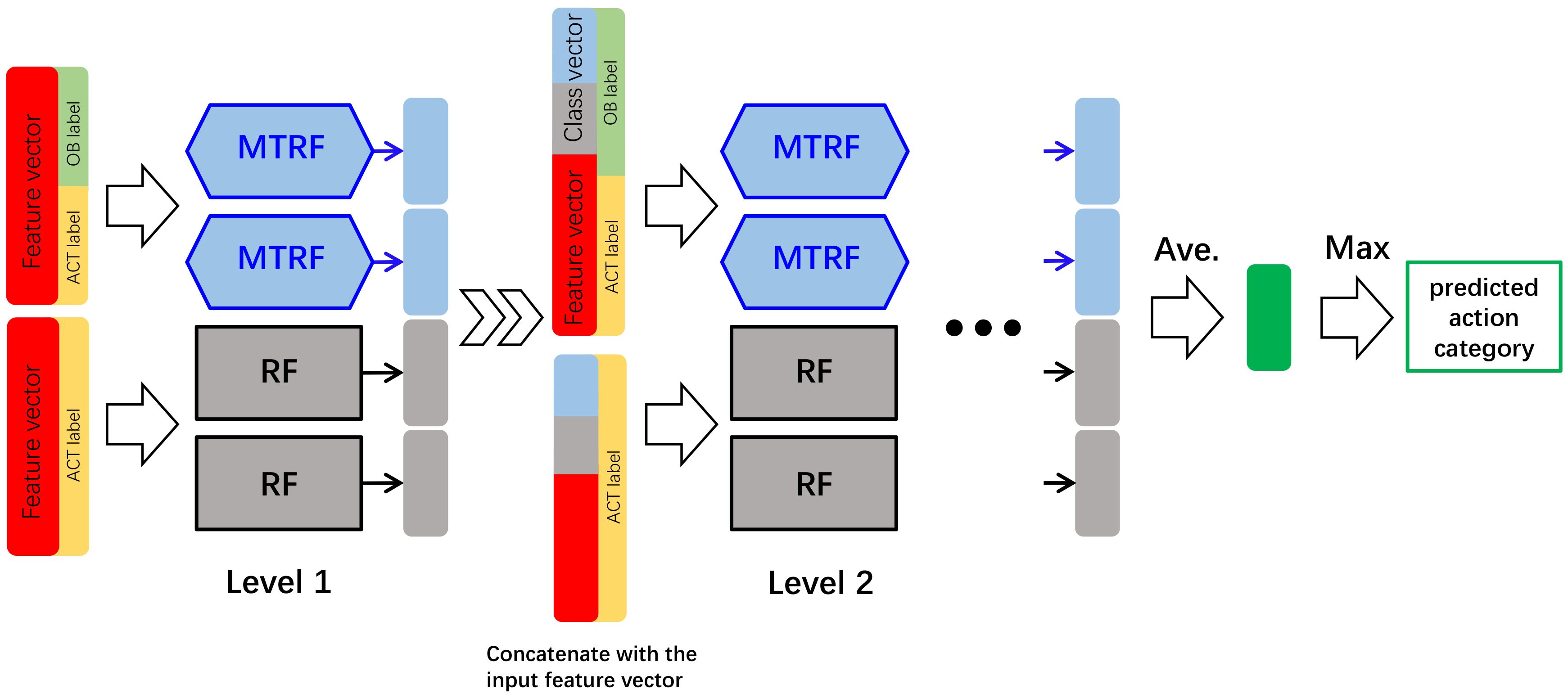
We present a novel Multi-Task Deep Forest (MTDF) framework inspired by the success of gcForest [8]. As shown in Figure 1, the proposed MTDF is a cascade structure of single-task Random Forests (RF) [9] and Multi-Task Random Forests (MTRF). Each level of the cascade exploits two RFs and two MTRFs to learn mid-level features of an input incomplete video. The mid-level features and the original video feature are concatenated to obtain an augmented representation, which is the input of the next level. The final decision of the action category is made upon the mid-level features of the last level. In the proposed MTDF, two kinds of forests (i.e., RF and MTRF) are employed to enhance the diversity so that the ensemble of multiple forests can learn discriminative mid-level features better. Unlike the traditional single-task RF, our MTRF consists of multiple multi-task decision trees that are built upon samples annotated with both action labels and observation ratio labels indicating the temporal progress of actions. A multi-task decision tree jointly deals with the action prediction task and the temporal progress recognition task. Specifically, in the construction of a multi-task decision tree, one type of labels is randomly selected for node split.
The structure of the paper is as follows. A brief summary of the relevant literature is presented in Section 2. Section 3 gives a fine description of the proposed multi-task deep forest framework and explains how to construct a multi-task random forest in detail. Experimental study of the proposed method is shown in Section 4, and Section 5 summarizes the conclusions and future work.
2. Related Work
In recent years, human action prediction has become a hot topic in computer vision, and the main task is to recognize the action category before it is fully executed. Ryoo [1] proposed the definition of action prediction in 2011. He presented integral bag-of-words (IBOW) and dynamic bag-of-words (DBOW) to deal with the action prediction problem. IBOW analyzes the status of ongoing actions from video streams, while DBOW considers the sequential structures of human action. Cao et al. [2] formulated action prediction task as a posterior-maximization problem by using spatiotemporal features of segments. They applied sparse coding on calculating the likelihood of each temporal stage. Lan et al. [3] proposed a hierarchical representation that describes human movements at different levels and developed a max-margin framework for prediction. Kong et al. [4] proposed a multi-scale discriminative model incorporating local and global temporal dynamics of actions. Wang et al. [10] achieved action prediction by matching a test incomplete video with training complete action videos. Considering the characteristics of action prediction, they improved generalized time warping [11] and presented temporally-weighted generalized time warping method that aims to align an incomplete action sequence at an early stage.
Meanwhile, deep learning methods are widely used to tackle complicated learning tasks in recent years. Ma et al. [12] employed LSTM for action prediction and added ranking losses in LSTM training procedure. Kong et al. [13] proposed deep sequential context networks, which learns from fully-executed actions to supplement the missing effective features of partial videos. Singh et al. [14] presented an integrated detection network to process optical flow images for early action prediction and localization. Wang et al. [15] and Kong et al. [16] predicted actions by using different types of adversarial networks, the former put both partial videos and complete videos into the Generative Adversarial Network (GAN) to get the simulative enhanced features, and the latter used a feature generator to generate representative and discriminative features. Based on 3D skeleton sequences, Liu et al. [17] proposed a scale selection network composed of a dilated convolutional network and an activation sharing scheme. Schydlo et al. [18] applied an encoder–decoder recurrent neural network for predicting multiple and variable-length sequences, and introduced simultaneous prediction for this problem.
Recently, Zhou et al. [8] proposed the multi-Grained Cascade Forest (gcForest), which utilized two random forests [9] and two complete random forests [19] in each level of cascade. In addition, the gcForest has much fewer hyper-parameters than classical deep neural networks. The model complexity benefits from the performance evaluation mechanism, which means it can perform well even when the input data are on a small-scale. Inspired by the gcForest, we design a novel multi-task deep forest framework for action prediction. Due to the observation that actions present different characteristics at different stages, we believe that the observation ratio of videos can provide important cues for action prediction. Accordingly, our multi-task deep forest framework treats action prediction and temporal progress analysis as two relevant tasks, and is trained on incomplete videos annotated with both the action label and the observation ratio label.
3. Materials and Methods
Constructions of Multi-Task Deep Forest and Multi-task Random Forest are detailed in this section. The random forest is introduced in Section 3.2. Moreover, details of generating a class vector is presented in Section 3.3.2.
3.1. Multi-Task Deep Forest
In this section, we introduce the proposed Multi-Task Deep Forest (MTDF), which is a cascade structure extended from gcForest. The general structure of MTDF is illustrated in Figure 1. As shown in Figure 1, MTDF is composed of multiple levels, each of which is an ensemble of four forests, i.e., two multi-task random forests and two random forests [9].
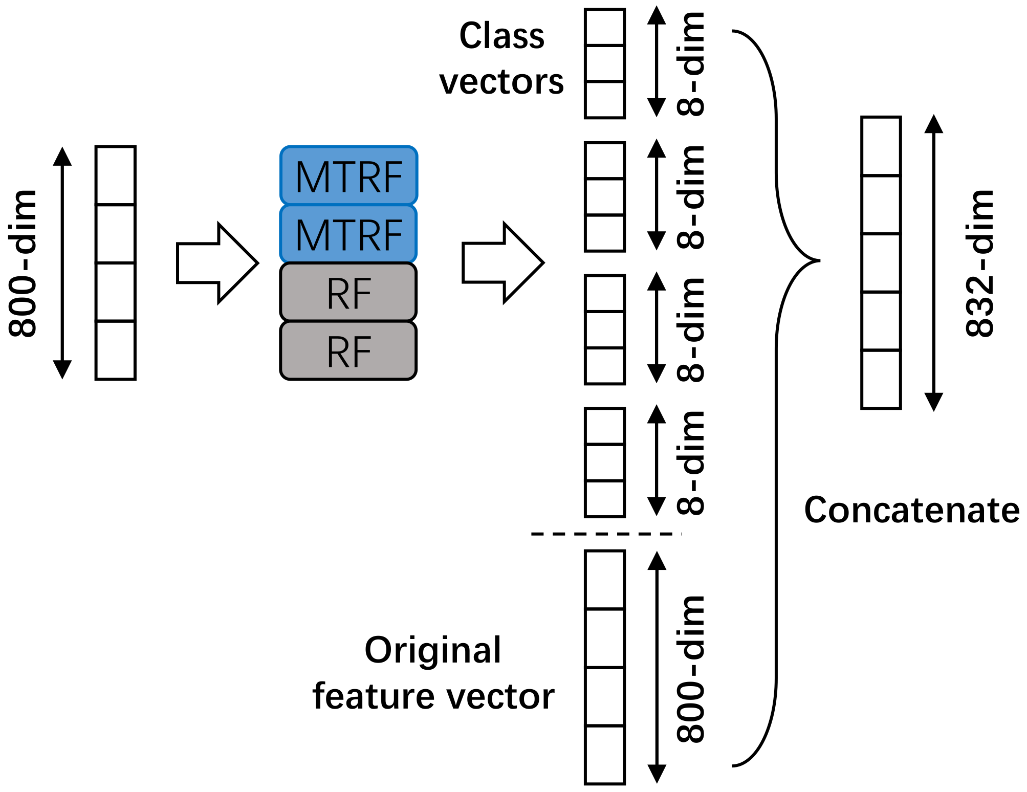
Concretely, we extract dense trajectories from an incomplete video and utilize bag-of-words model to build the original video feature vector, which is then input into the first level of the MTDF. At each level, one forest generates one class vector indicating the probability that this video belongs to each category. Then, as shown in Figure 2, four class vectors constructed by forests of a level are concatenated with the original feature vector as a new feature, which is input into the next level of the MTDF. Finally, the four generated class vectors of the last level are averaged into one class vector, and the action category corresponding to the largest element is treated as the predicted result.
In order to reduce the risk of over-fitting, k-fold cross validation is employed to build each forest. Particularly, we divide the training set into k groups and utilize groups for constructing a forest in each turn. An average of k class vectors is adopted as the ultimate class vector. Different from traditional random forest, a multi-task random forest is trained on incomplete videos annotated with both action category label and observation ratio label. As shown in Figure 1, during training, features annotated with both action category label and observation ratio label are sent to multi-task random forests in the first level, while the same features annotated with action category label are input into traditional random forests. In the following section, we will describe the construction of multi-task random forest in our framework in detail.
3.2. Random Forest
In our multi-task deep forest framework, two random forests [9] are utilized in each level of cascade. A random forest is an ensemble of decision trees and its principle is to let the trees vote for the most popular class. Suppose that a training set containing M samples is input into a random forest. Each sample includes a feature vector and an action category label . In the construction of a decision tree, randomness is introduced by randomly generating several splitting schemes for a node. When a group of samples arrives at a node, the information gain of each split scheme will be calculated by the action labels. Then, the scheme with the largest information gain is selected as a best scheme and is utilized for splitting the node into a left child node and a right child node. The node will continue to split until the samples that reach the node are of the same class or the node reaches its maximum depth. For a test sample input into a random forest, the sample will traverse from the root node of each tree until it reaches a leaf node. The proportion of samples of each action category in the leaf node will be defined as a class vector , and the class vector will be regarded as the output of the decision tree. The average of the class vectors generated by all decision trees in the random forest is the final output of the random forest.
3.3. Multi-Task Random Forest
A multi-task random forest is an ensemble classifier composed of multiple multi-task decision trees. Suppose that the training set contains M segmented videos with known observation ratios. Each sample in D contains a feature vector , an action category label , and an observation ratio label , where F is the number of features in a feature vector and K is the number of action categories. In order to reduce the association among different multi-task decision trees and enhance the overall performance of multi-task random forest, we employ the Bootstrap [20] method to generate a subset from the original training set D for each multi-task decision tree.
3.3.1. Construction of a Multi-task Decision Tree
In the construction of a multi-task decision tree, we keep a node sequence S and a pending node sequence Q. The element in the node sequence S is (,l,f,,,,,), where is the node ID, l represents the depth, f indicates the parent node, , are the left child node and the right child node, represents the split feature, is the split value, and is the action category vector. In particular, if the node is an intermediate node, is null, and, if the node is a leaf node, ,,, are null. The element in the pending node sequence Q is (,l,f,), where is the node ID, l represents the depth, f indicates its parent node, and is a dataset including all samples arriving at this node.
At first, a root node (1,1,0,) is crested and is put into Q, then a variable is initialized as 1. Then, we take the first node (,l,f,) in Q, and remove it from Q. If l is equal to the preset maximum depth of multi-task decision tree or samples in belong to the same categories on both action category label and observation ratio label, the node is regarded as a lead node; otherwise, the node is an intermediate node.
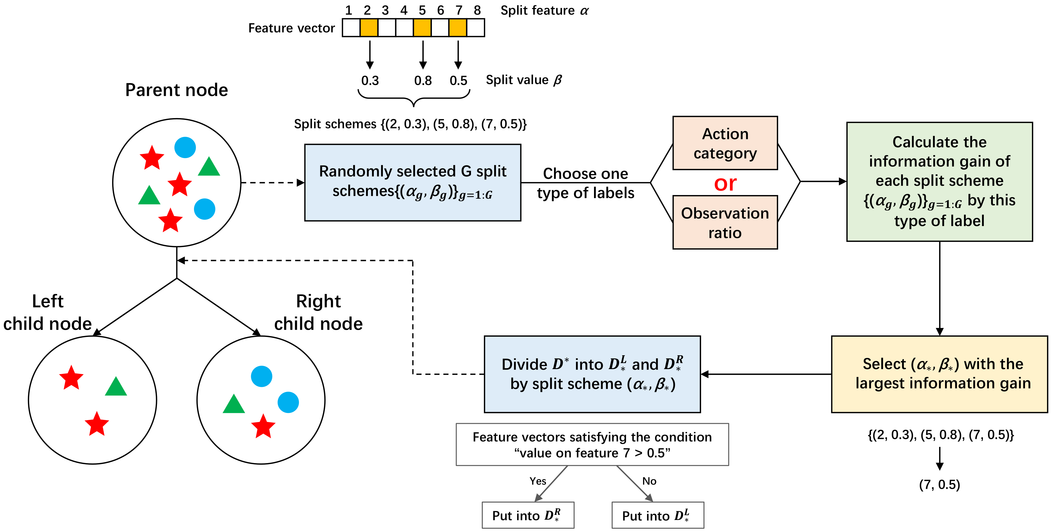
For an intermediate node (,l,f,) taken from sequence Q, procedures of node split are illustrated in Figure 3. A group of split schemes are generated, where is a randomly selected feature candidate and represents the split value generated according to values of samples in on feature . Each scheme divides the dataset into two subsets and . The former contains samples whose value on feature is smaller than , and the latter is composed of samples whose value on feature is bigger than . Then, the best scheme is chosen from for node split based on information gain maximization. Since each sample in has two labels, namely action category and observation ratio, we need to choose one type of label for calculating information gain.
Particularly, if the observation ratio labels of all the samples in are consistent, the information gain is calculated according to the action category label. Assuming that the proportion of samples in belonging to the k-th action is , the information entropy of can be defined as
where K is the number of action categories. For split scheme , the information entropy EntAction of and the information entropy EntAction of can be calculated in terms of Equation (1) as well. Accordingly, the information gain of utilizing split scheme is computed as
where indicates the number of samples in dataset D. Split scheme with the largest information gain is selected for node split according to Equation (3), and it divides the dataset into and .
Similarly, if all the samples in belong to the same action, the information gain is calculated according to the observation ratio label. Supposing that the proportion of the samples in with the j-th observation ratio label is , the information entropy is defined as
where the number of discrete observation ratios is 10. For split scheme , the information entropy EntRatio of and the information entropy EntRatio of can be calculated in terms of Equation (4). Next, the information gain split scheme is calculated as
The split scheme with the largest information gain is regarded as the best split scheme and is adopted for node split:
More frequently, samples in belong to different categories in terms of action label or observation ratio label. In this case, one type of label is randomly selected for calculation of information gain. Specifically, a predefined parameter [0,1] and a random variable are employed to control the selection. If , an action label is chosen to calculate the information gain GainAction for each scheme , and the best scheme is determined according to Equation (3). Otherwise, an observation ratio label is utilized to compute the information gain GainRatio, and Equation (6) is employed to choose the split scheme.
After dividing into and , the ID of the left child node is and the ID of the right child node is . Then, the current intermediate node is expressed as (,l,f,,,,,) and is further put into the node sequence S. Meanwhile, the left child node (,,,) and the right child node (,,,) are put into the pending node sequence Q. Then, the node counter is updated as .
For a leaf node (,l,f,) taken from sequence Q, we need to calculate the action category vector indicating the possibility that samples arriving at the leaf node belonging to each action category. To this end, we calculate the proportion of samples in belonging to the k-th action and create a class vector for this leaf node. Then, the leaf node is expressed as (,l,f,,,,,) and put it into the node sequence S.
Finally, if the pending node sequence Q is not empty, we will take the first node in Q again, or the construction of this multi-task decision tree is completed. The main steps of how to construct a multi-task decision tree are summarized in Algorithm 1.
3.3.2. Class Vector of a Multi-Task Random Forest
For a test sample input into a multi-task random forest, the sample will traverse from the root node of each tree until it reaches a leaf node. The class vector of the arrived leaf node is regarded as the output of the multi-task decision tree. An average of class vectors output from all the multi-task decision trees forms the final class vector of the multi-task random forest.
| Algorithm 1 Construction of a multi-task decision tree |
| Input: a training set // |
| Output: a node sequence S |
| 1: create a node sequence S storing settled nodes and a pending node sequence Q containing unsettled nodes; |
| 2: create the root node as (1,1,0,D’) and put it into Q; |
| 3: // the total number of generated nodes |
| 4: while Q is not do |
| 5: take out the first node (,l,f,) of Q; |
| 6: if l is equal to the preset maximum depth or samples in belong to the same categories on both action category label and observation ratio label then |
| 7: // the current node is a leaf node |
| 8: put the current node into S; |
| 9: else |
| 10: // the current node is an intermediate node need to be split |
| 11: randomly select G split schemes , and each scheme splits samples in into two subsets and ; |
| 12: generate a random value and compare it with a predefined parameter ; |
| 13: if or samples in belong to the same categories on observation ratio label then |
| 14: //evaluate each split scheme in terms of action labels of samples in |
| 15: for g is 1 to G do |
| 16: calculate the information gain GainAction according to Equation 2 |
| 17: end for |
| 18: choose the best split scheme according to Equation 3, and the dataset is divided into subsets and ; |
| 19: else |
| 20: //evaluate each split scheme in terms of observation ratio labels of samples in |
| 21: for g is 1 to G do |
| 22: calculate the information gain GainRatio according to Equation 5 |
| 23: end for |
| 24: choose the best split scheme according to Equation 6, and the dataset is divided into subsets and ; |
| 25: end if |
| 26: //put the current node into S |
| 27: //put the left child node into Q |
| 28: //put the right child node into Q |
| 29: end if |
| 30: |
| 31: end while |
| 32: return S |
4. Experiments
We evaluate our method on two datasets, and compare it with other methods. Section 4.1 shows the details of these two datasets and the experimental setup. The results of our MTDF and comparisons are shown in Section 4.2. Additionally, we analyze the influence of several key parameters in Section 4.3.
4.1. Datasets and Experimental Setup
The proposed MTDF approach is evaluated on two datasets: the UT-Interaction dataset including Set 1 (UT-I #1) and Set 2 (UT-I #2) [21], and the BIT-Interaction dataset [22]. UT-I #1 contains six types of human interactions, i.e., shaking hands, hugging, kicking, pointing, punching, and pushing, which were collected on a parking area from real surveillance videos. Each human interaction has 10 videos performed by 10 groups of participants. UT-I #2 shares the same classes of interactions with UT-I #1, but the background movements and camera jitters are larger over UT-I #1. On both UT-I #1 and UT-I #2 datasets, we utilize a 10-fold leave-one-out evaluation strategy.
The BIT-Interaction dataset consists of eight types of human interactions, each of which contains 50 videos. Complex background in this dataset poses great challenges for action prediction. In order to evaluate the proposed method, we take the first 34 videos in each class for training and utilize the last 16 videos in each class for testing.
The dense trajectory features [6] are extracted from videos in both UT dataset and BIT dataset, and the bag-of-words model is employed to encode these dense trajectory features, following the experiment settings in [1,4]. Crucially, in the following experiments, we set for all multi-task decision trees, which means there is equal probability of using action category label or observation ratio label to calculate the information gain for splitting.
4.2. Experimental Results
For more visible comparisons, we divide the experimental results into three parts. Comparison between MTDF and gcForest is shown in Section 4.2.1. Meanwhile, comparisons with other methods on UT-dataset and BIT-dataset are presented in Section 4.2.2 and Section 4.2.3, respectively. Due to the randomness of random forest and multi-task random forest, our method is run for 5 times and the average results are reported in this section.
4.2.1. Comparison between MTDF and gcForest
In order to evaluate the effectiveness of the proposed multi-task deep forest, we compare it with the original gcForest [8] on the UT-I #1, UT-I #2, and BIT datasets. The comparison experiments are summarized in Table 1.
On the UT-I #1 dataset, the proposed MTDF has achieved better or equal performance over the original gcForest at all observation ratios. Particularly, the MTDF achieves an improvement of 3.33% when the observation ratio is 0.4. On the UT-I #2 dataset, the proposed MTDF performs better than gcForest in most cases, and makes an improvement of about 4% at observation ratio 0.2. On the BIT dataset, our MTDF has achieved 0.15%-2.19% improvements over gcForest when more than 10% of videos are observed. In summary, it is effective to introduce an observation ratio label as an extra task during training, and our MTDF has shown improvement towards gcForest for action prediction. In particular, utilizing the observation ratio labels in the node splitting enhances the randomness of decision trees, which improves the discriminative power of MTDF.
4.2.2. Results on the UT-I #1 and UT-I #2 Datasets
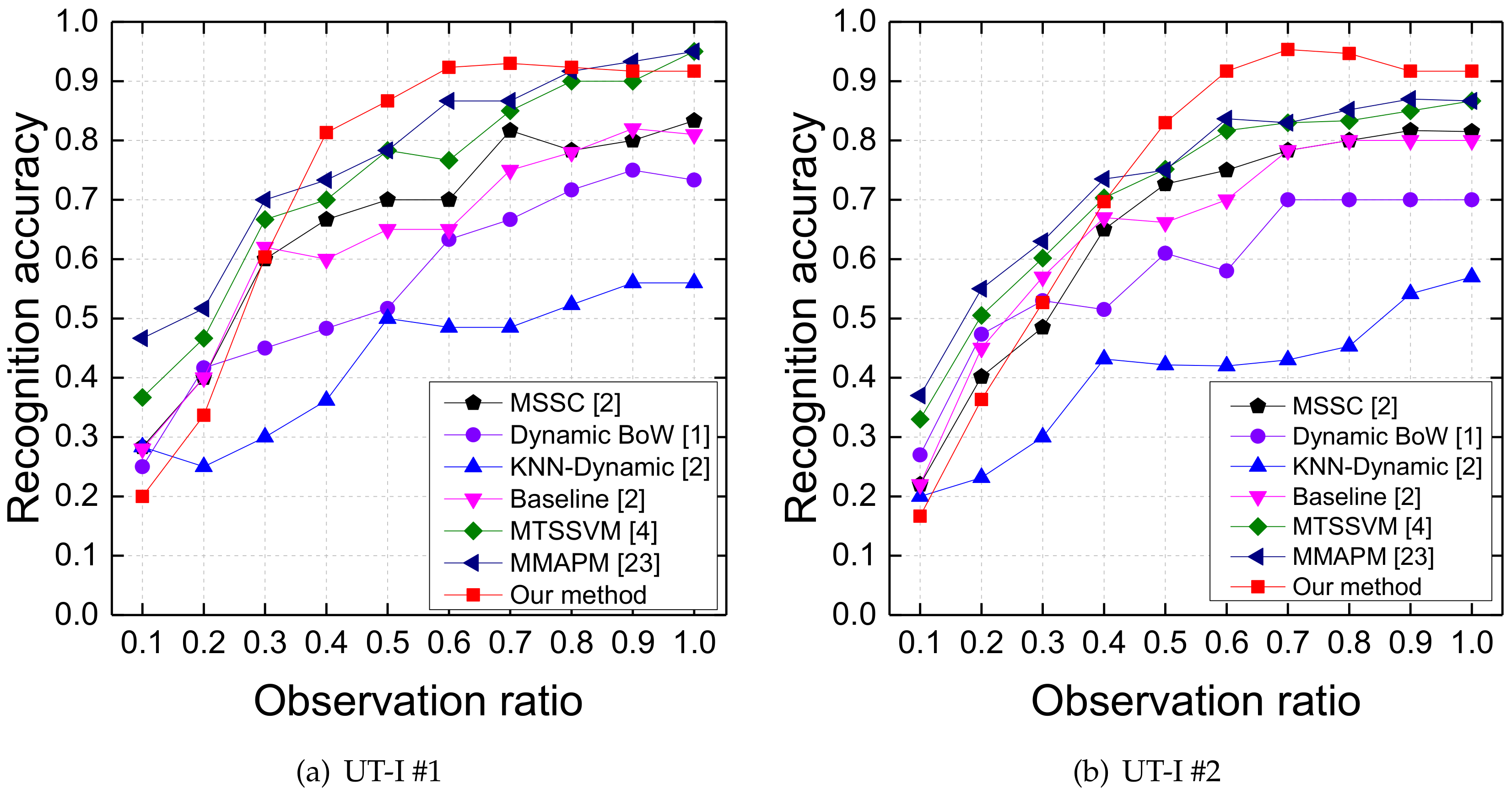
Our MTDF is compared with DBoW [1], MSSC [2], MTSSVM [4], and MMAPM [23] on the UT-I #1 and UT-I #2 datasets. In addition, KNN-Dynamic and the baseline method adopted in [2] are also employed in comparison. Our experiments utilize the same evaluation strategy as that in [2].
The comparison results on UT-I #1 dataset are shown in Figure 4a. Compared with the other methods, MTDF achieves better performance at {0.4, 0.5, 0.6, 0.7}. When only the first 40% frames of the testing videos are observed, recognition accuracy of our method is 81.33%. Then, the recognition accuracy of our method reaches 93% when the testing videos have been observed 70% frames. These results are much better than others at the same observation ratios. Our method does not perform well at observation ratio 0.1 because the video is so short that we cannot extract enough effective trajectories.
Figure 4b summarizes the comparison results on UT-I #2 dataset. When more than 40% frames of the testing videos are observed, MTDF is able to achieve higher recognition accuracy than all the compared methods. When only the first 50% frames of the testing videos are observed, our MTDF achieves 83% recognition accuracy, which is much higher than other comparison approaches at the same observation ratio and even higher than MSSC, DBoW, and KNN-Dynamic with full observations.
4.2.3. Results on the BIT Dataset
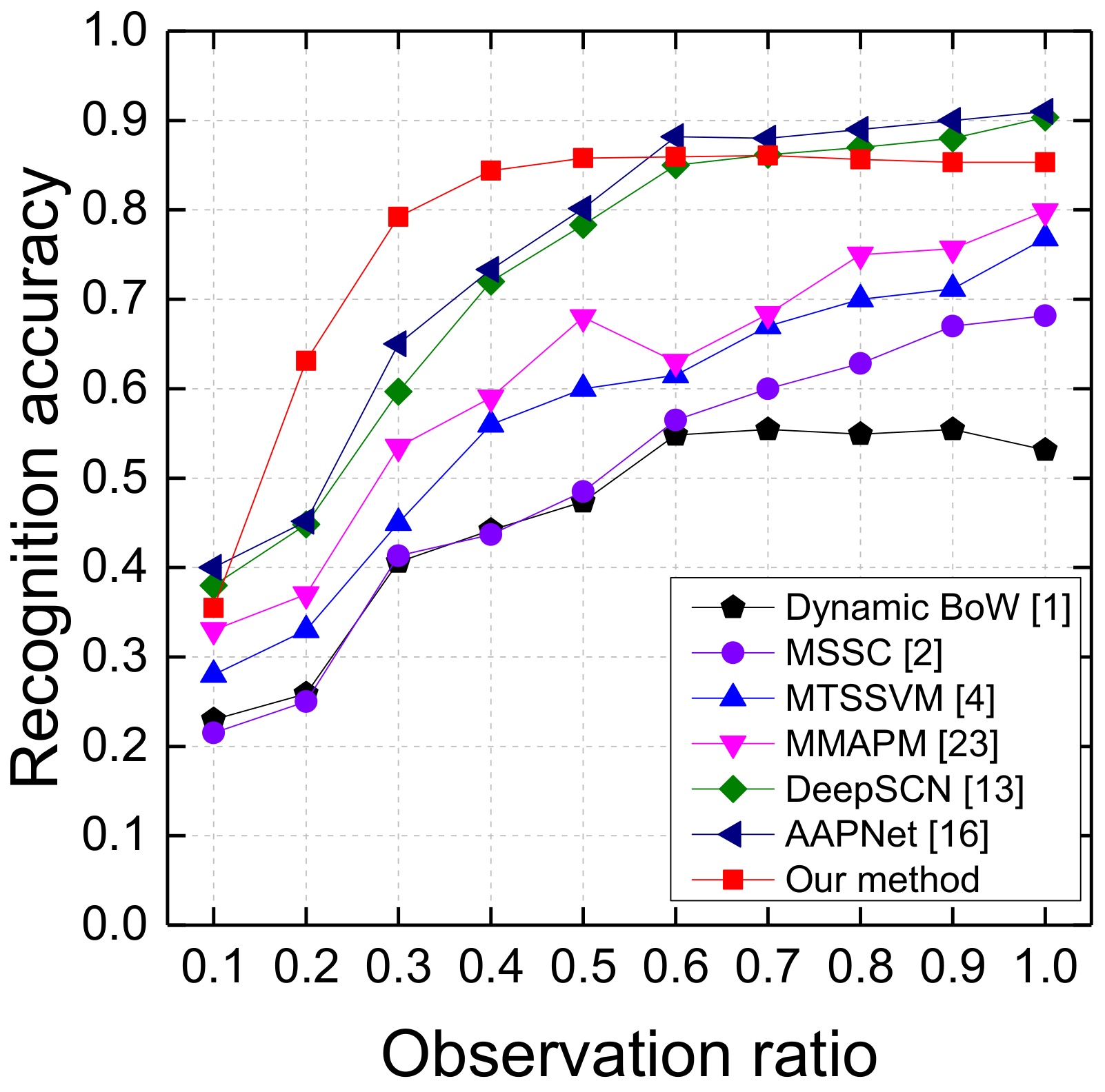
We also conduct experiments on the BIT-interaction dataset and compare the proposed MTDF with Dynamic BoW [1], MSSC [2], MTSSVM [4], MMAPM [23], DeepSCN [13], and AAPNet [16]. The comparison results on BIT dataset are shown in Figure 5.
Overall, the proposed MTDF outperforms MMAPM [23], MTSSVM [4], MSSC [2], and Dynamic BoW [1] at all observation ratios, and achieves comparable performance with DeepSCN [13] and AAPNet [16]. Different from UT-I #1 and UT-I #2, effective trajectory information can be extracted at the first 10% frames of the videos on the BIT-interaction dataset. Therefore, the proposed MTDF achieves 35.47% prediction accuracy at observation ratio 0.1. For observation ratios 0.2, 0.3,0.4, and 0.5, the prediction performance of MTDF is much better than the other comparison approaches. Particularly, MTDF achieves 63.13% prediction accuracy at observation ratio 0.2, which is 17.96% over AAPNet [16] and 18.3% over DeepSCN [13]. The prediction performance of MTDF does not increase significantly when the observation ratio is more than 0.6. One possible reason is that the key information for action prediction has been captured using the first 60% frames.
4.3. Effects of Parameters
In this section, we talk about several key parameters in the construction of MTDF. To this end, we conduct experiments on the UT-I #1 dataset and analyze the influence of parameters.
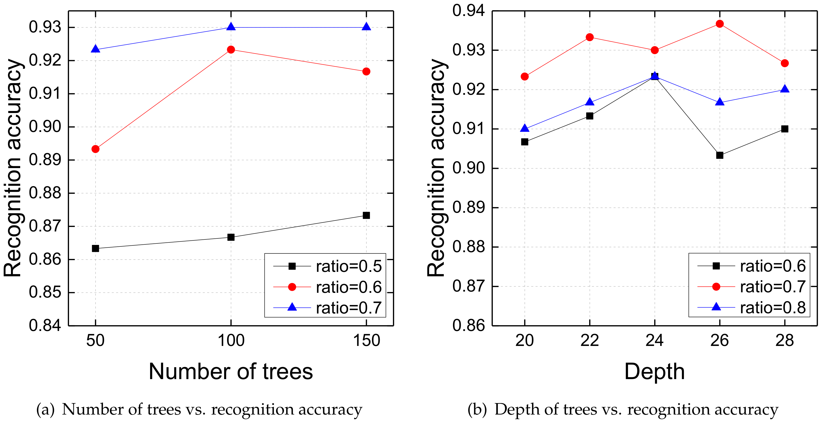
In considering the computational complexity of forest construction, we set the number of trees in a forest and limit the maximum depth of each decision tree. Figure 6a demonstrates the accuracy trend with different numbers of decision trees at observation ratios 0.6, 0.7, and 0.8. When the number of trees is less than 100, building more trees makes the accuracy improve continuously. Then, the recognition accuracy tends to be stable when there are more than 100 trees in each forest. In general, the prediction accuracy increases as the number of trees increases, and convergence is at a certain value. Figure 6b shows how the maximum depth of each decision tree affects the action prediction performance. Generally, with the increase of depth, the curves of different observation ratios rise first and then decline slightly and stabilize gradually. One reasonable explanation is that very deep decision trees may overfit the training data and reduce the action prediction performance on testing data.
5. Conclusions
In this paper, we have presented a novel Multi-Task Deep Forest framework for predicting actions from partially observed videos. In the construction of Multi-Task Deep Forest, we have utilized the observation ratio to evaluate the temporal progress of training incomplete videos and treated video temporal progress analysis as another task relevant to action prediction tasks. Experimental results on the UT-Interaction and the BIT-Interaction datasets show the superior performance of Multi-Task Deep Forest over the original single-task gcForest, which demonstrates that incorporating video observation labels during training can improve the action prediction performance. Moreover, the Multi-Task Deep Forest achieved better or comparable performance over the existing action prediction methods on both datasets, which has verified the effectiveness and reasonability of the Multi-Task Deep Forest.
Author Contributions
Investigation, T.Y.; Supervision, C.L., Z.Y., and X.S.; Writing—original draft, T.Y.; Writing—review and editing, C.L. and Z.Y. All authors have read and agreed to the published version of the manuscript.
Funding
This work was supported in part by the Foundation of Liaoning Educational Committee under Grant No. JYT19029, and in part by the Talent Scientific Start-up Project of Shenyang Aerospace University under Grant No. 18YB39, and in part by the National Natural Science Foundation of China (NSFC) under Grant No. 61602320.
Conflicts of Interest
The authors declare no conflict of interest.
Abbreviations
The following abbreviations are used in this manuscript:
| MTDF | Multi-Task Deep Forest |
| MTRF | Multi-Task Random Forests |
| RF | Random Forest |
References
- Ryoo, M.S. Human activity prediction: Early recognition of ongoing activities from streaming videos. In Proceedings of the IEEE International Conference on Computer Vision, Barcelona, Spain, 7 November 2011; pp. 1036–1043. [Google Scholar]
- Yu, C.; Barrett, D.; Barbu, A.; Narayanaswamy, S.; Song, W. Recognize Human Activities from Partially Observed Videos. In Proceedings of the IEEE Conference on Computer Vision & Pattern Recognition, Portland, OR, USA, 23–28 June 2013; pp. 2658–2665. [Google Scholar]
- Lan, T.; Chen, T.C.; Savarese, S. A Hierarchical Representation for Future Action Prediction. In Proceedings of the European Conference on Computer Vision, Zurich, Switzerland, 6–12 September 2014; pp. 689–704. [Google Scholar]
- Yu, K.; Kit, D.; Yun, F. A Discriminative Model with Multiple Temporal Scales for Action Prediction. In Proceedings of the European Conference on Computer Vision, Zurich, Switzerland, 6–12 September 2014; pp. 596–611. [Google Scholar]
- Laptev, I. On Space-Time Interest Points. Int. J. Comput. Vis. 2005, 64, 107–123. [Google Scholar] [CrossRef]
- Wang, H.; Schmid, C. Action Recognition with Improved Trajectories. In Proceedings of the IEEE International Conference on Computer Vision, Paris, France, 11 September 2014; pp. 3551–3558. [Google Scholar]
- Liu, C.; Wu, X.; Jia, Y. A hierarchical video description for complex activity understanding. Int. J. Comput. Vis. 2016, 118, 240–255. [Google Scholar] [CrossRef]
- Zhou, Z.H.; Feng, J. Deep Forest: Towards An Alternative to Deep Neural Networks. In Proceedings of the International Joint Conferences on Artificial Intelligence, Melbourne, Australia, 19–25 August 2017; pp. 3553–3559. [Google Scholar]
- Breiman, L. Random Forests. Mach. Learn. 2001, 45, 5–32. [Google Scholar] [CrossRef] [Green Version]
- Wang, H.; Yang, W.; Yuan, C.; Ling, H.; Hu, W. Human activity prediction using temporally-weighted generalized time warping. Neurocomputing 2017, 225, 139–147. [Google Scholar] [CrossRef]
- Feng, Z.; Torre, F.D.L. Generalized Time Warping for Multi-modal Alignment of Human Motion. In Proceedings of the IEEE Conference on Computer Vision & Pattern Recognition, Providence, RI, USA, 16–21 June 2012; pp. 3551–3558. [Google Scholar]
- Ma, S.; Sigal, L.; Sclaroff, S. Learning Activity Progression in LSTMs for Activity Detection and Early Detection. In Proceedings of the IEEE Conference on Computer Vision & Pattern Recognition, Las Vegas, NV, USA, 26 June 2016; pp. 1942–1950. [Google Scholar]
- Kong, Y.; Tao, Z.; Yun, F. Deep Sequential Context Networks for Action Prediction. In Proceedings of the IEEE Conference on Computer Vision & Pattern Recognition, Honolulu, HI, USA, 21–26 July 2017; pp. 1473–1481. [Google Scholar]
- Singh, G.; Saha, S.; Sapienza, M.; Torr, P.; Cuzzolin, F. Online Real-time Multiple Spatiotemporal Action Localisation and Prediction. In Proceedings of the IEEE International Conference on Computer Vision, Venice, Italy, 22–29 October 2017; pp. 3637–3646. [Google Scholar]
- Wang, D.; Yuan, Y.; Wang, Q. Early Action Prediction with Generative Adversarial Networks. IEEE Access 2019, 7, 35795–35804. [Google Scholar] [CrossRef]
- Kong, Y.; Tao, Z.; Fu, Y. Adversarial Action Prediction Networks. IEEE Trans. Pattern Anal. Mach. Intell. 2018. 1-1. Available online: https://0-ieeexplore-ieee-org.brum.beds.ac.uk/abstract/document/8543243 (accessed on 10 March 2020).
- Liu, J.; Shahroudy, A.; Gang, W.; Duan, L.Y.; Kot, A.C. SSNet: Scale Selection Network for Online 3D Action Prediction. In Proceedings of the IEEE Conference on Computer Vision and Pattern Recognition, Salt Lake City, UT, USA, 12–18 July 2018; pp. 8349–8358. [Google Scholar]
- Schydlo, P.; Rakovic, M.; Jamone, L.; Santos-Victor, J. Anticipation in Human-Robot Cooperation: A Recurrent Neural Network Approach for Multiple Action Sequences Prediction. In Proceedings of the IEEE International Conference on Robotics and Automation, Guangzhou, China, 17–19 November 2018; pp. 1–6. [Google Scholar]
- Liu, F.T.; Kai, M.T.; Yu, Y.; Zhou, Z.H. Spectrum of Variable-Random Trees. J. Artif. Intell. Res. 2008, 32, 355–384. [Google Scholar] [CrossRef] [Green Version]
- Efron, B.; Tibshirani, R.J. An Introduction to the Boot-Strap. Chapman & Hall 1993, 57, 1–436. [Google Scholar]
- Ryoo, M.S.; Aggarwal, J.K. UT-Interaction Dataset, ICPR contest on Semantic Description of Human Activities (SDHA). 2010. Available online: http://cvrc.ece.utexas.edu/SDHA2010/Human_Interaction.html (accessed on 10 March 2020).
- Kong, Y.; Jia, Y.; Fu, Y. Learning human interaction by interactive phrases. In Proceedings of the European Conference on Computer Vision, Florence, Italy, 7–13 October 2012. [Google Scholar]
- Kong, Y.; Fu, Y. Max-Margin Action Prediction Machine. IEEE Trans. Pattern Anal. Mach. Intell. 2015, 38, 1844–1858. [Google Scholar] [CrossRef]
Figure 1.
Overview of the proposed multi-task deep forest.

Figure 2.
Details of how to concatenate feature vectors at the first level. In this figure, we suppose that there are eight action categories.
Figure 2.
Details of how to concatenate feature vectors at the first level. In this figure, we suppose that there are eight action categories.

Figure 3.
Details of node split for an intermediate node in a multi-task decision tree.

Figure 4.
Prediction results on the UT-Interaction dataset.

Figure 5.
Prediction results on the BIT dataset.

Figure 6.
Recognition accuracy changes as the parameters are adjusted at different observation ratios r on UT-I #1.
Figure 6.
Recognition accuracy changes as the parameters are adjusted at different observation ratios r on UT-I #1.


Table 1.
Prediction results on UT-I #1, UT-I #2, and BIT dataset, using gcForest [8] and our multi-task deep forest
Table 1.
Prediction results on UT-I #1, UT-I #2, and BIT dataset, using gcForest [8] and our multi-task deep forest
| Observation ratio | 0.1 | 0.2 | 0.3 | 0.4 | 0.5 | 0.6 | 0.7 | 0.8 | 0.9 | 1.0 | |
| UT-I #1 | gcForest | 19.33% | 33.67% | 60.00% | 78.00% | 86.33% | 91.67% | 92.00% | 91.67% | 91.00% | 90.67% |
| MTDF | 20.00% | 33.67% | 60.33% | 81.33% | 86.67% | 92.33% | 93.00% | 92.33% | 91.67% | 91.67% | |
| UT-I #2 | gcForest | 16.67% | 32.33% | 51.33% | 68.00% | 83.33% | 90.67% | 93.67% | 93.33% | 92.00% | 92.00% |
| MTDF | 16.67% | 36.33% | 52.67% | 69.67% | 83.00% | 91.67% | 95.33% | 94.67% | 91.67% | 91.67% | |
| BIT | gcForest | 36.72% | 60.94% | 77.50% | 83.44% | 85.63% | 85.00% | 84.69% | 84.38% | 84.06% | 84.06% |
| MTDF | 35.47% | 63.13% | 79.22% | 84.38% | 85.78% | 85.94% | 86.09% | 85.63% | 85.31% | 85.31% | |
© 2020 by the authors. Licensee MDPI, Basel, Switzerland. This article is an open access article distributed under the terms and conditions of the Creative Commons Attribution (CC BY) license (http://creativecommons.org/licenses/by/4.0/).
Share and Cite
MDPI and ACS Style
Yu, T.; Liu, C.; Yan, Z.; Shi, X. A Multi-Task Framework for Action Prediction. Information 2020, 11, 158. https://0-doi-org.brum.beds.ac.uk/10.3390/info11030158
AMA Style
Yu T, Liu C, Yan Z, Shi X. A Multi-Task Framework for Action Prediction. Information. 2020; 11(3):158. https://0-doi-org.brum.beds.ac.uk/10.3390/info11030158
Chicago/Turabian StyleYu, Tianyu, Cuiwei Liu, Zhuo Yan, and Xiangbin Shi. 2020. "A Multi-Task Framework for Action Prediction" Information 11, no. 3: 158. https://0-doi-org.brum.beds.ac.uk/10.3390/info11030158
Note that from the first issue of 2016, this journal uses article numbers instead of page numbers. See further details here.