Forecasting Appliances Failures: A Machine-Learning Approach to Predictive Maintenance

Abstract

Heating appliances consume approximately $48\%$ of the energy spent on household appliances every year. Furthermore, a malfunctioning device can increase the cost even further. Thus, there is a need to create methods that can identify the equipment’s malfunctions and eventual failures before they occur. This is only possible with a combination of data acquisition, analysis and prediction/forecast. This paper presents an infrastructure that supports the previously mentioned capabilities and was deployed for failure detection in boilers, making possible to forecast faults and errors. We also present our initial predictive maintenance models based on the collected data.

1. Introduction

The industrial world is being transformed into a technological and data-centric world, named Industry 4.0 [1]. Companies are investing in data analytics to improve efficiency, productivity, and reduce costs. One of the main advantages is failure prediction and root-cause analysis [2], making possible to reduce the resources (and time) dedicated to reactive repairs while reducing failure events on critical equipment. An equipment failure, and subsequent reparation, can occur into a high expense to the company. As such, there is a strong need for Predictive Maintenance (PdM) solutions [3], especially addressing the prevention of component failure, with impact in production quality and client satisfaction (among many other factors). Therefore, predictive maintenance refers to the ability to forecast failures, ensuring that important operations are not disrupted as actions can be taken to prevent them. This is common practice for critical scenarios (military, aviation, power plants), and has been introduced to a wider range of products.

Despite the existence of several approaches to deal and implement PdM systems, such solutions generally fail at combining the acquisition, processing and predictive parts as a single platform. Therefore, in this work, we propose an efficient Big Data Service that can be instantiated for several PdM scenarios and environments. In particular, the presented system emerges from the “Smart Green Homes” (http://www.ua.pt/smartgreenhomes/) project, whose main goal is to develop a platform capable of dealing with the massive amount of data produced by the Industry 4.0 and provide a unified framework to acquire, store and analyse the data and extract relevant knowledge.

Our final application target consists of identifying and predicting failures on a Heating, Ventilation, and Air-Conditioning (HVAC) system, specifically in boilers and heat pumps. For this purpose, we acquired and analysed real data from thousands of devices, operating at customer premises, over a wide range of product lines and scenarios. This work evolves from previous contributions [4], in which the identification of outliers through batch-processing and classification algorithms failed at providing enough information to tackle this problem. We note that since our main goal was to predict failures in real time, there was a need to develop a computational infrastructure allowing automatic data processing.

Based on this, the main contributions of this work are the following. First, we developed a framework capable of acquiring, storing and processing the necessary data from several heating appliances, which contains device operational data. Moreover, we developed methods to analyse and predict equipment failure based on the previously mentioned data. It is important to notice that we are considering real data and, consequently, it is more frequent to find normal operation than failure states. As such, we have to deal with an unbalanced dataset as the frequency of outliers is lower than the normal states (standard operation), creating a bias in the classification algorithms which have a preference on the most common classes. The collected dataset is also quite complex, we acquired several alphanumeric features from multiple devices running different firmware versions. Therefore, an important part of the presented work must deal with data normalisation and the development of techniques that can be applied to multivariate time-series data.

This paper is organised as follows. Section 2 presents the state of the art of current solutions relevant to this work. In Section 3 we describe our solution for data acquisition and storage. In Section 4 we study the application of machine learning models to predict failures on the HVAC data. The results of our models are described in Section 5. Finally, we conclude in Section 6.

2. Related Work

The implementation of PdM solutions needs to take into account key aspects, such as the underlying scenario, the performance key indicators, and the metrics that should be defined to measure them [5]. Besides those, some other aspects are important to build an efficient PdM system, such as forecasting the key indicators, enabling institutions to make decisions according to the upcoming problems [6].

The PdM system requires the identification of the input variables, a target application, and the model that creates a relationship between them. After the development of the model, it is possible to obtain results that will be analysed and validated to make decisions that can help with the evaluation and optimisation of the overall system. This evaluation is very important for the analysis of the system reliability since companies build PdM solutions to reduce costs, and thus, the system should be economical and low risk.

It is important to evaluate the amount and quality of the available data. The existence of large amounts of data may require the application of reducing and normalisation methods. Another common issue is the lack of information about the target application, which will affect the relationship between the application and the inputs.

To mitigate these common issues, it is necessary to build a practical and comprehensible system that offers technologies with large storage capacity and speed of interaction [7].

An effective PdM solution is composed of the following key blocks (as depicted in Figure 1). The Data Source (such as sensors, where data is created) is the input block. Data Acquisition is responsible for the connection between data sources and the remaining architecture. Moreover, it is useful to keep the acquired data, as such a Data Storage block is used to store all the data. To bridge the Data Storage block with upper blocks, a Data Processing block is used [8]. Furthermore, a Data Mining block is implemented (as one of the upper blocks) to $\left(i\right)$ identify key features on data and $\left(ii\right)$ learn the relation between those features (input variables) and the target application. Finally, the other upper block, which interacts with the application user, is the Data visualisation block that shows important information about the application and the obtained predictions [9].

After the validation of the PdM solution, it is possible to integrate it with Quality Control systems. The PdM results are then used to control the applications and provide an extra maintenance indicator to the Quality Control systems [10]. This interaction can be helpful for the construction of systems that require notifications for detected faults and interaction with the application users such as the one presented in this paper.

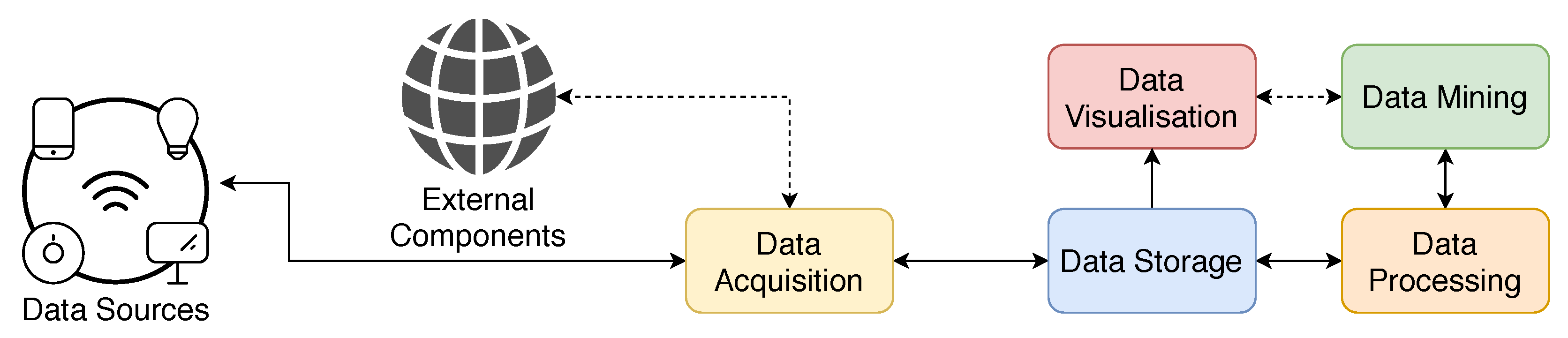
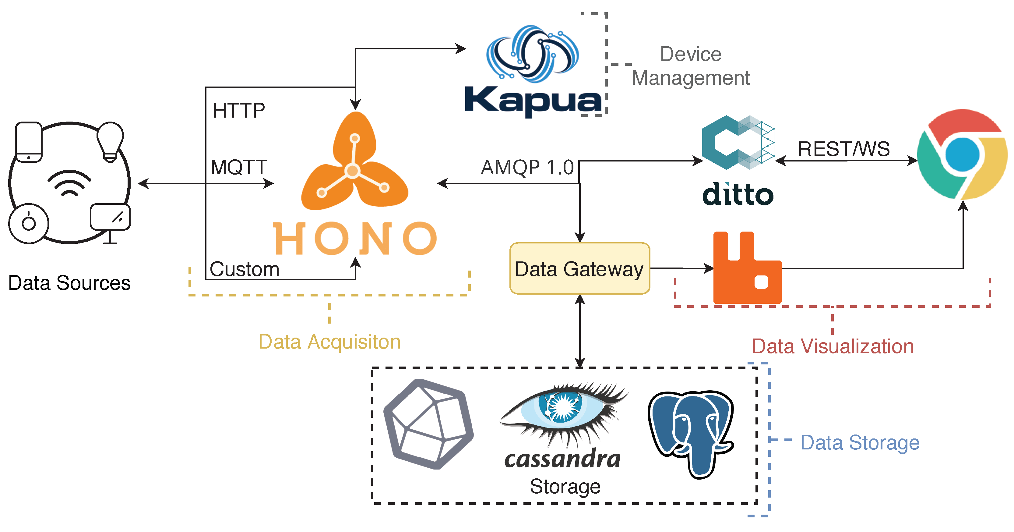
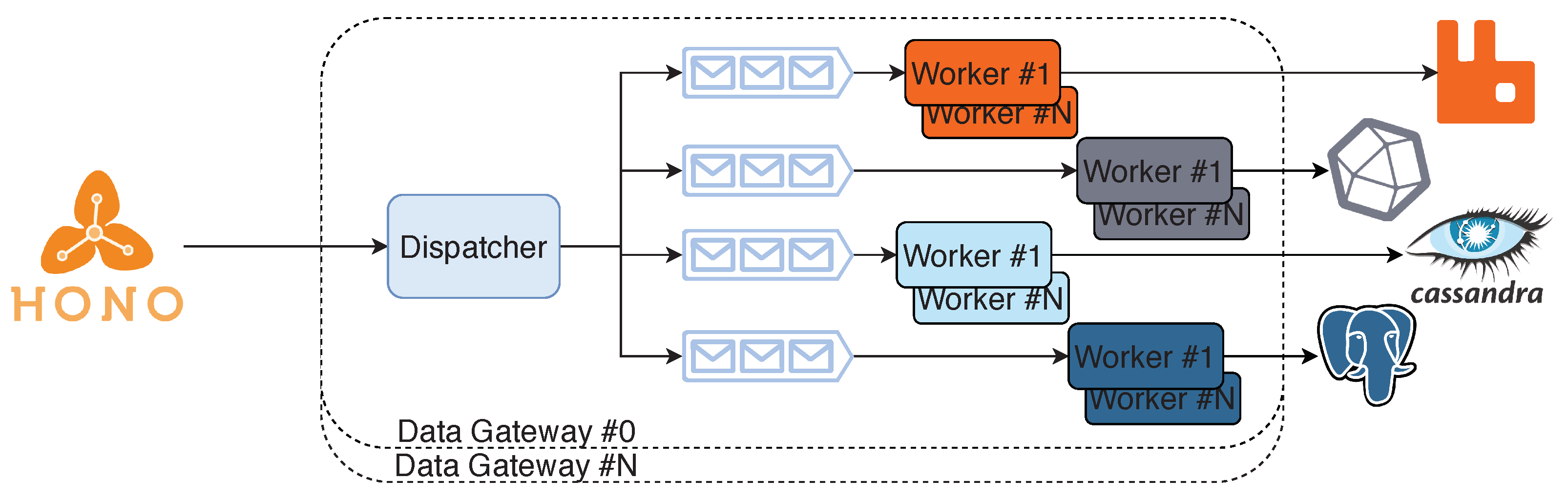
3. SCoT—Smart Cloud of Things

SCoT (Smart Cloud of Things) is an evolution from a previous solution, APOLLO [11], which aims to develop a generic platform for integration of Internet of Things (IoT) scenarios, with integration in Telecom networks. Therefore, it considers aspects related to network, device management, services, and applications.

The SCoT platform should enhance resource optimisation and provide a flexible platform for massive and dynamic IoT scenarios. One way to improve resource optimisation is through a careful division of the platform into micro-services that can be deployed into containers. The proposed solution has the following advantages:

• Distributed architecture—Implementing a multi-node distributed platform which allows distributing workloads evenly among other available machines and making it fault-tolerant by keeping track of the cluster’s health.
• Service replication with load balancing—The implementation allows creating copies of the same service and distributing traffic through these copies aiming to maximise the performance;
• Easier to scale infrastructure and applications—This type of implementation facilitates the way scaling operations of either the cluster or the services of an application are handled, allowing a near-zero downtime when updating services or when scaling the actual cluster;
• Automatic deployment of the platform infrastructure with the application—Create a mechanism that allows deploying the platform with the application facilitating future testing or developing scenarios.

The platform architecture is depicted in Figure 2, and it is based on 3 key services: Hono, Ditto and Kapua. Eclipse Hono (https://www.eclipse.org/hono/) is an Internet of Things (IoT) suite that enables connecting a large number of IoT devices using a major set of services capable of handling different protocols used in the IoT world such as MQTT, AMQP, HTTP or CoAP. Hono collects telemetry data from these devices and discloses it through an API, this suite is based on containers and provides support for a wide range of container orchestration environments.

Eclipse Ditto (https://www.eclipse.org/ditto/) implements a software pattern called “digital twins”. A digital twin is a virtual, cloud-based, representation of his real-world counterpart (real-world “Things”, e.g., sensors and actuators). The technology mirrors potentially millions and billions of digital twins residing in the digital world with physical “Things”. This simplifies developing IoT solutions for software developers as they do not need to know how or where exactly the physical “Things” are connected. With Ditto, a “thing” can just be used as any other web service via its digital twin. As with Hono, Ditto is based on containers and provides support for a wide range of container orchestration environments.

Eclipse Kapua (https://www.eclipse.org/kapua/) is a modular integration platform for IoT devices and smart sensors that aims at bridging Operation Technology with Information Technology. Eclipse Kapua focuses on providing comprehensive management of edge IoT nodes including their connectivity, configuration, and application life cycle. In short, this component is responsible for the device management, registration and authentication.

In addition to the previously detailed services, other services need to be included to enrich the platform. These include a Data Gateway that connects to several databases and a broker.

As stated in [12] due to the inherent complexity of IoT scenarios it is quite difficult to have a single database model to store all the information and still provide meaningful structure for Data Processing components. For that reason, instead of sticking with a single database model, we developed a Data gateway that transforms the data and stores it accordingly in the instantiated databases. In our implementation, we used 3 different databases: Apache Cassandra, PostgreSQL and InfluxDB. Each one of them is a mature representation of NoSQL, Relational and Time-Series databases, respectively. Depending on the specific scenarios, data can be consumed from any of the available databases. Furthermore, we also instantiated a RabbitMQ broker to provide real-time access to the data stream.

The Data Gateway is one of the most important services in the redesigned architecture. It bridges the Hono communication framework with the Data Storage and a real-time broker. We designed this service to be capable of scaling vertically and horizontally, as depicted in Figure 3. The Gateway has a queue for each database backend, where multiple workers consume messages and store them into the respective database (horizontal scaling). Furthermore, there can be more than one gateway instantiated, as well as more than one worker per database per gateway, achieving vertical scalability.

The schema of the Relational and NoSQL databases was based on previous work [13]. The InfluxDB has a unique internal structure, to develop a generic store method we had to develop a recursive flat parser. The parser can flatten any JSON document. The flattened JSON is then parsed into individual components and inserted into the InfluxDB as individual streams.

4. Predictive Maintenance Models

In the previous section we described the platform that we developed to acquire the data from heating appliances. Given the data collected by the proposed application, we are now interested in developing a predictive model using machine learning to apply to it. The details of our experiments are provided below.

4.1. Problem Setting

Formally, given the heating appliances logs obtained so far, our aim is to predict a boiler malfunction and possible failure, within up to 7 days before it occurs. This is a relevant problem as it allows the industrial companies to take preventive measures to ensure the correct function of the appliance. A corrective measure can be a remote configuration of the appliance to send an expert to repair the boiler before it enters a critical state and stops working.

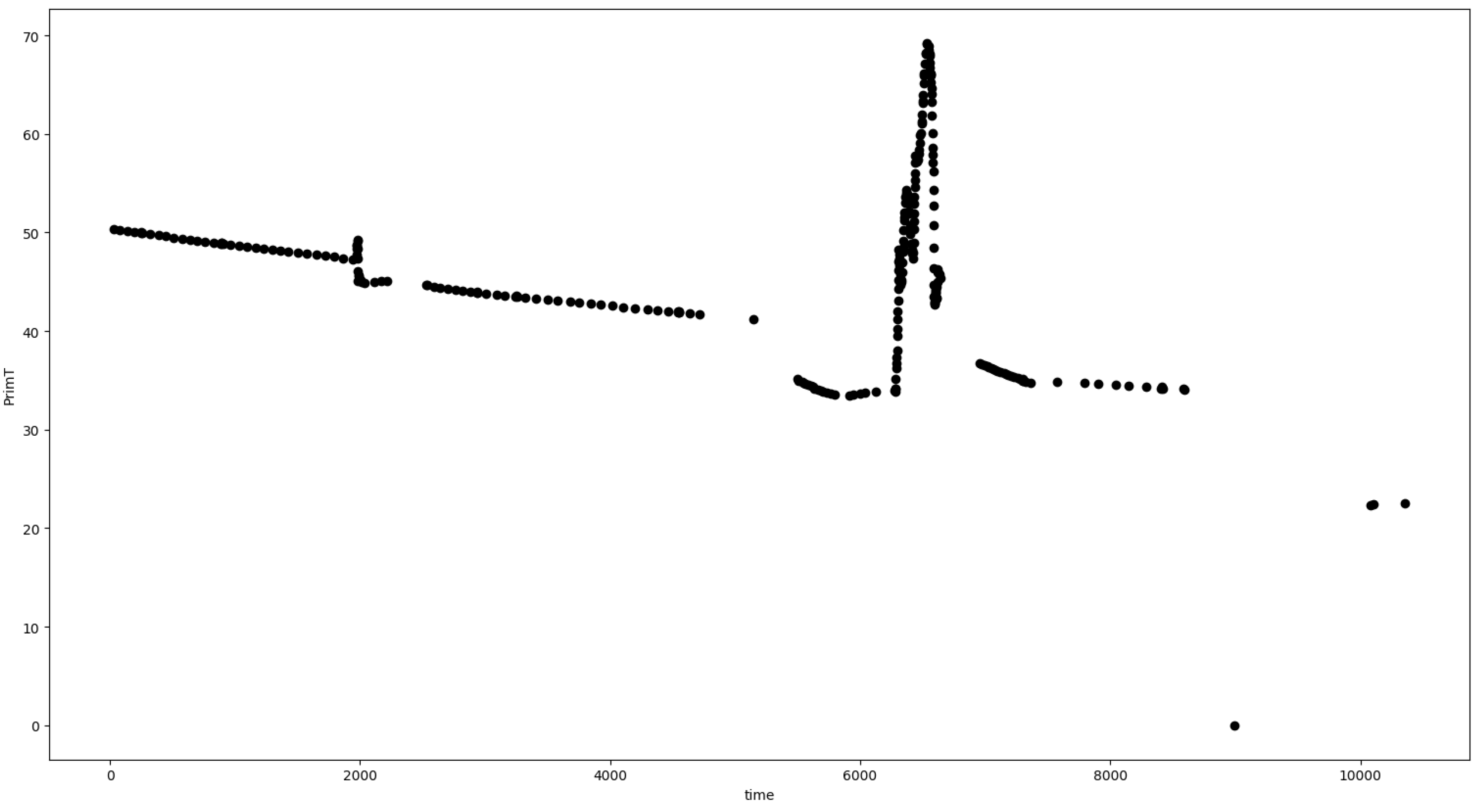
4.2. Data

As previously exposed, our dataset contains boilers operation values. These boilers, whose main function is to supply hot water to the customers, are installed in their houses. The data was collected for 16 months including information from 1000 appliances of ten different models. Nonetheless, given that some of the appliances only had information about one-month minimum, we considered a subset of around three consecutive complete months of data in this study.

Each boiler has sensors collecting data such as temperature, number of boiler starts, number of heating requests and duration of each cycle. In particular, the boiler state at a given timestamp is characterized by 91 features, including the level of malfunction at the current timestamp (which may be either none, light or severe). Two consecutive timestamps are spaced by at least a millisecond. Moreover, the appliances are programmed to send the values of a given feature if it changes, which leads to the existence of gaps in the data logs, as illustrated in

Table 1. Illustration of a log with missing data.

Time	PrimT	ChNoStart	BurnNoStart
07:42:44.304			1558.0
07:42:44.404	23.7	155.0
07:42:44.504		156.0
07:42:44.604	23.8		1559.0
07:42:44.704		155.0	1561.0

: at time 07:42:44.404 the values of PrimT and ChNoSart are updated but no value is registered for the variable BurnNoStart; in such case, for the latter feature, the value at time 07:42:44.404 is assumed to be the last value registered (1558.0). An example of the PrimT log with missing values is shown in Figure 4.

It is worth mentioning that among the data subset considered, around $90.8\%$ of the logs are associated with boilers working correctly (with no malfunction), while $8.8\%$ are associated with light faults and only $0.4\%$ are associated with severe faults, which are the most relevant type of faults as they require technical assistance to be solved.

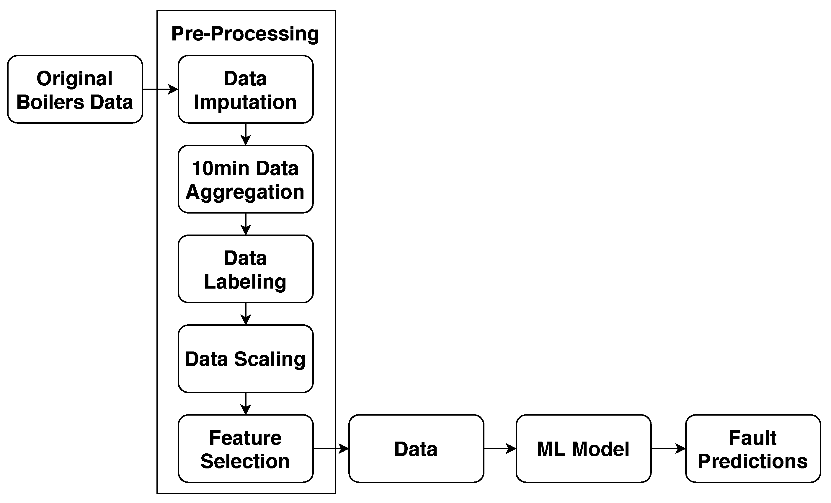
Data Pre-processing

Before defining our model, we had to pre-process the data by taking into account that:

• values were missing in the logs;
• in most of the cases, there was a log for each boiler at each millisecond, leading to a huge amount of data, which does not necessarily provide meaningful information;
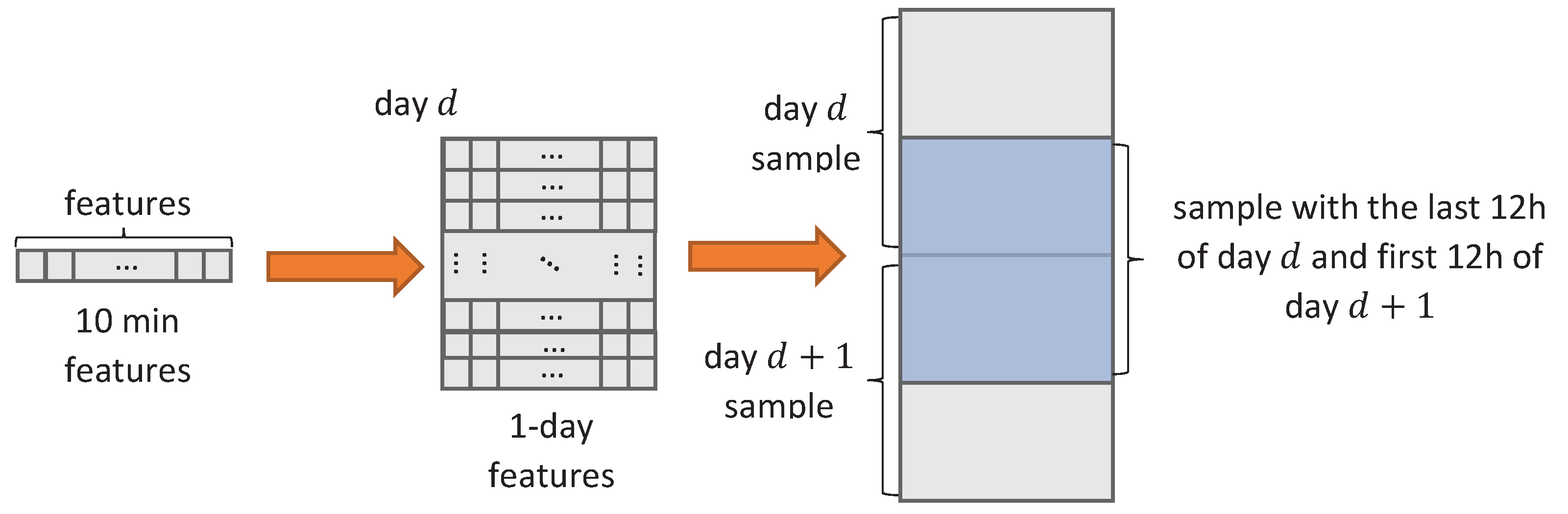
• the data must be re-shaped into supervised problem data format, i.e., for each log, we should set a fault class according to our problem setting;
• different features may assume a different scale of values;
• the number of features in the data was extremely large, which may compromise the learning speed and quality of the model.

Based on this, we started by applying an imputation procedure to fill the missing values. In our scenario, a missing value was set to the last value registered in such feature.

Given the filled version of the dataset, we aggregated the logs of each boiler by consecutive and non-overlapping periods of 10 min. We chose this time granularity to reduce the amount of data to process without compromising the quality of the data. We note that by considering 10 min intervals, we expect not to lose too much variability in the data.

Since we are dealing with supervised learning, we had to re-organise the data into observations and corresponding target classes. In our case, the target of a given observation is the worst level of malfunction observed in the following 7 days. In particular, there are three possible levels of malfunction: $\left(i\right)$ no fault (which means that the boiler is working correctly), $\left(ii\right)$ light fault (which means that the boiler is not working correctly but the problem can be solved by resorting to the appliance documentation) and $\left(iii\right)$ severe fault (which means that the boiler stopped working and technical assistance is required). Thus, if a severe fault occurred between days $t+1$ and $t+7$, then the target of such observation was set to the severe fault class. Otherwise, if a light fault occurred between days $t+1$ and $t+7$, then the corresponding target was set to the light fault class. The target of the observation was only set to no fault class if no faults were observed in the following week. Moreover, the data was split in the conventional $70\%$ of samples for training, $10\%$ for validation and $20\%$ for testing, and each feature was scaled to have zero mean and unit variance.

Finally, given the large number of features in the data, it is expected that some of them are not useful/meaningful to our task and consequently should not be considered. Therefore, we applied feature selection strategies to find the most relevant features. In particular, we applied a random forest classifier to our data to find the set of features that are most influential on the malfunction/fault types [14]. According to this method, around $75\%$ of the features are not relevant to our classification problem and therefore we discarded them from our dataset.

This process is summarised in Figure 5.

4.3. Models

Since the logs of a boiler may be regarded as a multivariate time-series and the current state of a given boiler is expected to be related with the following states, then considering each 10 min states separately (that is, without accounting for their temporal sequential component) may lead to loss of information.

To tackle this issue, we considered a time-aware learning model for our problem. In particular, we considered a Long Short-term Memory (LSTM) [15], a recurrent neural network architecture, designed to deal with sequential data. In our setting, we feed a sequence of 1-day boiler logs to the LSTM to predict if the corresponding boiler will fail in the next 7 days.

In particular, for each boiler, first we aggregated (sequentially) the logs by day so that we obtained matrices whose row i is the log of the boiler at the $i\mathrm{th}$ 10 min interval of the given day (this process is illustrated in Figure 6 (left)). Such data was used as input for the $LST{M}_0$ model. Additionally, to assess the impact of the temporal information in the model, we considered multiple distinct “augmented” training sets. In particular, for a given boiler, besides a training observation for day d and another for day $d+1$, we considered more training observations per pair of consecutive days in the dataset. These observations were generated by considering samples with information from two consecutive days. Thus, in $LST{M}_1$, for each boiler, we added a training sample containing the last 12 h of day d and the first 12 h of the following day, $d+1$ (this process is illustrated in Figure 6 (right)). The training datasets generated for $LST{M}_2,LST{M}_3,LST{M}_4$ models were generated similarly, with the difference that instead of considering only a training sample overlapping each pair of consecutive days, we considered 2,3 and 4 distinct samples, respectively. Based on this, we can think of $LST{M}_0$ as a model operating in a sliding window with no overlap, while $LST{M}_i$ (with $i\in \{1,2,3,4\}$) operates in a sliding window with overlap. In both settings, a window length of 144 observations of 10 min (1 day) is considered.

As a term of comparison, we also considered less complex and time-agnostic classifiers, namely a random stratified classifier, a random tree classifier and neural networks. For these models, the input was set to a single 10 min observation. Moreover, since neural networks are strongly affected by the class imbalance [16], we considered two settings: the traditional neuronal network (NN) and a sample weighted neuronal network (weighted NN) in which the error of each sample is weighted according to the frequency of their class in the dataset—the least the frequency of the target class, the largest the weight assigned to the corresponding observation.

Regarding the architecture of the network-based models, we considered varying architectures of 1, 2 or 3 hidden layers and 15, 25, 50 neurons. We note that more complex models were studied but no gain was observed and consequently, for simplicity, we did not consider them in this work.

4.4. Evaluation Metrics

Since we are dealing with an imbalanced dataset, we analysed the predictions quality for each of the tree classes. In particular, we computed the precision and recall for each of the classes. The precision of the model in class i is computed as:

$$precisio{n}_i=\frac{T{P}_i}{T{P}_i+F{P}_i},$$

(1)

and the corresponding recall is computed as:

$$recal{l}_i=\frac{T{P}_i}{T{P}_i+F{N}_i},$$

(2)

where $T{P}_i$ is the number of test observations correctly classified as class i, $F{P}_i$ is the number of test observations incorrectly assigned to the class i and $F{N}_i$ is number of test observations of the class i, incorrectly assigned by the model to another class. In our scenario the classes are $\{nofault, lightfault, severefault\}$.

To have a unified perspective of the precision and recall values, we also considered the f1-score, which is computed for each class $i\in \{nofault, lightfault, severefault\}$ as:

$$f{1}_i=2\frac{precisio{n}_i\times recal{l}_i}{precisio{n}_i+recal{l}_i}$$

(3)

Finally, we also considered 3 global metrics: accuracy, macro f1-score and Mathews Correlation Coefficient (MCC) [17]. We computed the global accuracy as:

$$accuracy=\frac{T{P}_{nofault}+T{P}_{lightfault}+T{P}_{severefault}}{N},$$

(4)

where N is the total number of samples in the test set. The macro f1-score is given by:

$$macro\_f1=\frac{f{1}_{nofault}+f{1}_{lightfault}+f{1}_{severefault}}{3},$$

(5)

MCC is computed by resorting to the confusion matrix (CM), in which $CM(i,j)$ is the number of test samples of class i assigned to class j. In more detail, given a problem of K classes, MCC is computed as:

$$MCC=\frac{{\sum }_{i,j,k=1}^K\left[CM(i,i)CM(k,j)-CM(j,i)CM(i,k)\right]}{\sqrt{\left({\sum }_{i=1}^K\left[\left({\sum }_{j=1}^{K}CM(j,i)\right)\times \left({\sum }_{k,l=1,k\ne i}^{K}CM(l,k)\right)\right]\right)\times \left({\sum }_{i=1}^K\left[\left({\sum }_{j=1}^{K}CM(i,j)\right)\times \left({\sum }_{k,l=1,k\ne i}^{K}CM(k,l)\right)\right]\right)}}$$

(6)

It should be noted that all but MCC metrics range from 0 to 1. In MCC the value can range from $-1$ to 1. In all the metrics considered, the higher the value, the better the predictor.

5. Results

A complete list of results is provided in

Table A1. Complete results from the fault prediction model. The following abbreviations were used. Hlayer, p, r, f1 and Acc stand for hidden layers, precision, recall, f1-score and accuracy, respectively.

Model	Architecture		No Fault			Light Fault			Severe Fault
	Hlayers	Neurons	P	R	F1	P	R	F1	P	R	F1	Acc	Macro F1	MCC
Dummy (stratified)	/	/	0.91	0.81	0.86	0.09	0.18	0.12	0	0.01	0.01	0.75	0.33	0
Decision Tree	/	/	0.9	0.85	0.87	0.03	0.06	0.04	0	0	0	0.77	0.3	−0.08
NN	1	15	0.92	0.86	0.89	0.12	0.16	0.14	0	0.01	0	0.79	0.34	0.05
		25	0.91	0.79	0.85	0.1	0.22	0.13	0.01	0.02	0.01	0.74	0.33	0.02
		50	0.91	0.82	0.86	0.09	0.16	0.12	0	0.01	0	0.76	0.33	0.01
	2	15	0.91	0.85	0.88	0.1	0.16	0.13	0	0	0	0.79	0.34	0.02
		25	0.91	0.89	0.9	0.1	0.12	0.11	0.03	0.01	0.01	0.82	0.34	0.01
		50	0.91	0.82	0.86	0.08	0.14	0.1	0	0	0	0.76	0.32	−0.02
	3	15	0.91	0.82	0.86	0.09	0.19	0.13	0	0	0	0.76	0.33	0.01
		25	0.91	0.8	0.85	0.1	0.21	0.13	0	0.01	0	0.74	0.33	0.01
		50	0.91	0.8	0.85	0.09	0.19	0.12	0	0	0	0.74	0.32	0
Weighted NN	1	15	0.89	0.26	0.4	0.08	0.56	0.14	0	0.1	0.01	0.28	0.18	−0.03
		25	0.89	0.28	0.42	0.09	0.53	0.15	0	0.12	0.01	0.3	0.19	−0.02
		50	0.9	0.39	0.55	0.09	0.49	0.14	0	0.07	0.01	0.4	0.23	−0.02
	2	15	0.89	0.36	0.51	0.08	0.5	0.14	0	0.05	0.01	0.37	0.22	−0.03
		25	0.89	0.49	0.63	0.07	0.36	0.12	0	0.02	0	0.48	0.25	−0.04
		50	0.9	0.43	0.57	0.09	0.48	0.15	0	0.05	0.01	0.43	0.25	−0.02
	3	15	0.89	0.28	0.42	0.08	0.54	0.14	0	0.1	0.01	0.3	0.19	−0.03
		25	0.89	0.46	0.61	0.08	0.4	0.13	0	0.02	0	0.46	0.25	−0.05
		50	0.9	0.53	0.67	0.08	0.35	0.13	0	0.01	0	0.51	0.27	−0.03
$LST{M}_0$	1	15	0.92	0.83	0.87	0.13	0.25	0.17	0.01	0.01	0.01	0.77	0.35	0.06
		25	0.92	0.85	0.89	0.16	0.28	0.21	0	0	0	0.8	0.36	0.11
		50	0.93	0.84	0.88	0.17	0.36	0.23	0	0	0	0.79	0.37	0.14
	2	15	0.91	0.79	0.85	0.11	0.26	0.15	0	0	0	0.74	0.33	0.04
		25	0.93	0.69	0.79	0.12	0.42	0.18	0.02	0.07	0.03	0.66	0.34	0.09
		50	0.93	0.84	0.88	0.19	0.39	0.25	0	0	0	0.8	0.38	0.16
	3	15	0.92	0.85	0.89	0.15	0.28	0.2	0	0	0	0.8	0.36	0.1
		25	0.93	0.7	0.8	0.14	0.5	0.21	0	0	0	0.68	0.34	0.12
		50	0.93	0.81	0.86	0.16	0.39	0.23	0	0	0	0.77	0.36	0.14
$LST{M}_1$	1	15	0.93	0.73	0.82	0.13	0.43	0.2	0	0	0	0.7	0.34	0.1
		25	0.93	0.83	0.88	0.18	0.38	0.24	0	0	0	0.79	0.37	0.15
		50	0.93	0.64	0.76	0.12	0.52	0.2	0.02	0.01	0.01	0.63	0.32	0.1
	2	15	0.92	0.66	0.77	0.12	0.47	0.19	0	0	0	0.64	0.32	0.07
		25	0.92	0.8	0.86	0.14	0.34	0.2	0	0	0	0.76	0.35	0.1
		50	0.92	0.77	0.84	0.12	0.34	0.18	0	0	0	0.73	0.34	0.07
	3	15	0.92	0.86	0.89	0.13	0.22	0.16	0	0	0	0.8	0.35	0.06
		25	0.93	0.81	0.87	0.16	0.39	0.23	0	0	0	0.77	0.37	0.14
		50	0.93	0.76	0.84	0.15	0.43	0.22	0	0	0	0.73	0.35	0.12
$LST{M}_2$	1	15	0.93	0.65	0.76	0.11	0.47	0.18	0	0	0	0.63	0.32	0.07
		25	0.94	0.73	0.82	0.15	0.51	0.24	0	0	0	0.71	0.35	0.15
		50	0.94	0.62	0.75	0.13	0.59	0.21	0	0	0	0.62	0.32	0.12
	2	15	0.93	0.84	0.88	0.17	0.34	0.23	0.05	0.01	0.02	0.79	0.37	0.13
		25	0.93	0.64	0.76	0.12	0.53	0.2	0	0	0	0.63	0.32	0.1
		50	0.93	0.76	0.84	0.15	0.45	0.23	0	0	0	0.73	0.35	0.13
	3	15	0.92	0.75	0.83	0.13	0.39	0.19	0	0	0	0.72	0.34	0.09
		25	0.93	0.74	0.82	0.15	0.47	0.22	0	0	0	0.71	0.35	0.13
		50	0.92	0.97	0.94	0.35	0.19	0.25	0	0	0	0.89	0.4	0.2
$LST{M}_3$	1	15	0.92	0.55	0.69	0.1	0.53	0.17	0	0	0	0.55	0.28	0.04
		25	0.93	0.89	0.91	0.24	0.35	0.28	0.05	0.01	0.02	0.84	0.4	0.21
		50	0.93	0.81	0.86	0.15	0.34	0.21	0.02	0.01	0.01	0.76	0.36	0.11
	2	15	0.92	0.53	0.67	0.1	0.56	0.18	0	0	0	0.53	0.28	0.05
		25	0.91	0.37	0.53	0.09	0.63	0.15	0	0	0	0.39	0.23	0
		50	0.94	0.56	0.7	0.12	0.61	0.2	0	0	0	0.56	0.3	0.1
	3	15	0.93	0.49	0.64	0.11	0.64	0.18	0	0	0	0.5	0.27	0.07
		25	0.93	0.84	0.88	0.19	0.4	0.26	0	0	0	0.8	0.38	0.17
		50	0.93	0.4	0.56	0.1	0.71	0.18	0	0	0	0.42	0.25	0.06
$LST{M}_4$	1	15	0.92	0.47	0.62	0.09	0.56	0.16	0	0	0	0.48	0.26	0.02
		25	0.93	0.69	0.79	0.13	0.48	0.2	0.05	0.01	0.02	0.67	0.34	0.11
		50	0.93	0.7	0.8	0.14	0.5	0.22	0.01	0.01	0.01	0.68	0.34	0.12
	2	15	0.93	0.5	0.64	0.1	0.6	0.18	0	0	0	0.5	0.27	0.06
		25	0.92	0.56	0.7	0.11	0.54	0.18	0	0	0	0.56	0.28	0.06
		50	0.94	0.5	0.65	0.12	0.71	0.21	0	0	0	0.51	0.28	0.12
	3	15	0.93	0.49	0.64	0.11	0.63	0.18	0	0	0	0.5	0.28	0.07
		25	0.92	0.52	0.67	0.1	0.55	0.17	0	0	0	0.52	0.28	0.04
		50	0.94	0.55	0.69	0.12	0.64	0.2	0	0	0	0.55	0.3	0.11

. As it would be expected [18], there was no model or architecture outperforming the other in all the evaluation metrics considered. Nonetheless, we observed some patterns, which we describe as follows (see

Table 2. Summary of the results from the fault prediction model. The following abbreviations were used: Hlayer, P, R, f1 and Acc stand for hidden layers, precision, recall, f1-score and accuracy, respectively.

Model	Architecture		No Fault			Light Fault			Severe Fault
	Hlayers	Neurons	P	R	F1	P	R	F1	P	R	F1	Acc	Macro F1	MCC
Dummy (stratified)	/	/	0.91	0.81	0.86	0.09	0.18	0.12	0	0.01	0.01	0.75	0.33	0
Decision Tree	/	/	0.9	0.85	0.87	0.03	0.06	0.04	0	0	0	0.77	0.3	−0.08
NN	1	15	0.92	0.86	0.89	0.12	0.16	0.14	0	0.01	0	0.79	0.34	0.05
Weighted NN	2	50	0.9	0.43	0.57	0.09	0.48	0.15	0	0.05	0.01	0.43	0.25	−0.02
$LST{M}_0$	2	25	0.93	0.69	0.79	0.12	0.42	0.18	0.02	0.07	0.03	0.66	0.34	0.09
$LST{M}_1$	1	25	0.93	0.83	0.88	0.18	0.38	0.24	0	0	0	0.79	0.37	0.15
$LST{M}_2$	3	50	0.92	0.97	0.94	0.35	0.19	0.25	0	0	0	0.89	0.4	0.2
$LST{M}_3$	1	25	0.93	0.89	0.91	0.24	0.35	0.28	0.05	0.01	0.02	0.84	0.4	0.21
$LST{M}_4$	1	25	0.93	0.69	0.79	0.13	0.48	0.2	0.05	0.01	0.02	0.67	0.34	0.11

).

From a global perspective, the models exhibiting the best performance were the $LST{M}_2$ with 3 hidden layers of 50 neurons and the $LST{M}_3$ with 1 hidden layer of 25 neurons. In more detail, such $LST{M}_2$ exhibited the best accuracy and macro f1-score while the $LST{M}_3$ exhibited the best macro f1-score and MCC. By taking a closer look at the class-wise performance of these two predictors we observed that despite their similar performance in terms of macro f1-score, their predictions substantially differed. In $LST{M}_2$, we further analysed the confusion matrix and verified that the model mostly assigned the “no-fault” class to $95\%$ of the test samples, thus leading to a good accuracy resulting from correctly identifying the “no-fault” class. On the other hand, the $LST{M}_3$ exhibited a more balanced class assignment, being able to precisely identify $5\%$ of the “severe fault” samples (the best precision obtained in these experiments).

Moreover, we observed that in terms of macro f1-score and MCC there were predictors exhibiting poorer performance than random (mostly the weighted NN models and some LSTMs).

In a micro level analysis, we observed that most of the models exhibited worse performance than random when predicting the severe fault class (these results enhance the difficulty of the problem addressed). Possibly because of its simplicity, the random tree was not sufficient to distinguish the classes, exhibiting worse performance than random also in the light fault class samples. With respect to the weighted NNs, when compared with the NN models, we still obtained poor precision in the light and severe classes. However, there was a substantial recall improvement in such classes.

Predicting severe faults

As previously exposed, from the manufacturer point of view, the severe faults are the most important to predict because only such faults require assistance. Therefore, it is not much relevant if the model is not able to distinguish a no-fault state from a light fault state. In this context, a model should minimise the number of false severe faults flagged (in which the company would send assistance without the need for it, leading to unnecessary costs) and maximise the number of true severe faults flagged (which would allow the intervention of a technician before the fault occurs, so that the boiler of the client is down the least time possible).

With these concerns in mind, we analysed the prediction quality indicators for such class in more detail and verified that most of the models exhibited near zero precision and recall. Nonetheless, there were some exceptions in the LTSM models, in which we were able to obtain higher precision (as it was the case of $LST{M}_3$ and $LST{M}_4$ with 1 hidden layer of 25 neurons) or higher recall (as it was the case of $LST{M}_0$ with 2 layers of 25 neurons, which also exhibited the highest f1-score).

General Observations

In general, the predictions quality was only slightly better than random for the severe fault class, with some LTSMs outperforming the remaining models. Since the LSTMs were the only method exploiting the temporal component of the data, these results suggest that time-awareness may be a key aspect in order to the model succeed, and should be considered in the further improvements.

To be able to obtain a stronger predictor in the future, we should also focus on what may have compromised the predictors quality. In particular, we should take into account that:

• The prediction in one week advance is a very hard problem, as it may occur that there might not be enough indicators that the boiler will fail in so much time in advance. This issue is worsened by the fact that we are considering that the fault may occur at any time during the next week.
• The time granularity may also have compromised the model performance. A deeper analysis on the variability of the data so that we can maximise the time span of single time stamp (without losing too much variability) should be carried out.
• A subset of 3 months may not be enough. It may be beneficial to consider a larger time period even if we must discard some boilers, which do not have logs for such a long period.

6. Conclusions

As previously mentioned, heating appliance optimisation is a critical scenario for several companies. In this work, we propose a predictive maintenance system devised for heating, ventilation, and air-conditioning monitoring and optimisation. In this context, our work has two main contributions.

First, the definition and development of an IoT platform devised for large-scale data acquisition, storing and processing. The platform is based on independent services that are deployed as containers in a private cloud. The introduced solution allows users to integrate several sources and obtain relevant information only by connecting their sensors.

Second, an initial analysis of predictive maintenance models over the data collected by the previously mentioned platform was carried out.We explored several machine learning models and data configurations with the objective of forecasting faults within up to 7 days before it occurs. Although the models require some tuning, the results point that the time relations between individual operational values are more relevant that the values itself. It is important to mention that the dataset is highly unbalanced, and that creates a natural bias.

Finally, as future research, we will continue to work on the acquired data and optimise our prediction models to achieve higher values of accuracy. These results will be presented in future publications.

References

- Muhuri, P.K.; Shukla, A.K.; Abraham, A. Industry 4.0: A bibliometric analysis and detailed overview. Eng. Appl. Artif. Intell. 2019, 78, 218–235. [Google Scholar] [CrossRef]
- Reis, M.; Gins, G. Industrial Process Monitoring in the Big Data/Industry 4.0 Era: From Detection, to Diagnosis, to Prognosis. Processes 2017, 5, 35. [Google Scholar] [CrossRef] [Green Version]
- Carvalho, T.P.; Soares, F.A.A.M.N.; Vita, R.; Francisco, R.d.P.; Basto, J.P.; Alcalá, S.G.S. A systematic literature review of machine learning methods applied to predictive maintenance. Comput. Ind. Eng. 2019, 137, 106024. [Google Scholar] [CrossRef]
- Ribeiro, J.; Antunes, M.; Gomes, D.; Aguiar, R.L. Outlier Identification in Multivariate Time Series: Boilers Case Study. In Proceedings of the International Conference on Time Series and Forecasting (ITISE), Granada, Spain, 19–21 September 2018. [Google Scholar]
- Satta, R.; Cavallari, S.; Pomponi, E.; Grasselli, D.; Picheo, D.; Annis, C. A dissimilarity-based approach to predictive maintenance with application to HVAC systems. arXiv 2017, arXiv:1701.03633. [Google Scholar]
- Groba, C.; Cech, S.; Rosenthal, F.; Gossling, A. Architecture of a Predictive Maintenance Framework. In Proceedings of the 6th International Conference on Computer Information Systems and Industrial Management Applications (CISIM’07), Minneapolis, MN, USA, 28–30 June 2007. [Google Scholar] [CrossRef]
- Tan, C.M.; Raghavan, N. A framework to practical predictive maintenance modeling for multi-state systems. Reliab. Eng. Syst. Saf. 2008, 93, 1138–1150. [Google Scholar] [CrossRef]
- Dhall, R.; Solanki, V.K. An IoT Based Predictive Connected Car Maintenance Approach. Int. J. Interact. Multimed. Artif. Intell. 2017, 4, 16. [Google Scholar] [CrossRef] [Green Version]
- Canizo, M.; Onieva, E.; Conde, A.; Charramendieta, S.; Trujillo, S. Real-time predictive maintenance for wind turbines using Big Data frameworks. In Proceedings of the 2017 IEEE International Conference on Prognostics and Health Management (ICPHM), Dallas, TX, USA, 19–21 June 2017. [Google Scholar] [CrossRef] [Green Version]
- Lindström, J.; Larsson, H.; Jonsson, M.; Lejon, E. Towards Intelligent and Sustainable Production: Combining and Integrating Online Predictive Maintenance and Continuous Quality Control. Procedia CIRP 2017, 63, 443–448. [Google Scholar] [CrossRef]
- Antunes, M.; Barraca, J.P.; Gomes, D.; Oliveira, P.; Aguiar, R.L. Smart Cloud of Things: An Evolved IoT Platform for Telco Providers. J. Ambient. Wirel. Commun. Smart Environ. (AMBIENTCOM) 2016, 1, 1–24. [Google Scholar] [CrossRef] [Green Version]
- Cai, H.; Xu, B.; Jiang, L.; Vasilakos, A.V. IoT-Based Big Data Storage Systems in Cloud Computing: Perspectives and Challenges. IEEE Internet Things J. 2017, 4, 75–87. [Google Scholar] [CrossRef]
- Antunes, M.; Gomes, D.; Aguiar, R.L. Scalable semantic aware context storage. Future Gener. Comput. Syst. 2015, 56, 675–683. [Google Scholar] [CrossRef] [Green Version]
- Saeys, Y.; Abeel, T.; Van de Peer, Y. Robust feature selection using ensemble feature selection techniques. In Joint European Conference on Machine Learning and Knowledge Discovery in Databases; Springer: Berlin/Heidelberg, Geramny, 2008; pp. 313–325. [Google Scholar]
- Hochreiter, S.; Schmidhuber, J. Long short-term memory. Neural Comput. 1997, 9, 1735–1780. [Google Scholar] [CrossRef] [PubMed]
- Japkowicz, N.; Stephen, S. The class imbalance problem: A systematic study. Intell. Data Anal. 2002, 6, 429–449. [Google Scholar] [CrossRef]
- Gorodkin, J. Comparing two K-category assignments by a K-category correlation coefficient. Comput. Biol. Chem. 2004, 28, 367–374. [Google Scholar] [CrossRef] [PubMed]
- Wolpert, D.H.; Macready, W.G. No free lunch theorems for optimization. IEEE Trans. Evol. Comput. 1997, 1, 67–82. [Google Scholar] [CrossRef] [Green Version]