AndroDFA: Android Malware Classification Based on Resource Consumption †
by
 , ,
, ,
Luca Massarelli
1,* ,
,
Leonardo Aniello
2,
Claudio Ciccotelli
1,
Leonardo Querzoni
1,
Daniele Ucci
1 and
Roberto Baldoni
1 1
Department of Computer, Control, and Management Engineering Antonio Ruberti, Sapienza University of Rome, Via Ariosto 25, 00185 Rome, Italy
2
Cyber Security Research Group, School of Electronics and Computer Science, University of Southampton, University Road, Southampton SO17 1BJ, UK
*
Author to whom correspondence should be addressed.
†
A preliminary version of this paper “Android malware family classification based on resource consumption over time.” was published in the proceedings of the 12th International Conference on Malicious and Unwanted Software (MALWARE).
Information 2020, 11(6), 326; https://0-doi-org.brum.beds.ac.uk/10.3390/info11060326
Submission received: 27 April 2020
/
Revised: 8 June 2020
/
Accepted: 11 June 2020
/
Published: 16 June 2020
(This article belongs to the Special Issue New Frontiers in Android Malware Analysis and Detection)
Abstract
:The vast majority of today’s mobile malware targets Android devices. An important task of malware analysis is the classification of malicious samples into known families. In this paper, we propose AndroDFA (DFA, detrended fluctuation analysis): an approach to Android malware family classification based on dynamic analysis of resource consumption metrics available from the proc file system. These metrics can be easily measured during sample execution. From each malware, we extract features through detrended fluctuation analysis (DFA) and Pearson’s correlation, then a support vector machine is employed to classify malware into families. We provide an experimental evaluation based on malware samples from two datasets, namely Drebin and AMD. With the Drebin dataset, we obtained a classification accuracy of 82%, comparable with works from the state-of-the-art like DroidScribe. However, compared to DroidScribe, our approach is easier to reproduce because it is based on publicly available tools only, does not require any modification to the emulated environment or Android OS, and by design, can also be used on physical devices rather than exclusively on emulators. The latter is a key factor because modern mobile malware can detect the emulated environment and hide its malicious behavior. The experiments on the AMD dataset gave similar results, with an overall mean accuracy of 78%. Furthermore, we made the software we developed publicly available, to ease the reproducibility of our results.
1. Introduction
The relentless growth of smartphone sales and their pervasiveness in our daily lives have fostered the development of malicious software targeting mobile devices. Android is, by far, the most widely adopted platform for mobile devices [1], powering millions of devices throughout the entire planet. Despite Android being an open platform with publicly available source code, the vast majority of Android devices still run outdated versions (https://developer.android.com/about/dashboards/index.html). These factors, combined, make Android an attractive target for malware authors [2]. Indeed, the vast majority of mobile malware existing today is designed to attack Android-based devices (47.15% during 2018, according to the Nokia Threat Intelligence Report 2019 [3]). In 2018, Symantec observed a 33% increase of Android ransomware infection against the previous year [4].
Signature-based antivirus software often is not able to detect mobile malware that uses evasion and obfuscation techniques to avoid detection. These techniques include code and resource obfuscation and virtualized environment detection. In particular, the adoption of obfuscation techniques has facilitated the spread of variants of already known malware. Obfuscation techniques are used by polymorphic and metamorphic malware to modify their packages and code while preserving original functionalities [5] and allow malware authors to create semantically similar applications that are syntactically different from each other (e.g., the same Trojan application can be distributed under the guises of two completely different harmful software). It has been shown that combining well-known obfuscation techniques can reduce the detection rate of anti-malware products from 95% to 40% [6].
In response to the progress of malicious software, the field of malware analysis has advanced as well, following several different directions [7,8]. In addition to malware detection, which entails classifying software samples as either benign or malicious, other relevant research paths have emerged. One of the most interesting is malware family classification, which consists of classifying malware into families. Samples belonging to the same family are expected to show similar behaviors, exploit the same vulnerabilities, and have the same objectives. Hence, family classification can be used to check quickly if an unknown sample is a variant of a known malware (We note that classifying malware into families is different from categorizing them according to their type (e.g., a dropper or a Trojan). As an example, there can be droppers of distinct families that perform the same general task (i.e., installing the actual malware somewhere in the target system), but in diverse ways (e.g., one can download the malware from the web, and the other can contain itself the malicious payload and decipher it when needed); hence, their behaviors would correctly result in being dissimilar.). While Symantec reported a significant growth of Android mobile malware variants from 2016 to 2017 (54%), they have not identified the same trend in the number of newly discovered malware families (just 12.2% in the same period) [9]. Such a tendency suggests an evident slowdown in the innovation of mobile malware development, which can be leveraged by analysts with the use of family classification techniques. Indeed, automatic malware family classification allows malware analysts to understand in a timely manner whether a malicious sample is likely to be a variant of a known malware (i.e., it belongs to an already known family) or if it is instead a novel malware (i.e., it does not belong to any known family). This enables analysts to focus on brand-new malicious apps only, without wasting time and effort on dissecting samples similar to others already analyzed in the past. Given the huge amount of new mobile malware produced every day, using family classification to filter out what apps deserve more detailed analyses becomes a fundamental step to let this process scale.
In practice, malware analysts can perform two different types of analyses: static and dynamic. Static approaches do not require the execution of samples under analysis and can potentially reveal all the sample’s execution paths. Nevertheless, they are not very effective against obfuscation techniques, as extensively demonstrated in [6], and cannot track malware self-modifications at runtime or generated network traffic [2]. Dynamic techniques overcome these limitations by executing samples in controlled environments.
This paper focuses on Android malware family classification. We present AndroDFA (DFA, detrended fluctuation analysis), a methodology that relies on dynamic analysis, and propose an architecture for implementing it, which automatically executes Android apps and generates stimuli to simulate user inputs. During each run, resource consumption metrics are collected from the proc file system and then processed through detrended fluctuation analysis (DFA) [10] and Pearson’s correlation [11] to extract a large number of features to be used for family classification. Techniques based on mutual information [12] and principal component analysis (PCA) [13] are leveraged to reduce the set of features to consider, with the aim of keeping the space and time complexity of the classification process as small as possible without worsening its accuracy. A support vector machine (SVM) is employed as a classifier. We also developed a prototype of the proposed architecture, which we used for the experimental evaluation on two distinct datasets.
At the time of writing, the most important work on Android malware family classification, based on dynamic analysis, is DroidScribe [14]. We compare AndroDFA to DroidScribe by carrying out an extensive experimental evaluation on the same dataset. Results show that our methodology achieves comparable accuracy and presents the following two advantages.
- It is easier to reproduce.AndroDFA only employs publicly available tools and does not require any modification to the execution environment, either emulated or real. Conversely, DroidScribe relies on CopperDroid, an emulator for Android apps, which is not publicly available and can be only accessed through an online service. Furthermore, it is not suitable for batch experiments, since it can take as input just one sample at a time, and the submission procedure cannot be automated because it requires an anti-bot challenge-response test. Finally, at the time of writing, the service has not analyzed enqueued apps since July 2015.
- It relies only on monitoring data that can be also gathered on physical devices.DroidScribe cannot be executed on physical devices because it requires an emulator, namely CopperDroid. AndroDFA can instead run by design on both emulated and real smartphones because it only relies on the proc file system. This is a key factor as modern mobile malware can detect the emulated environment and hide its malicious behavior.
To the best of our knowledge, our methodology is the first based on resource consumption metrics analyzed through DFA and Pearson’s correlation [2].
The rest of the paper is structured as follows. A background on DFA, Pearson’s correlation, mutual information, PCA, and SVM is provided in Section 2. Section 3 discusses the related work. Section 4 presents the proposed methodology, while the system architecture and our prototype implementation are detailed in Section 5. The experimental evaluation and comparison with DroidScribe are reported in Section 6, while Section 7 concludes the paper and outlines future work.
2. Background
This section describes the fundamental techniques employed in our proposed methodology for classifying Android mobile malware. Detrended fluctuation analysis, Pearson’s correlation, mutual information, and principal component analysis allow processing raw data, collected during the dynamic execution of malicious apps, and extracting the features given as input to a support vector machine classifier. These techniques and the classification algorithm are presented in the following subsections.
2.1. Detrended Fluctuation Analysis
Introduced by Peng et al. [10], detrended fluctuation analysis (DFA) is a technique commonly used in time series characterization to detect long-range correlations. DFA is based on the notions of self-affine and stationary processes [15].
A process P is self-affine if, for every time window of length l, the following condition holds:
where Y(lt) and Y(t) are the values of P at time windows of length lt and t, respectively. H and are the Hurst parameter and the standard deviation, respectively.
Lower Hurst exponents imply that the time series under analysis is smooth. Conversely, higher exponents represent a time series with a “rough” appearance. Self-affine processes have a scale-free behavior: the window length l cannot be defined a priori. In the rest of the paper, the term scaling stands for scaling exponent analysis of the fluctuations.
On the other hand, P is stationary if the process distribution Y(t) is independent of t. Self-affine processes are not stationary. Indeed, if Y(t) does not change over time, the only way to satisfy Equation (1) is setting the Hurst parameter H equal to zero. In other words, we can say that if a process is stationary, its variance does not change with the amount of time we looked at it. However, the self-affinity definition can be applied to stationary processes by converting them into non-stationary processes. Given the signal profile , where Y(t) is a time series and its mean, then X(t) is a non-stationary process even if Y(t) is stationary. Using X(t), we do not require any a priori assumption on the process stationarity. An estimation α of the signal profile’s Hurst exponent H can be computed through Equation (1). Such estimation defines important properties of the underlying process Y(t). If , then P is stationary with Hurst exponent H equal to α. Otherwise, if α belongs to the interval (1, 2), then P is non-stationary with H equal to α − 1.
Based on the notions discussed above, DFA first computes the cumulative sum of the time series to calculate the signal profile X(t). Let L be the length of the signal. Given a set of time windows of variable lengths, equally spaced on a logarithmic scale between four samples and L, for each time window length t, the time series is divided into L/t non-overlapping windows. The DFA computes possible linear trends in each window W and subtracts them from the data, in order to prevent them from affecting the time series scale-free properties in W [15]. After this phase, the standard deviation of detrended signals is computed for each window. The plot against the window size t in the log-log axes of the various standard deviations is called the fluctuation function. The DFA exponent α is derived from the trend line slope of the computed fluctuation function and represents an estimation of the Hurst exponent. While a time series with α greater than 0.5 is self-correlated, values of α smaller than 0.5 refer to anti-correlated time series. If α = 0.5, the analyzed time series is uncorrelated.
2.2. Pearson’s Correlation Coefficient
Correlation is a broad term that refers generally to any measure of the extent of dependence between two random variables X, Y and is generally indicated as corr(X,Y). The most common correlation measure in statistics is Pearson’s product-moment correlation coefficient, to the extent that it is often simply referred to as the correlation coefficient. Pearson’s correlation measures the degree of linear dependence between two random variables X and Y. It is defined as:
where cov(X,Y) is the covariance of X and Y, E is the expectation, and and are, respectively, the mean value and the standard deviation of X.
Given a sample of the variable X and a sample (of the same size n) of the variable Y, we can compute the (sample) Pearson’s correlation coefficient as follows:
where is the sample mean of X and is the sample mean of Y.
Given a set of random variables X1, …, Xm, the correlation matrix is the symmetric m × m matrix R, such that , where corr(X,Y) is a correlation measure (e.g., Pearson’s correlation coefficient).
2.3. Mutual Information
Another measure of mutual dependence between two random variables X and Y is the mutual information MI(X,Y), which measures to what extent knowing one of the variables reduces uncertainty about the other. For discrete random variables, mutual information is defined as:
where p(x, y) is the joint probability distribution function of X and Y and p(x) is the marginal probability distribution function of X. Mutual information is non-negative, and MI(X,Y) = 0 if and only if X and Y are independent (which implies p(x, y) = p(x) p(y).
Often, mutual information needs to be computed between a discrete variable and a continuous one. Different approaches have been proposed to compute mutual information in these cases. One of the most used is the nearest neighbor method [16].
2.4. Principal Component Analysis
Principal component analysis (PCA) is a well-known technique used to reduce the dimensionality of a set of elements. Suppose X is a mean-centered N × d data matrix where N is the number of elements and d their dimensionality. Let us define k as the dimension of the new space where we want to project our data with k ≤ d. The aim of PCA is to find the rank k projection matrix with dimension N × N that solves the problem:
where is the entire set of rank k projection matrices from the space with dimension d. It can be easily shown [17] that the matrix solution of the PCA problem is given by the matrix made up of the k top eigenvectors of correlation matrix . In other words, we can state that PCA transforms the input space projecting it in a subspace that maximizes the variance of data.
2.5. Support Vector Machines
Support vector machines (SVMs) are binary classification algorithms. They aim to find an n-dimensional hyperplane that separates n-dimensional data of a training set S into two classes having the maximum margin ρ between each other. S is formed by m pairs , where is a feature vector and is its class label. Labels can assume values in {−1,+1}. More formally, hyperplanes can be identified by solving this convex optimization problem:
where is a generic non-zero vector normal to the hyperplane and is a scalar. Indeed, being , the convex minimization problem aims at maximizing the margin between the two different classes of S. The constraint represents the condition for correctly classifying training set pairs (), namely that each label has the same sign of a generic hyperplane () in . Unfortunately, data are not linearly separable in every scenario. In such scenarios, the constraint of Equation (3) needs to be relaxed to take into account feature vectors that are not linearly separable from the other class (i.e., outliers). The convex optimization problem can be reformulated as follows:
where C is an empirically-determined parameter representing the trade-off between margin maximization and minimization of the slack variables . These latter variables measure the distances by which a vector violates the constraint in Equation (3). Non-linear SVMs apply kernel functions to map feature vectors to a new higher dimensional space and reduce hyperplane computation complexity. There are three most popular kernel functions used in non-linear SVMs: polynomial, sigmoid, and radial basis function. In this work, we rely on a radial basis function (RBF) kernel K, defined as:
Similar to the parameter C in Equation (4), γ needs to be correctly tuned to find a hyperplane that maximizes the margin ρ.
3. Related Work
Android malware family classification is a well-known problem in the literature and differs from malware detection in the final objective of the analysis, which considerably affects what specific techniques are employed. For example, while binary classifiers are commonly used for malware detection (i.e., a sample is either benign or malicious), multiclass classifiers are instead usually employed for family classification (i.e., one class for each family), but the set of extracted features can be very similar. Most of the existing works in the field of Android malware dynamic analysis monitor APIs and system calls. To the best of our knowledge, our work is the first to address family classification using resource consumption metrics.
Karbab et al. [18] used dynamic analysis and natural language processing (NLP) to detect and classify Android malware. Mobile applications were executed in a sandbox to generate a report of their activities, later processed by NLP techniques. Using these techniques, the authors were able to produce a signature for identifying and classifying malicious apps. They evaluated their approach on over 3400 malware from the Drebin dataset and other benign applications from Google Play Store. They reached an accuracy of 79% on classification and 78% on detection. Reina et al. [19] implemented CopperDroid, a framework to execute Android apps and collect information about system calls. The framework includes an advanced module that permits simulating inputs that the user can potentially receive, like phone calls and messages. DroidScribe [14] uses CopperDroid as a building block to execute Android apps and trace performed system calls. DroidScribe is the most notable work on Android malware family classification. It is purely based on dynamic analysis and machine learning and shares many similarities with our approach.
Similar to our work, Shehu et al. [20] used resource consumption metrics to create a fingerprint for each mobile application under analysis. Monitored metrics included CPU, memory usage, network, and battery power consumption. They computed the correlation between pairs of metrics and selected those pairs whose correlation was stable enough across different executions. These metric pairs and the corresponding correlation values constituted the fingerprint of the application. However, they addressed a different problem, that is detecting obfuscated malware variants. Moreover, their methodology was tested manually on a physical device over a rather small set of seven malicious applications. In this paper, instead, we automated the whole process of malware family classification and tested our methodology on a larger dataset.
Performing malware detection inside mobile devices can be a daunting task given the large amount of resources required. For this reason, Bickford et al. [21] studied the energy requirements for a code-based and data-based mobile rootkit detector, identifying a good trade-off between security and energy. Other works leverage resource consumption metrics or power consumption to detect Android malware. Merlo et al. [22] proposed a new approach to perform non-invasive energy consumption measurements on devices. They demonstrated that their approach could be used to reveal malicious behavior inside the device. Caviglione et al. [23] showed how it was possible to identify covert channel communication between different components of malware in the same device by looking at energy consumption. Liu et al. [24] and Kim et al. [25] looked at power consumption of mobile devices to detect malware. However, these works were based on obsolete mobile platforms, and this type of analysis could be performed on-device only, because power consumption metrics are not meaningful when measured on emulators or simulators. Amos et al. [26] implemented an automatic framework for executing apps and collecting their resource consumption features to feed different machine learning algorithms. Nevertheless, they evaluated their accuracy over a test set of only 47 applications. Canfora et al. [27] used resource consumption metrics to detect Android malware. All these works did not address the family classification problem.
Finally, Mutti et al. [28] developed BareDroid, an efficient system for analyzing Android malware on-device. On-device analysis has the great advantage to be immune to emulator evasion techniques, but is more time consuming, since physical devices require more time to be reset to a clean state compared to an emulator. The authors showed experimentally that BareDroid allowed reducing this time by a factor of 4.44. In a preliminary version of this paper [29] we proposed an approach for Android Malware family classification using information collected from proc file system and we tested it on Drebin Dataset [30].
4. Family Classification Methodology
Malware family classification is the task of taking as input malware samples and classifying each sample into a family. A family is a group of malware samples that share similar characteristics (e.g., behavior, source code, delivery methods, etc.), and in this work, we assume that the set of Android malware families is fixed and known a priori.
Our methodology can be summarized as follows. In a prior training stage, we collected a large set of known malware in which each sample had already been labeled with the family to which it belonged. must contain members of each family in . We ran each sample and collected some runtime metrics over time, so as to obtain a time series for each metric. In particular, our methodology only relied on resource consumption metrics that could be obtained from the proc file system. We processed these metrics to extract the fingerprint of an app, as detailed later. We then trained a classifier with the set of generated fingerprints (labeled with the corresponding family). When a new malware s was given in input, we ran s and built its fingerprint. We then fed the classifier with the newly generated fingerprint to obtain the family of s.
4.1. Fingerprint Generation
The first phase of fingerprint generation for a malware sample s was its execution, during which we simulated it with a predefined set of input events. To make the simulation of input events consistent across different executions, we always generated the same random sequence of events. During the execution, we monitored and collected n metrics from the proc file system over time, at a sampling interval τ. We monitored a set of general metrics, including CPU, memory, and network usage (see Table 1). At the end of the execution, we obtained a time series for each metric , and the environment was reset so that each new execution started in the same state. We then processed the collected time series to extract a vector of features that characterized the malware (where the g function represents the feature extraction algorithm). The feature vector represents the fingerprint computed for malware s. An appropriate set of features to include in the fingerprint was determined during the training phase, as detailed in Section 4.2.
4.2. Classification and Training
To classify malware into families, we fed a support vector machine (SVM) classifier with the fingerprint computed as described in the previous section. The SVM had to be previously trained on a set of fingerprints, labeled with the corresponding correct malware family.
The training phase served two main purposes: (T1) determining the set of features to be included in the fingerprint and (T2) training the classifier. The first task defined the feature space of the classifier, which was fundamental for a correct classification process. Both tasks needed a training dataset, which had to be collected as the first step of the training phase. We executed each sample and collected the monitoring metrics as described in Section 4.1. We performed q runs for each malware. The larger was q, the lower was the probability that noisy data and outliers could affect the classifier training, but the longer the whole process took. At the end of this step, we obtained the time series for each run i = 1, …, q of each sample .
For the purpose of task (T1), we first processed each vector through DFA. We opted for DFA, in place of similar methods, because it had no parameters to tune, thus allowing for an automatic approach. In particular, for each time series , , we computed the DFA exponent . To support our intuition that the DFA exponent could be a valuable feature for malware classification, we conducted some preliminary experiments to assess the stability of the DFA exponent when applied to resource consumption metrics of an Android application (see Section 6.2.3). In addition to DFA exponents, we computed the correlation matrix of , so that we obtained a Pearson’s correlation coefficient for each pair of distinct metrics , . Thus, we ended up with an initial set of features, consisting of n DFA exponents and correlation coefficients.
This initial set could contain features that were redundant, or not useful to discern the malware families, or even misleading for the classifier. Thus, we performed feature selection to determine an appropriate subset of features for the classifier. To this aim, we took a wrapper approach [31]: we exploited the classifier itself to evaluate the goodness of a particular subset of features. Given a candidate subset of features, we trained the classifier with such a set and used the training accuracy (i.e., the accuracy obtained on the validation set during training) as a measure of its goodness. Finally, we retained the subset that led to achieving the best accuracy.
The candidate subsets of features were constructed as follows. For each feature f in the initial set of all features, we computed the mutual information [12] between the distribution of the values of f over all the training samples and the corresponding distribution of labels (i.e., malware families). The mutual information function gave us a coefficient that quantified to what extent knowing the value of the feature f for a generic sample s provided information about the family of s. Intuitively, the greater the mutual information for a given feature, the most valuable it was to recognize malware families. We considered subsets of features such that each feature had a mutual information value that was at most Q% less than the maximum value obtained. We generated such a dataset for each . Moreover, we processed each subset of features through principal component analysis (PCA) [13] to further reduce the feature space.
We trained an SVM classifier for each subset and finally retained the subset of features that yielded the best training accuracy. These features were the ones that formed the feature vector, i.e., the fingerprint, which completed task (T1). This also resulted in the completion of task (T2). Indeed, the corresponding trained SVM became the classifier.
5. Architecture and Prototype Implementation
Given the impressive numbers characterizing today’s mobile malware spreading (see Section 1), it becomes fundamental to understand whether a proposed malware analysis approach can be put in practice without any manual human intervention. The possibility of carrying out a specific type of analysis automatically can pave the way to its employment in real scenarios and helps to fill the gap between research works and their practical applications. In this section, we describe an architecture (Section 5.1) that implemented the AndroDFA methodology and present the details (Section 5.2) of the prototype we used for the experimental evaluation, giving evidence that it could be implemented by integrating publicly available software only.
We note that the proposed architecture was agnostic to using as the execution environment either an emulator or a real device. Although the prototype we implemented relied on an emulator, nothing prevented it from integrating an Android smartphone for running and monitoring samples.
5.1. Architecture
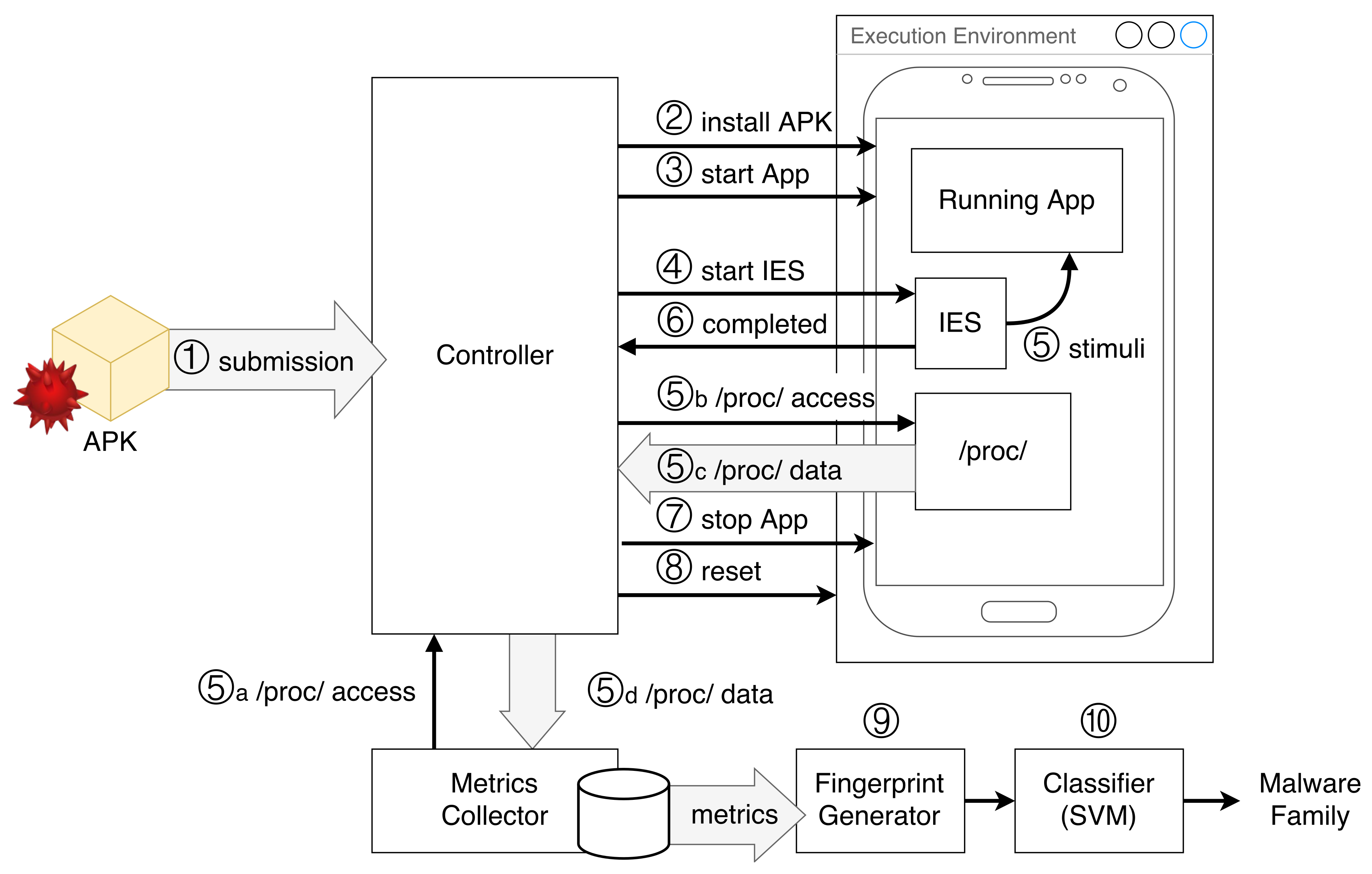
Figure 1 shows an architecture for the implementation of AndroDFA and the expected analysis workflow. Central to the architecture are the Execution Environment, which executes an instance of Android where malware samples are run, and the related Controller, which handles all the interactions with the Execution Environment. First, when the APK of a new malware sample is submitted to the system (Step 1), the Controller is in charge of installing the application into the Execution Environment (Step 2) and launching it (Step 3). During the execution, the app is simulated through a sequence of random input events by the Input Events Simulator (IES) component installed in Android, which is started by the Controller as well (Step 4). During the input stimulation phase (Step 5), the Metrics Collector component accesses the proc file system through the Controller (Steps 5a and 5b). When the IES component notifies the Controller that all input events have been simulated (Step 6), the latter stops the execution of the application (Step 7) and resets the Execution Environment to its initial state (Step 8). Finally, the Fingerprint Generator analyzes the file containing collected metrics to extract the features and generate the fingerprint of the submitted application (Step 9). The fingerprint is then given as input to the SVM classifier, which outputs the family of the malware sample (Step 10).
5.2. Prototype Implementation
To implement the proposed architecture, we leveraged several publicly available third-party tools. We briefly introduce each of them, before discussing how to integrate them within the architecture.
- VirtualBox (https://www.virtualbox.org/) is an open-source hypervisor. It allows virtualizing a guest operating system on a physical machine potentially running a different OS.
- Genymotion (https://www.genymotion.com/) is an Android emulator based on VirtualBox for virtual environment creation. Genymotion provides all the features of a real mobile device, which can be controlled and monitored using VirtualBox’s command-line interface.
- Android Emulator (https://developer.android.com/studio/run/emulator): This is the standard Android Emulator provided with the Android SDK. We built our prototype integrating both Genymotion and Android Emulator to detect if the results depended on the particular emulation environment used.
- Android Debug Bridge (https://developer.android.com/studio/command-line/adb.html) (ADB) is a command-line tool that enables the OS to interact with an Android device and have access to all its resources. ADB also handles installation, as well as the launch and termination of applications.
- UI/Application Exerciser Monkey (https://developer.android.com/studio/test/monkey.html) is a program running on Android devices that can be invoked by the command-line through ADB. It generates stimuli for Android apps by simulating a wide variety of inputs including touches, movements, clicks, system events, and activity launches.
- NOnLinear measures for Dynamical Systems (https://github.com/CSchoel/nolds) (NOLDS) is a Python package that includes different algorithms for one-dimensional time series analysis, including DFA, sample entropy, and the Hurst exponent.
- NumPy (http://www.numpy.org/) is a Python package for scientific computing. We employed it to compute the correlation matrix.
- Scikit-learn [32] is a Python package with several machine learning algorithms for supervised and unsupervised learning, including SVMs.
Tools’ Integration
We implemented the Execution Environment with the Genymotion emulator while ADB served as the Controller component. It handled installing, starting, and stoping applications through appropriate commands.
The UI/Application Exerciser Monkey runs within Android and can simulate input events on any running application. Interactions with Monkey are handled by ADB. It is possible to instruct Monkey to generate a random sequence of events based on a given seed, which makes the sequence deterministically reproducible. In our methodology, we used Monkey to generate the same sequence of input events. It implemented the IES component.
The Metrics Collector component of our architecture was implemented through an ad-hoc Python script, which periodically interacted with ADB. Every sampling period, it processed the files, extracted a sample of the metrics of interest, and stored the samples in a local file.
When all input events were simulated by Monkey, the application was stopped, as well as the virtual machine. The original image of the Android virtual machine was then restored using the VirtualBox command-line tool.
The Fingerprint Generator was implemented as another ad-hoc Python script, which processed the file containing the collected metrics and computed the fingerprint. The features were computed using appropriate functions of the NOLDS and NumPy packages. Finally, the classifier was built and trained through the Scikit-learn package.
The whole workflow described above was completely automated and handled through proper Python scripts. All the software required to reproduce the experiments have been made available on a GitHub repository (https://github.com/lucamassarelli/ANDRODfa).
5.3. Performing Analysis on Real Devices
Although we tested this architecture on virtual devices (emulators), the full pipeline could be easily adapted to use a physical device instead of a virtual one. In our architecture, we used the emulator for two purposes: collecting data during the execution of a malware and restoring the environment after each execution.
As concerns data collection, since we relied on Android Debug Bridge to read data from the device where the malware was executed, there was no difference if the device was emulated or was instead a physical one connected to the USB port. The only requirement for the physical devices was that USB debugging was active. Moreover, the /proc filesystem is mounted in every version of Android (https://source.android.com/devices/architecture/kernel/reqs-interfaces). In recent versions of Android, the /proc filesystem is mounted using a hidepid flag equal to two (https://android.googlesource.com/platform/system/core/+/c39ba5ae32afb6329d42e61d2941d87ff66d92e3). This means that non-privileged users can see information only for the process they own. However, this did not interfere with our solution since we launched the execution of the malware and collected data under the same user.
Finally, restoring the execution environment could be efficiently done on a physical device using tools like the one proposed in [28], which permitted resetting a physical Android device in a few minutes.
6. Experimental Evaluation
We carried out an extensive experimental evaluation to validate our approach. In this section, we discuss the details of the experiments and present the results.
6.1. Datasets
We performed our experiments on two different datasets:
- Drebin dataset [30]: This is a public collection of malware samples collected between 2010 and 2012, which can be used for research purposes. It contains 5560 malicious applications from 179 different families. The Drebin dataset has been widely employed in the related literature [14,18,27,33,34]. Since we compared our solution to DroidScribe, in our experiments, we selected the same families used to evaluate DroidScribe.
- AMD dataset [35]: This is a recent dataset of Android malware labeled by family. It contains 24,553 samples belonging to 71 different families collected until 2017. We selected a subset of this dataset, which includes 13 different families (detailed below), each with more than 20 samples.
6.2. Experiments on the Drebin Dataset
To compare with previous works, we performed different tests with the Drebin dataset. We first ran some experiments to validate our choice of features, then we tested the classification performances of our solution.
6.2.1. Experimental Setup
We ran these experiments on a physical machine with an 8 core Intel Xeon CPU and 16 GB RAM. All software, including the emulator (Genymotion and VirtualBox) and the Python scripts that controlled the workflow of the experiments ran on this machine. The emulator ran an unmodified instance of Android 4.0. We chose this version of Android because it was released during the period in which the samples of the Drebin dataset were collected.
We implemented our methodology as described in Section 5.2. Table 1 reports the complete list of metrics collected by the Metrics Collector component in our experiments. In total, we monitored n = 26 metrics at a sampling frequency of 4 Hz (τ = 0.25 s). In every execution, we generated the same random sequence of simulated input events through Monkey. Furthermore, we configured Monkey to generate each event type with equal probability. In all experiments, we generated S = 10,000 input events. This number was determined after a preliminary study on the stability of the DFA exponent against an increasing number of generated input events. The results of this analysis are discussed in the next section. The stability of the Pearson’s correlation coefficient over resource consumption metrics of Android apps was already studied in [20]. Every experiment was conducted in isolation, as we reset the emulator after every execution.
6.2.2. Time Requirements
To avoid overlap between consecutive Mokey’s inputs, we set a delay of 20 ms between consecutive inputs. For this reason, the execution of a single application with 10,000 inputs required 4 min. Moreover, the average time to restore the emulator to the initial state was one minute. Summing up, each experiment required on average 5 min. Note that experiments were independent; hence, they could be largely parallelized to record data for a large number of applications.
6.2.3. Stability of the DFA exponent
To be meaningful, the fingerprint of an application should remain consistent across different executions. Despite that the conditions of the experiments were kept as constant as possible across different executions, a bit of variability was inevitable, due to multiple exogenous factors, such as network latencies and workload fluctuations. Therefore, we did not expect the fingerprint to remain perfectly constant across different executions. However, it was sufficient for our purposes that the variability was bounded.
As a starting point, we fixed the conditions of the experiments, and we assessed the variance of the DFA exponent across several executions. We selected a random sample of malicious apps, executed each malware 30 times, collected the 26 metrics, and computed the corresponding DFA exponents.
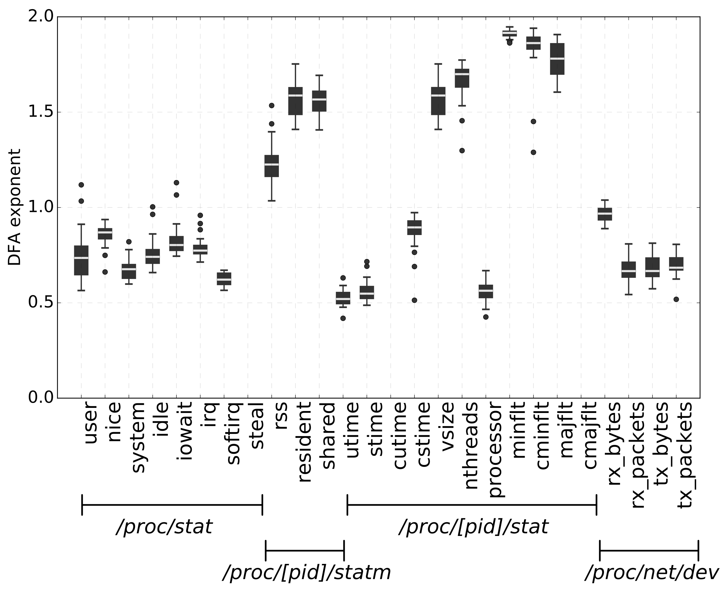
Figure 2 shows the results of these experiments for a single application. For each of the 26 collected metrics, the figure shows the box plot of the corresponding DFA exponent. The bottom and top of each black box represent, respectively, the first and third quartiles of the DFA exponents. The white line within each black box is the median value of the DFA exponent. Whiskers show the interquartile range, and points are outliers. As the figure shows, the DFA exponents were not constant across different executions, but they were characterized by a low variance. This preliminary result supported our intuition that the DFA exponent could be an appropriate feature for the fingerprint.
Subsequently, we assessed the stability of the DFA exponent against the number of simulated input events. We performed several experiments on a random sample of malicious apps with an increasing number of stimuli S, ranging from 2000 to 14,000 with a step of 1000. For each app and value of S, we performed 5 runs, and in each run, we computed the DFA exponents for all metrics. Figure 3 shows the trend of the DFA exponent for 3 selected metrics (user CPU usage, resident set size, number of transmitted packets) with increasing numbers of stimuli. Each point was relative to a metric x and a fixed number of stimuli S. It reports the mean value of the DFA exponents computed for the metric x during the 5 runs in which the number of generated stimuli was S. Bars represent the standard deviations. As the plot shows, the mean value of the DFA exponent appeared to be stable enough across different numbers of generated stimuli. Furthermore, the variance appeared small enough for S from 4000 on. From such results, we decided to fix S = 10,000, as it seemed to be a good trade-off between experiment duration and DFA exponent stability.
6.2.4. SVM Training and Test
In our experiments, we employed a C-SVM with a radial basis function (RBF) kernel as the classifier. To build the training set, we split our dataset of malware: 70% for training, and the remaining 30% for testing. For each training sample, we performed two independent executions (q = 2 (we considered q = 2 a fair trade-off between robustness to noise and length of experiments)) and thus computed two fingerprints. These fingerprints, labeled with the corresponding malware families, constituted the training set. We repeated the same procedure with the test samples to build the test set. We trained the SVM with 5-fold cross-validation and evaluated our approach on the test set. We repeated this procedure for 20 different 70–30% random training/test partitions of the dataset. We evaluated the accuracy of the classifier and finally computed the mean accuracy across these 20 repetitions. During the training phase, we followed the methodology reported in Section 4.2 to determine the best subset of features to employ.
6.2.5. Results
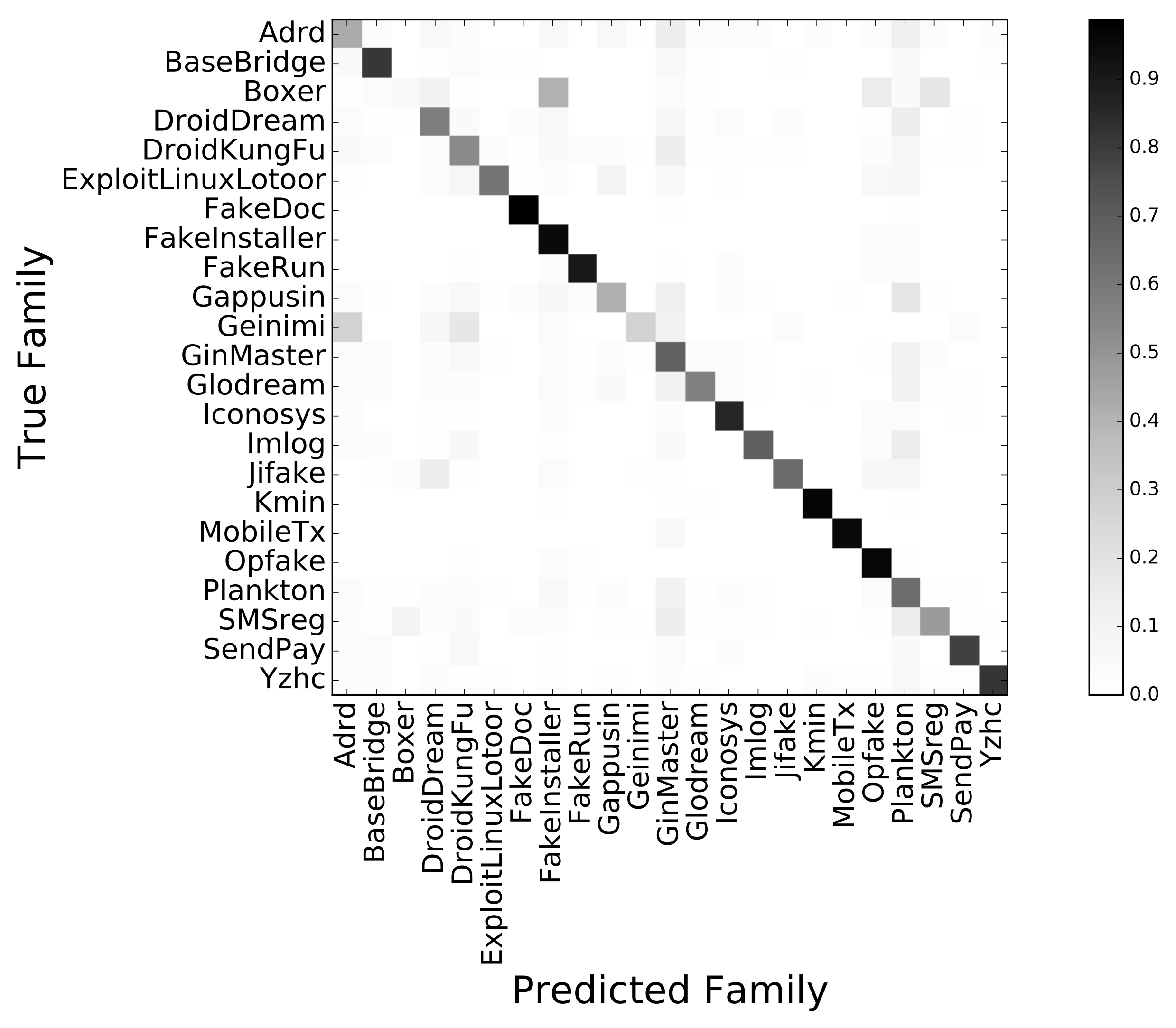
We evaluated our methodology by assessing the accuracy of the classifier through the corresponding confusion matrix M. The generic element of the matrix was the number of samples belonging to class i that was classified as j by the classifier. Figure 4 shows the confusion matrix of our classifier. Each element was normalized in 0–1 by dividing it by the sum of the related row, and the corresponding value was codified with a grayscale for ease of visualization.
To quantify numerically the performance of the classifier, we employed three common metrics: accuracy, recall, and precision. The accuracy is an overall measure of the performance of the classifier. It can be defined with respect to the confusion matrix M as Accuracy = . Precision and recall, instead, are class-related measures and are defined as follows:
After 20 repetitions of our training and test methodology, detailed in the previous section, we obtained a mean value of 82% for the accuracy with a standard deviation of 1%. In Figure 5, we report the mean and standard deviation (depicted as bars and whiskers, respectively) of precision and recall for each malware family. From this figure and the confusion matrix depicted in Figure 4, it was evident that for some families, the classification was nearly perfect (i.e., Fakedoc, MobileTx, Kmin, Opfake). Conversely, two families were misclassified most of the times: Boxer and Geinimi. In particular, the first one was often confused with the FakeInstaller family. By analyzing some samples of this family, we discovered that they contained the same activities of samples from the FakeInstaller family. Moreover, by submitting these samples to VirusTotal (https://www.virustotal.com), we noticed that some antiviruses classified them as Boxer.FakeInstaller. This probably meant that the behavior of the Boxer family samples was very similar to that of the FakeInstaller family. Thus, our classifier was often misled. Instead, most of the samples belonging to the Geinimi family crashed at launch time or during the execution; hence, we were able to collect data only for seven applications of this family. Such a strong imbalance in the proportion of samples in the training set could probably be the reason for the bad performance achieved for this class.
6.2.6. Comparison with DroidScribe
Like DroidScribe, we classified malware into families with an SVM. They achieved 84% accuracy on the Drebin dataset. As already stated, we evaluated the accuracy for 20 different random training/test splittings of the dataset and then computed the mean value. The authors of DroidScribe did not provide enough details about how they split the dataset. Even though this prevented a precise comparison, our results (82% accuracy) were similar to those achieved by DroidScribe. They also presented some results using conformal prediction to improve the accuracy of their approach. In some cases, the confidence on the class output by classifiers (such as SVMs) could be very low. This may reduce the accuracy because the classifier has to choose a single class even though the confidence is only slightly larger than on other classes. Conformal prediction tries to mitigate this problem by letting the classifier output a prediction set (i.e., more classes), instead of a single class. In DroidScribe, they claimed to be able to improve the accuracy from 84% to 94% by using conformal prediction. They achieved 96% accuracy on the malware families for which the confidence was below a certain threshold. However, in this case, the average prediction set size was nine. By including all malware families and using a prediction set size of p > 1 (p was not specified in their paper), the accuracy decreased to 94%. The value of the accuracy has to be necessarily related to the average prediction set size ⟨accuracy, set-size⟩ to be significant. There was no evidence, in general, that ⟨94%, p⟩ was better than ⟨84%, 1⟩. Thus, the two results were not directly comparable. This was why we compared to DroidScribe by only employing the SVM classifier and without using conformal prediction.
6.3. Experiment on the AMD Dataset
We performed experiments also on the AMD dataset since it contained more recent malware samples. These experiments were aimed to show that our solution could perform well also with malware developed for more recent versions of Android OS. For resource constraint reasons, we decided to perform the experiment only over a subset of the AMD dataset. We selected the 13 families with the highest number of samples that were not included in the Drebin dataset. All selected families had more than 20 representative samples, coherently with the experimentation practices introduced in [14]. We discarded all applications that threw any error during their execution. We were able to analyze data from 1626 different APKs. The list of selected families with the number of packages per family is reported in Table 2.
6.3.1. Experimental Setup
We ran these experiments on a machine with an Intel I7 and 32 GB of memory. In this case, rather than the Genymotion emulator used in the previous experiments, we employed the standard Android Emulator shipped together with the Android SDK. We decided to use it to test whether our approach was independent of the emulation platform used. The emulator emulated a Nexus device with an Android 6.0 image. Each package inside our dataset was independently run twice with a different set of 10,000 emulated input actions. The metric collections and the training and testing methodology for this experiment were the same as in the previous one.
6.3.2. Results
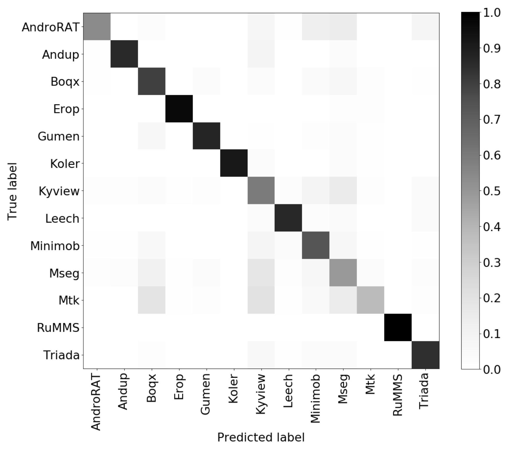
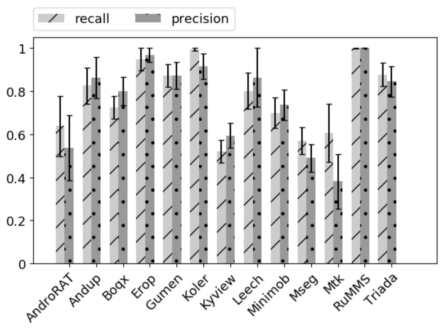
We evaluated the performance of our classification model by computing the overall accuracy, precision, and recall for each class. In Figure 6, we report the confusion matrix obtained after 20 repetitions of the experiments. Each repetition was executed with a different split for training, validation, and test data. The overall mean accuracy was 0.78 with a standard deviation of 0.2. These results were in line with those obtained in the previous experiment with the Drebin dataset. Figure 7 shows the precision and recall values for each malware family. From these results, it was clear that our approach was very robust for detecting malware belonging to the RunMMS or Koler families, while malware from the MSeg or the Mtk families was more difficult to detect with frequent confusion among them. This was probably due to the fact that they showed a very similar behavior since both of them were Trojans released in the same year. In conclusion, we can state that using more recent malware and a different emulation environment did not affect the performance of AndroDFA.
7. Conclusions
In this work, we presented AndroDFA, a novel methodology to classify Android malware into families. This approach was based on dynamic analysis and leveraged resource consumption metrics collected during app execution. Our experimental evaluation showed an accuracy of 82% with malware from the Drebin dataset and the Genymotion emulator. This result was similar to that obtained by DroidScribe, a state-of-the-art work strictly related to ours. Nevertheless, AndroDFA had the following advantages over DroidScribe: (i) it was easier to reproduce because it only employed publicly available tools and did not require any modification to the emulated environment or Android OS, and (ii) by design, it allowed gathering data also on physical devices. The last point was crucial since much of modern malware relies on evasion techniques to hide its malicious behavior on emulated environments. We also investigated how AndroDFA performed when more recent malware (the AMD dataset) and a different emulator (standard Android Emulator) were used. We obtained a 78% accuracy in these experiments.
One of the main weaknesses of this work was the simple interaction with the application under analysis provided by Monkey Tools. The latter was a crucial point since a more human-like interaction would be more likely to trigger the malicious behavior of malware. As future work, it would be interesting to analyze the effect of replacing Monkey Tool with more advanced UI exerciser tools, like [36].
Furthermore, as future work, we aim at improving the accuracy by collecting additional metrics. Moreover, we plan to evaluate our methodology on a more recent and larger malware dataset, which was recently released [35]. Another aspect we intend to investigate is the possibility to integrate on-line learning techniques to update a classifier efficiently over time. Finally, it would be interesting to assess the effectiveness of AndroDFA on physical devices to be more robust against evasion techniques based on the detection of emulated environments. In this regard, we can investigate the possibility to integrate BareDroid [28] in the proposed architecture to reduce analysis overhead time.
Author Contributions
Conceptualization, all authors; methodology, L.M., L.A., C.C., and D.U.; software, L.M.; validation, L.M.; formal analysis, L.M., L.A., C.C., and D.U.; investigation, L.M., L.A., C.C., ad D.U.; resources, all authors; data curation, L.M.; writing, original draft preparation, all authors; writing, review and editing, all authors; visualization, all authors; supervision, L.Q. and R.B.; project administration, L.Q. and R.B.; funding acquisition, L.Q. and R.B. All authors read and agreed to the published version of the manuscript.
Funding
This present work was partially supported by a grant of the Italian Presidency of the Ministry Council and by CINICybersecurity National Laboratory within the project FilieraSicura: Securing the Supply Chain of Domestic Critical Infrastructures from Cyber Attacks (www.filierasicura.it) funded by CISCO Systems Inc. and Leonardo SpA.
Conflicts of Interest
The funders had no role in the design of the study; in the collection, analyses, or interpretation of data; in the writing of the manuscript; nor in the decision to publish the results.
References
- Gartner. Market Share: Final PCs, Ultramobiles and Mobile Phones, All Countries, 4Q16. 2017. Available online: http://www.gartner.com/newsroom/id/3609817 (accessed on 15 June 2020).
- Tam, K.; Feizollah, A.; Anuar, N.B.; Salleh, R.; Cavallaro, L. The evolution of android malware and android analysis techniques. ACM Comput. Surveys (CSUR) 2017, 49, 76. [Google Scholar] [CrossRef] [Green Version]
- Nokia. Nokia Threat Intelligence Report? 2019. 2018. Available online: https://pages.nokia.com/T003B6-Threat-Intelligence-Report-2019.html (accessed on 15 June 2020).
- Symantec. Internet Security Threat Report. 2016. Available online: https://www.symantec.com/content/dam/symantec/docs/reports/istr-21-2016-en.pdf (accessed on 15 June 2020).
- You, I.; Yim, K. Malware obfuscation techniques: A brief survey. In Proceedings of the 5th International Conference on Broadband, Wireless Computing, Communication and Applications, (BWCCA), Fukuoka, Japan, 4–6 November 2010; pp. 297–300. [Google Scholar]
- Pomilia, M. A Study on Obfuscation Techniques for Android Malware. 2016. Available online: https://midlab.diag.uniroma1.it/articoli/matteo_pomilia_master_thesis.pdf (accessed on 15 June 2020).
- Laurenza, G.; Ucci, D.; Aniello, L.; Baldoni, R. An Architecture for Semi-Automatic Collaborative Malware Analysis for CIs. In Proceedings of the 3rd International Workshop on Reliability and Security Aspects for Critical Infrastructure, Toulouse, France, 28 June–1 July 2016. [Google Scholar]
- Ucci, D.; Aniello, L.; Baldoni, R. Survey of machine learning techniques for malware analysis. Comput. Secur. 2019, 81, 123–147. [Google Scholar] [CrossRef] [Green Version]
- Symantec. Internet Security Threat Report; Symantec: Tempe, AZ, USA, 2018. [Google Scholar]
- Peng, C.K.; Buldyrev, S.V.; Havlin, S.; Simons, M.; Stanley, H.E.; Goldberger, A.L. Mosaic Organization of DNA Nucleotides. Phys. Rev. E 1994, 49, 1685–1689. [Google Scholar] [CrossRef] [PubMed] [Green Version]
- Pearson, K. Note on Regression and Inheritance in the Case of Two Parents. Proc. R. Soc. Lond. 1895, 58, 240–242. [Google Scholar]
- Cover, T.M.; Thomas, J.A. Elements of Information Theory; Wiley: Hoboken, NJ, USA, 1991; Volume 4, p. 10. [Google Scholar]
- Jolliffe, I. Principal Component Analysis; Wiley Online Library: Hoboken, NJ, USA, 2002. [Google Scholar]
- Dash, S.K.; Suarez-Tangil, G.; Khan, S.; Tam, K.; Ahmadi, M.; Kinder, J.; Cavallaro, L. Droidscribe: Classifying Android Malware Based on Runtime Behavior. In Proceedings of the 37th Symposium on Security and Privacy Workshops (SPW), San Jose, CA, USA, 22–26 May 2016; pp. 252–261. [Google Scholar]
- Hardstone, R.; Poil, S.S.; Schiavone, G.; Jansen, R.; Nikulin, V.V.; Mansvelder, H.D.; Linkenkaer-Hansen, K. Detrended fluctuation analysis: A scale-free view on neuronal oscillations. Front. Physiol. 2012, 75, 450. [Google Scholar] [CrossRef] [PubMed] [Green Version]
- Ross, B.C. Mutual information between discrete and continuous data sets. PLoS ONE 2014, 9, e87357. [Google Scholar] [CrossRef] [PubMed]
- Mohri, M.; Rostamizadeh, A.; Talwalkar, A. Foundations of Machine Learning; MIT Press: Cambridge, MA, USA, 2012. [Google Scholar]
- Karbab, E.B.; Debbabi, M.; Alrabaee, S.; Mouheb, D. DySign: Dynamic Fingerprinting for the Automatic Detection of Android Malware. In Proceedings of the 11th International Conference on Malicious and Unwanted Software, (MALWARE), Fajardo, PR, USA, 18–22 October 2016; pp. 1–8. [Google Scholar]
- Reina, A.; Fattori, A.; Cavallaro, L. A System Call-centric Analysis and Stimulation Technique to Automatically Reconstruct Android Malware Behaviors. In Proceedings of the 6th European Workshop on Systems Security (EuroSec), Prague, Czech Republic, 14 April 2013. [Google Scholar]
- Shehu, Z.; Ciccotelli, C.; Ucci, D.; Aniello, L.; Baldoni, R. Towards the Usage of Invariant-Based App Behavioral Fingerprinting for the Detection of Obfuscated Versions of Known Malware. In Proceedings of the 10th International Conference on Next Generation Mobile Applications, Security and Technologies (NGMAST), Cardiff, UK, 24–26 August 2016; pp. 121–126. [Google Scholar]
- Bickford, J.; Lagar-Cavilla, H.A.; Varshavsky, A.; Ganapathy, V.; Iftode, L. Security versus energy tradeoffs in host-based mobile malware detection. In Proceedings of the 9th International Conference on Mobile Systems, Applications, and Services, Bethesda, MD, USA, 28 June–1 July 2011; pp. 225–238. [Google Scholar]
- Merlo, A.; Migliardi, M.; Fontanelli, P. On energy-based profiling of malware in android. In Proceedings of the 2014 International Conference on High Performance Computing & Simulation (HPCS), Bologna, Italy, 21–25 July 2014; pp. 535–542. [Google Scholar]
- Caviglione, L.; Gaggero, M.; Lalande, J.F.; Mazurczyk, W.; Urbański, M. Seeing the unseen: Revealing mobile malware hidden communications via energy consumption and artificial intelligence. IEEE Trans. Inf. Forensics Secur. 2015, 11, 799–810. [Google Scholar] [CrossRef] [Green Version]
- Liu, L.; Yan, G.; Zhang, X.; Chen, S. VirusMeter: Preventing Your Cellphone from Spies. In Proceedings of the 12th International Symposium Research in Attacks, Intrusions, and Defenses, (RAID), Saint-Malo, France, 23–25 September 2009; Volume 5758, pp. 244–264. [Google Scholar]
- Kim, H.; Smith, J.; Shin, K.G. Detecting Energy-greedy Anomalies and Mobile Malware Variants. In Proceedings of the 6th International Conference on Mobile Systems, Applications, and Services, (MOBYSYS), Breckenridge, CO, USA, 17–20 June 2008; pp. 239–252. [Google Scholar]
- Amos, B.; Turner, H.; White, J. Applying Machine Learning Classifiers to Dynamic Android Malware Detection at Scale. In Proceedings of the 9th International Wireless Communications and Mobile Computing Conference (IWCMC), Sardinia, Italy, 1–5 July 2013; pp. 1666–1671. [Google Scholar]
- Canfora, G.; Medvet, E.; Mercaldo, F.; Visaggio, C.A. Acquiring and Analyzing App Metrics for Effective Mobile Malware Detection. In Proceedings of the 2016 International Workshop on Security and Privacy Analytics, New Orleans, LA, USA, 11 March 2016; pp. 50–57. [Google Scholar]
- Mutti, S.; Fratantonio, Y.; Bianchi, A.; Invernizzi, L.; Corbetta, J.; Kirat, D.; Kruegel, C.; Vigna, G. BareDroid: Large-scale Analysis of Android Apps on Real Devices. In Proceedings of the 31st Computer Security Applications Conference, (ACSAC), Los Angeles, CA, USA, 7–11 December 2015; pp. 71–80. [Google Scholar]
- Massarelli, L.; Aniello, L.; Ciccotelli, C.; Querzoni, L.; Ucci, D.; Baldoni, R. Android malware family classification based on resource consumption over time. In Proceedings of the 2017 12th International Conference on Malicious and Unwanted Software (MALWARE), Fajardo, Puerto Rico, 11–14 October 2017; pp. 31–38. [Google Scholar]
- Arp, D.; Spreitzenbarth, M.; Hubner, M.; Gascon, H.; Rieck, K.; Siemens, C. Drebin: Effective and Explainable Detection of Android Malware in Your Pocket. In Proceedings of the 21st Network and Distributed System Security Symposium, (NDSS), San Diego, CA, USA, 23–26 February 2014. [Google Scholar]
- Guyon, I.; Elisseeff, A. An Introduction to Variable and Feature Selection. J. Mach. Learn. Res. 2003, 3, 1157–1182. [Google Scholar]
- Pedregosa, F.; Varoquaux, G.; Gramfort, A.; Michel, V.; Thirion, B.; Grisel, O.; Blondel, M.; Prettenhofer, P.; Weiss, R.; Dubourg, V.; et al. Scikit-learn: Machine Learning in Python. J. Mach. Learn. Res. 2011, 12, 2825–2830. [Google Scholar]
- Gonzalez, H.; Stakhanova, N.; Ghorbani, A.A. DroidKin: Lightweight Detection of Android Apps Similarity. In Proceedings of the 10th International Conference on Security and Privacy in Communication Networks (SECURECOMM), Beijing, China, 24–26 September 2014; pp. 436–453. [Google Scholar]
- Suarez-Tangil, G.; Dash, S.K.; Ahmadi, M.; Kinder, J.; Giacinto, G.; Cavallaro, L. DroidSieve: Fast and Accurate Classification of Obfuscated Android Malware. In Proceedings of the 7th Conference on Data and Application Security and Privacy (CODASPY), Scottsdale, AZ, USA, 22–24 March 2017; pp. 309–320. [Google Scholar]
- Wei, F.; Li, Y.; Roy, S.; Ou, X.; Zhou, W. Deep ground truth analysis of current android malware. In Proceedings of the 14th International Conference on Detection of Intrusions and Malware, and Vulnerability Assessment, (DIMVA), Bonn, Germany, 6–7 July 2017; pp. 252–276. [Google Scholar]
- Gianazza, A.; Maggi, F.; Fattori, A.; Cavallaro, L.; Zanero, S. Puppetdroid: A user-centric ui exerciser for automatic dynamic analysis of similar android applications. arXiv 2014, arXiv:1402.4826. [Google Scholar]
Figure 1.
Proposed architecture and workflow for AndroDFA. IES, Input Events Simulator.

Figure 2.
Box plot of the DFA exponents obtained from 30 independent executions for a randomly sampled malicious app, for each of the 26 metrics.
Figure 2.
Box plot of the DFA exponents obtained from 30 independent executions for a randomly sampled malicious app, for each of the 26 metrics.

Figure 3.
Stability of the DFA exponent for three different metrics: user CPU, resident set size, and transmitted packets.
Figure 3.
Stability of the DFA exponent for three different metrics: user CPU, resident set size, and transmitted packets.

Figure 4.
Normalized confusion matrix of the SVM classifier.

Figure 5.
Precision and recall values for all 23 classes.

Figure 6.
Confusion matrix for the experiment over the AMD dataset.

Figure 7.
Precision and recall for each class in the AMD dataset.


Table 1.
Monitored metrics from the proc file system.
| File (/proc/) | Metric | Description |
|---|---|---|
| [pid]/statm | vss | Total program size |
| rss | Resident set size | |
| shared | Shared pages | |
| rmsize | Size of resident file mappings | |
| net/dev | Rx_packets | Packets received over WiFi |
| Rx_bytes | Bytes received over WiFi | |
| Tx_packets | Packets sent over WiFi | |
| Tx_bytes | Bytes sent over WiFi | |
| stat | u_cpu | CPU time in user mode |
| s_cpu | CPU time in kernel mode | |
| i_cpu | CPU idle time | |
| io_cpu | CPU time in I/O wait | |
| irq_cpu | CPU time servicing interrupt | |
| sirq_cpu | CPU time servicing softirq | |
| st_cpu | CPU time spent in other operating systems | |
| [pid]/stat | utime | Time spent by the process in user mode |
| stime | Time spent by the process in kernel mode | |
| cutime | Time spent by the process waiting for children scheduled in user mode | |
| cstime | Time spent by the process waiting for children scheduled in kernel mode | |
| num_threads | Number of threads | |
| processor | CPU number last executed on | |
| min | Number of minor faults the process made that do not require loading a memory page from disk | |
| cmin | Number of minor faults that the process’s waited-for children made | |
| maj | Number of major faults the process made that required loading a memory page from disk | |
| cmaj | Number of major faults that the process’s waited-for children made |
Table 2.
Selected package per family for the AMD dataset.
| Family | No. of Packages |
|---|---|
| Mseg | 195 |
| Minimob | 153 |
| Andup | 40 |
| Leech | 55 |
| Erop | 40 |
| Kyview | 155 |
| Mtk | 59 |
| Koler | 62 |
| AndroRAT | 31 |
| RuMMS | 366 |
| Boqx | 191 |
| Triada | 152 |
© 2020 by the authors. Licensee MDPI, Basel, Switzerland. This article is an open access article distributed under the terms and conditions of the Creative Commons Attribution (CC BY) license (http://creativecommons.org/licenses/by/4.0/).
Share and Cite
MDPI and ACS Style
Massarelli, L.; Aniello, L.; Ciccotelli, C.; Querzoni, L.; Ucci, D.; Baldoni, R. AndroDFA: Android Malware Classification Based on Resource Consumption. Information 2020, 11, 326. https://0-doi-org.brum.beds.ac.uk/10.3390/info11060326
AMA Style
Massarelli L, Aniello L, Ciccotelli C, Querzoni L, Ucci D, Baldoni R. AndroDFA: Android Malware Classification Based on Resource Consumption. Information. 2020; 11(6):326. https://0-doi-org.brum.beds.ac.uk/10.3390/info11060326
Chicago/Turabian StyleMassarelli, Luca, Leonardo Aniello, Claudio Ciccotelli, Leonardo Querzoni, Daniele Ucci, and Roberto Baldoni. 2020. "AndroDFA: Android Malware Classification Based on Resource Consumption" Information 11, no. 6: 326. https://0-doi-org.brum.beds.ac.uk/10.3390/info11060326
Note that from the first issue of 2016, this journal uses article numbers instead of page numbers. See further details here.