SVD++ Recommendation Algorithm Based on Backtracking

Abstract

Collaborative filtering (CF) has successfully achieved application in personalized recommendation systems. The singular value decomposition (SVD)++ algorithm is employed as an optimized SVD algorithm to enhance the accuracy of prediction by generating implicit feedback. However, the SVD++ algorithm is limited primarily by its low efficiency of calculation in the recommendation. To address this limitation of the algorithm, this study proposes a novel method to accelerate the computation of the SVD++ algorithm, which can help achieve more accurate recommendation results. The core of the proposed method is to conduct a backtracking line search in the SVD++ algorithm, optimize the recommendation algorithm, and find the optimal solution via the backtracking line search on the local gradient of the objective function. The algorithm is compared with the conventional CF algorithm in the FilmTrust, MovieLens 1 M and 10 M public datasets. The effectiveness of the proposed method is demonstrated by comparing the root mean square error, absolute mean error and recall rate simulation results.

1. Introduction

As fueled by the advancement of electronic information and the booming of the smart business industry, personalized recommendations are critical to e-commerce and e-books. Over the past few years, personalized recommendations have been the hotspots of business and academic research [1]. In personalized recommendation, recommender systems commonly comply with CF [2], depending on user past behavior. CF analyzes the relationships between users and interdependencies of products to identify emerging user–item associations. Two main areas of CF are neighborhood methods and latent factor models. The core of the neighborhood method is to calculate the relationship between items or users. The item-oriented method evaluates the user’s preference for the item based on the same user’s rating of neighbors. The latent factor model is another method to try to explain the rating by describing the 20 to 100 factors inferred by the scoring model. Recently, SVD models have been extensively applied for their high accuracy and scalability [3,4,5]. The Funk SVD [6] and Bias SVD [7] algorithms introduce biasing factors, and subsequently the recommended algorithm to optimize SVD++ [8] based on both has achieved broad application for its implicit feedback, reduced dimensionality, and high prediction accuracy.

However, in the emerging big data era, the SVD++ algorithm exhibits significant defects (i.e., low computational efficiency). In the recommendation, the algorithm should be iterated too many times to achieve the optimal solution.

In this study, a novel method is developed to accelerate the computational of the SVD++ algorithm. By conducting the backtracking line search [9,10], the optimal solution is found [11] on the local gradient of the objective function till the objective function is identified to decrease as expected.

In Section 2, the recommendation system is reviewed. In Section 3, the algorithm is presented. Next, Section 4 analyzes the simulation results. Finally, the conclusion is drawn based on the received packets.

2. Recommendation System

2.1. SVD Recommendation Algorithm

The recommendation system aims to provide product information and suggestions to customers via the e-commerce website. On that basis, the system attempts to help users determine what products should be purchased, and to simulate sales personnel to help customers complete the purchase [12,13]. The personalized recommendation system refers to a massive data mining-based advanced information retrieval platform. It will recommend information and products to interested users based on their scenarios and the characteristics of users.

SVD++ refers to an optimized algorithm based on SVD [14]. SVD is a common matrix decomposition technique; it can effectively extract algebraic features. SVD in CF is mainly to analyze the preference of the scorer for each factor and the extent to which the film contains each factor in the existing scoring scenario. Lastly, the data are analyzed in turn to achieve the predicted result.

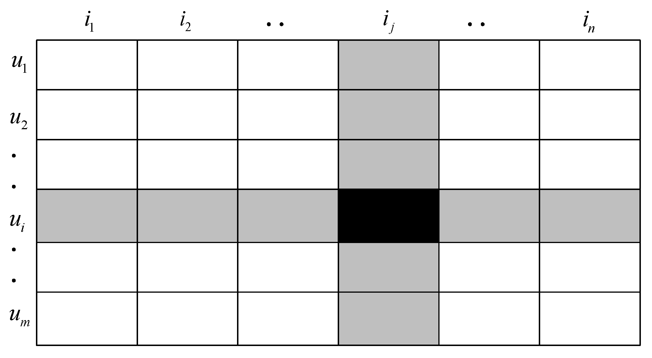
It is assumed that there are $m$ users, $n$ items, and the user’s rating matrix $R\in R^{m\ast n}$ for the item, where the $R$ matrix is sparse, and $R_{i,j}$ denotes the user $i$’s score for item $j$, as shown in Figure 1.

Each of the above lines represents a user, and each column denotes an item. This is the user–item matrix, which is highly sparse (i.e., the number of ratings is known as a small part of the total, which is also the practical corresponding). The scoring matrix $U$ can be decomposed into two matrix multiplications.

$$\begin{array}{ll}U& =\left[\begin{array}{l}{u}_{11}\hspace{1em}\cdots \hspace{1em}{u}_{1k}\\ ⋮\hspace{1em}\hspace{1em}\ddots \hspace{1em}⋮\\ u_{m1}\hspace{1em}\cdots \hspace{1em}{u}_{mk}\end{array}\right] \times \left[\begin{array}{l}{i}_{11}\hspace{1em}\cdots \hspace{1em}{i}_{1n}\\ ⋮ \hspace{1em}\ddots \hspace{1em}⋮\\ i_{k1}\hspace{1em}\cdots \hspace{1em}{i}_{kn}\end{array}\right]\\ & =\left[\begin{array}{l}{p}_1^T\\ ⋮\\ p_m^T\end{array}\right] \times \left[q_1\hspace{1em}\cdots \hspace{1em}{q}_n\right]\end{array}$$

(1)

This matrix decomposition method is reflected in CF:

$$R_{U\times I}=P_{U\times K}{Q}^T{}_{K\times I}$$

(2)

where $U$ is the number of users, $I$ is the number of commodities, $K$ is the number of potential factors. Since the scoring matrix $R$ is sparse, SVD trains the matrix $P$ and $Q$ by decomposing the known data in the matrix, then the unknown score can be obtained by the product of $P$ and $Q$, which is the prediction matrix:

$${\widehat{r}}_{ui}=q_{ki}^T{p}_{uk}=p_{uk}^T{q}_{ki}$$

(3)

where ${\widehat{r}}_{ui}$ denotes the score of user $u$ for item $i$; $p_u\in R^f$ represents the implicit factor matrix mapped by the user to the f-dimension, the degree of preference of user $u$ for factor $k$, $q_i\in R^f$ represents the implicit factor matrix of item mapping to the f-dimension, for item $i$, the degree on the factor $k$. In other words, the two decomposed matrices refer to the user matrix and the item matrix, and the user’s score on the item is the dot product of the vector.

Given this solution to SVD, it is possible to solve the square sum of the minimum error between the actual value and the predicted value. The values of the matrix $P_{U\times K}$ and $Q_{K\times I}$ can best fit $R$. For the actual score value $r_{ui}$, to learn the latent vectors $p_{uk}$ and $q_{ki}$, the maximum likelihood method is to minimize the square error of known ratings.

$${\displaystyle \sum _{u,i}{e}^2{}_{ui}}=\underset{q_i,p_u}{\min }{\displaystyle {\sum }_{u,i}(r_{ui}-{\displaystyle \sum _{k=1}^K{p}_{uk}{q}_{ki}^T{)}^2}}$$

(4)

2.2. RSVD and SVD++ Recommendation Algorithm

SVD has achieved broad application in terms of data decomposition, but in case of sparse data, the observed set $R$ of ratings is small, which will be overfitting. When the actual data are predicted, the effect is far worse than the training data. Over-reliance on the characteristics of the existing training data set can cause overfitting. In the process of model parameter fitting, since the training data contain sampling errors, the complicated model will also fit the sampling errors during training [15].

Common methods are cross-validation, pruning, regularization, etc. to solve overfitting. Regularization is the most common solution for overfitting in machine learning. Regularization terms are added to the loss function to punish the parameters of the model, thereby reducing the complexity of the model.

Therefore, on the basis of the SVD algorithm, add $\frac{\lambda }{2}(P^2+Q^2)$ regularization term in Equation (4) with $\lambda >0$ is regularization parameter. Adding the regularized SVD algorithm is the RSVD algorithm.

$${\displaystyle \sum _{u,i}{e}^2{}_{ui}}=\underset{q_i,p_u}{\min }{\displaystyle {\sum }_{u,i}(r_{ui}-{\displaystyle \sum _{k=1}^K{p}_{uk}{q}_{ki}^T{)}^2}}+\frac{\lambda }{2}{\displaystyle \sum _u{\left|p_u\right|}^2}+\frac{\lambda }{2}{\displaystyle \sum _i{\left|q_i\right|}^2}$$

(5)

By introducing the mentioned implicit feedback to optimize the RSVD algorithm, the SVD++ algorithm is developed, and user history browsing data and historical score data are added as novel parameters. The predicted score Equation (3) is as follows:

$${\widehat{r}}_{ui}=\mu +b_i+b_u+q_i^T(p_u+{\left|N(u)\right|}^{-\frac{1}{2}}{\displaystyle \sum _{j\in N(u)}{y}_j})$$

(6)

where: $\mu$ denotes the global mean; $b_i$ is the offset vector of the item; $b_u$ is the user offset vector; $q_i$ is the item i feature vector; $p_u$ is the feature vector of the user u score; $\left|N(u)\right|$ is the user $u$’s behavior item set; $y_j$ is the item implicit feedback expressed by $j$; ${\left|N(u)\right|}^{-\frac{1}{2}}{\displaystyle \sum _{j\in N(u)}{y}_j}$ is the eigenvector of the user $u$ implicit feedback; $p_u+{\left|N(u)\right|}^{-\frac{1}{2}}{\displaystyle \sum _{j\in N(u)}{y}_j}$ here denotes the feature vector of the user $u$ that introduces implicit feedback.

2.3. Latent Factor Model and Loss Function

To be specific, the publication of $b_i$ and $b_u$ is expressed as follows:

$$b_i=\frac{{\displaystyle \sum u\in R(i)(r_{ui}-\mu )}}{\alpha +\left|R(i)\right|}$$

(7)

$$b_u=\frac{{\displaystyle \sum i\in R(u)(r_{ui}-\mu -b_i)}}{\beta +\left|R(u)\right|}$$

(8)

With the mean square error as the loss function, ${(r_{ui}-{\widehat{r}}_{ui})}^2$ is expected to be as small as possible [16]. ${\widehat{r}}_{ui}$ refers to the predicted score. If the combination of all items and samples is considered, this yields:

$$\min {{\displaystyle \sum _{i,u}(r_{ui}-{\widehat{r}}_{ui})}}^2$$

(9)

Since $r_{ui}$ is known, it is only required to ask for the values in the ${\widehat{r}}_{ui}$ corresponding to the minimum value of the above formula and to finally find the $p_u$ and $q_i$. Subsequently, the blank score can be assessed in any $R^{m\ast n}$. To prevent overfitting, an L2 regularization term is added, and it yields:

$$\min {{\displaystyle \sum _{i,u}\left[r_{ui}-\mu -b_i-b_u-q_i^T(p_u+{\left|N(u)\right|}^{-\frac{1}{2}}{\displaystyle \sum _{j\in N(u)}{y}_j})\right]}}^2+\lambda ({\Vert b_u\Vert }^2+{\Vert b_u\Vert }^2+{\Vert p_u\Vert }^2+{\Vert q_i\Vert }^2+{{\displaystyle \sum _{j\in N(u)}\Vert y_j\Vert }}^2)$$

(10)

where $\lambda$ denotes the regularization coefficient. Overall, two methods can be adopted to solve this objective function (i.e., namely the iterative least squares algorithm and the gradient descent method). In the iterative least squares method, the $p_u$ optimization is fixed first; subsequently, the $q_i$ optimization $p_u$ is fixed, and the update is alternated. The algorithm is overly redundant and difficult to implement under large data; thus, the gradient descent method is used. It is assumed that the minimum value of function $f(x)$ is solved. First, an initial point is taken, the gradient of the point is calculated, and next the independent variable is updated with the direction of the gradient. Under the $k$ iteration value of $x^{(k)}$, the $k+1$ iteration value is expressed as:

$$x^{(k+1)}=x^{(k)}-\alpha \nabla f(x^{(k)})$$

(11)

where $\alpha$ is termed as the step size or learning efficiency, representing the size of the change in the iteration of the argument [17]. The independent variable is constantly updated with the above formula until the function value is altered slightly or stops when the maximum number of iterations is reached. Then, the independent variable is updated to the minimum value of the function. To avoid the local optimal solution, the random gradient descent method is adopted on the whole. By computing each parameter’s partial derivatives of the loss function, the iterative formula can be effectively solved. For a given training case $r_{ui}$, the parameters are modified by moving in the opposite direction of the gradient, and it yields:

$$\begin{array}{l}{e}_{ui}\leftarrow r_{ui}-{\widehat{r}}_{ui}\\ b_i\hspace{0.17em}\leftarrow b_i+\gamma (e_{ui}-\lambda b_i)\\ b_u\hspace{0.17em}\leftarrow b_u+\gamma (e_{ui}-\lambda b_u)\\ p_u\hspace{0.17em}\leftarrow p_u+\gamma (e_{ui}·q_i-\lambda p_u)\\ q_i\hspace{0.17em}\leftarrow q_i+\gamma (e_{ui}·(p_u+{\left|N(u)\right|}^{-\frac{1}{2}}{\displaystyle \sum _{j\in N(u)}{y}_j})-\lambda q_i)\\ y_j\hspace{0.17em}\leftarrow y_j+\gamma (e_{ui}·{\left|N(u)\right|}^{-\frac{1}{2}}·q_i-\lambda q_i)\end{array}$$

(12)

3. Backtracking Based SVD++ Model

In the SVD++ algorithm training, the fixed step size is commonly employed when solving the minimum value. For the selection, under the extremely large value, though it can reach the minimum value efficiently, it cannot reach the optimal solution based on a few iterations, or even Convergence, so the optimal solution cannot be obtained. If the value is overly small, though the optimal solution can be reached, there are considerable iterations, and the rate of decline is too slow, thereby taking much time and low efficiency.

Therefore, this study proposes to conduct a backtracking line search. Backtracking line search is a search scheme to determine the maximum amount of movement along a given direction of descent. Starting with an estimate from when the step value along the descending direction is relatively large, the step size is iteratively reduced till the objective function is identified to be sufficiently reduced based on the gradient [18]. The following judgments should be satisfied:

$$f(x-\gamma \nabla f(x))>f(x)-\alpha \gamma {\Vert \nabla f(x)\Vert }_2^2$$

(13)

$$\gamma =\beta \ast \gamma$$

(14)

$0<\beta \le 1$, $0<\alpha \le 1/2$ after the backtracking condition is satisfied, the step size is updated, so the objective function is constantly updated in the falling direction [19]. In the SVD++ algorithm, the gradient descent introduces the backtracking, so this study proposes an optimized backtracking algorithm (i.e., BLS-SVD++ algorithm). If the backtracking condition is not met, it yields:

$$\gamma =\eta \ast \gamma$$

(15)

where $0<\eta \le 1$. With the increase in the number of iterations, the step size gradually shrinks, and the results are more accurate. If only the backtracking is satisfied, the loop will jump out promptly without satisfying the backtracking condition, which will significantly reduce the accuracy of the result. Since the initial value of the backtracking line search is large, the descent speed is fast at the beginning and the backtracking line search can easily jump out of the loop shortly. Then, the minimum value of the objective function is not the optimal solution, whereas it is because the backtracking condition is not satisfied. Adding this formula reduces the step size when the backtracking condition is not met till the backtracking condition is met, or the number of iterations is reached. Accordingly, the iterative result exhibits higher accuracy since the initial step size is larger, so the initial time is more efficient than the random gradient drop. In the later part of the iteration, by adding the Equation (11), the backtracking line search is solved since the gradient descent is not satisfied. The backtracking line search jumps out of the loop, and a smaller step size can be exploited to yield a more accurate optimal solution.

Decreasing the value of the objective function is the most expected result. If the search step is too large, the objective function may jump out of the loop directly. If the search step size is too small, the objective function may continuously iterate on a value, making it difficult to find the optimal solution.

In the added function $f(x_k-\gamma d_k)$, on a certain $x$, after the search direction $d_k$ is determined, then, it only needs to find a suitable step size. Therefore, this is a nonlinear function, with $\gamma$ as its independent variable. If Equation (13) is satisfied, then the following formula will be satisfied:

$$f(x_k-{\gamma }_k{d}_k))\le f(x_k)-{\alpha }_1{\gamma }_k\nabla f{(x_k)}^T{d}_k$$

(16)

$$f(x_k-{\gamma }_k{d}_k))\le f(x_k)-{\alpha }_2{\gamma }_k\nabla f{(x_k)}^T{d}_k$$

(17)

where the inequality is Taylor expansion on the left, it yields:

$$f(x_k-{\gamma }_k{d}_k)=f(x_k)-{\gamma }_k{g}_k^T{d}_k+o({\gamma }_k)$$

(18)

Since $g_k^T{d}_k<0$, $f(x_k)-{\lambda }_k\rho g_k^T{d}_k<f(x_k)$. Then this objective function will inevitably decrease, and the learning rate will be changed adaptively. First, the gradient descent is performed with a larger value step size, so that the objective function can be reduced faster during the initial iteration, and it is quickly dipped to the vicinity of the optimal solution. As the number of iterations increases, the learning rate gradually decreases, and the optimal solution can be searched with a small learning rate, so that the optimal solution can be reached in fewer iterations.

In SVD, decomposing an $m\ast n$ matrix $R_{mn}$ needs to be decomposed into an $m\ast m$ matrix $P_{mm}$ and an $m\ast n$ matrix $Q_{mn}$. The two decomposition matrices do not reduce the dimensions of the original matrix much. The multiplication and iteration of the two matrices result in a time complexity of SVD of $O(m{n}^2+n{m}^2)$. According to the definition of time complexity, the time of SVD can be obtained and the complexity is $O(n^3)$.

It is known that RSVD and SVD++ algorithms are obtained by adding regularization and implicit vectors through the SVD algorithm. Even if the implicit feedback of users and items is added, the prediction score matrix acquisition does not need to rely too much on matrix decomposition matrix $P_{mm}$ and matrix $Q_{mn}$, but the acquisition of implicit vectors still requires m times of user implicit vector acquisition and acquisition in matrix $R_{mn}$ n times item implicit vector acquisition. Therefore, RSVD and SVD++ have the same time complexity as SVD, which is $O(n^3)$. The BLS-SVD++ algorithm proposed in this paper adds backtracking judgment in the loop process, and does not add the loop and the time complexity is $O(n^3+b)$, that is, in the worst case, the time complexity is $O(n^3)$. That is the same time complexity as the SVD++ algorithm.

After ensuring that the loss function decreases, Equation (14) is added to make the objective function search for more optimal advantages in the gradient descent process. Because the initial value of the step size is large, the decline rate is fast at the beginning and it is easy to jump out of the loop in a short time, so that the final non-optimal solution is solved. Therefore, Equation (15) is added to reduce the step size and ensure the final result is more accurate.

Therefore, the BLS-SVD++ algorithm obtains the optimal value through rapid gradient descent under the same time complexity, reducing the total number of algorithm iterations to improve the overall efficiency.

The specific algorithm flow is written in Algorithm 1.

Algorithm 1 BLS-SVD++

Input: Training set u-train. Initialization: Iterations step, $\gamma =0.05$, $\lambda =0.1$, $\alpha =0.25$, $\beta =0.8$, $\eta =0.9$, average value $\mu$, scoring matrix $R^{m\ast n}$, $bu\left[uid\right]=0$, $bi\left[iid\right]=0$, $pu\left[uid\right]=random(0,0.1)$, $qi\left[iid\right]=random(0,0.1)$, $y\_u+=y[i]$ Iteration: For step in rang(steps):  $$\begin{gathered} bu[uid]\hspace{0.17em}+=\gamma \ast (eui-\lambda \ast bu[uid]) \\ bi[iid]\hspace{0.17em}+=\gamma \ast (eui-\lambda \ast bi[iid]) \\ pu[uid]\hspace{0.17em}+=\gamma \ast (eui\hspace{0.17em}\ast \hspace{0.17em}qi[iid]-\lambda \ast pu[uid]) \\ \begin{array}{l}qi[iid]\hspace{0.17em}+=\gamma \ast (eui\hspace{0.17em}\ast \hspace{0.17em}(pu[uid]\\ +y\_u/sqrt\_N(u))-\lambda \ast qi[iid])\end{array} \end{gathered}$$ For j in self.u_dict[uid]:  $y[j]+=\gamma \ast (eui\ast qi[j])/sqrt\_N(u)-\lambda \ast qi[j])$ If $\begin{array}{l}f(eui,bu[uid],bi[iid],pu[uid]-\gamma \ast \\ f\_grad(eui,pu[uid]),qi[iid],y[j])>\\ f(eui,bu[uid],bi[iid],pu[uid],qi[iid],y[j])-\\ \alpha \ast \gamma \ast f\_grad(eui,pu[uid])**2\\ \gamma =\beta \ast \gamma \end{array}$ $\gamma =\eta \ast \gamma$ end Output: MAE\RMSE and Recall

4. Experimental Results and Analysis

4.1. Lab Environment

This study uses the FilmTrust, MovieLens site 1 M and 10 M datasets as experimental datasets, covering 35,497 ratings from 1508 users on 2071 movies, 6000 users’ ratings of 4000 movies and 72,000 users, and 10 million ratings and 100,000 tags for 10,000 movies. The FilmTrust dataset has a rating range of 0.5 to 4, where 0.5 is the lowest grade, and 4 is at the highest level. The MovieLens dataset’s rating is split into 1–5 grades, where 1 is the lowest grade, and 5 is at the highest level. Each user in the dataset scores at least 20 items, and the selected data set is divided into training sets and test sets by 80% and 20%.

4.2. Evaluation Metrics

To ensure the accuracy of the recommendation results, the absolute mean error (MAE), root mean square error (RMSE) and recall rate act as the recommended system evaluation indicators. The recommended quality can be measured intuitively. The smaller the values of MAE and RMSE, the greater the value of the recall rate will be [20,21,22], and the higher the accuracy will be. The expression is as follows:

$$MAE={\displaystyle \sum _{r_{ui}\in T_{test}}\frac{\left|{\widehat{r}}_{ui}-r_{ui}\right|}{N}}$$

(19)

$$RMSE=\sqrt{{\displaystyle \sum _{r_{ui}\in T_{test}}\frac{{({\widehat{r}}_{ui}-r_{ui})}^2}{N}}}$$

(20)

$$recall=\frac{{\displaystyle {\sum }_{u\in U}\left|R(u)\cap T(u)\right|}}{{\displaystyle {\sum }_{u\in U}\left|T(u)\right|}}$$

(21)

where: N denotes the number of samples in the test set; $R(u)$ is the recommended list generated by the recommendation system for the user on the test set; $T(u)$ is the user’s favorite item on the test set.

4.3. Evaluating of Result

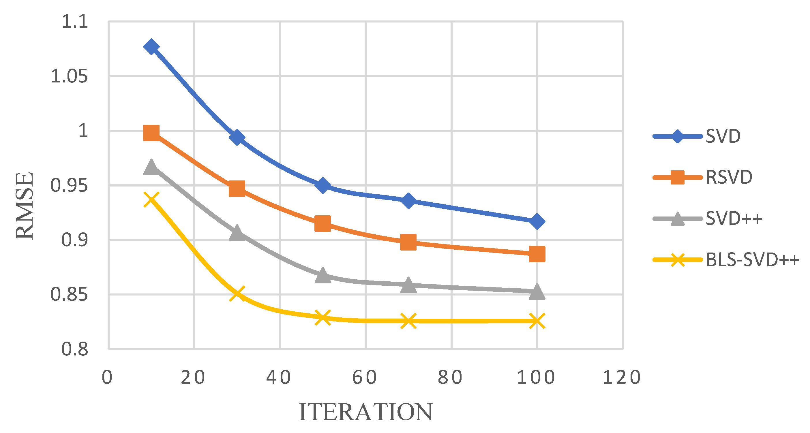
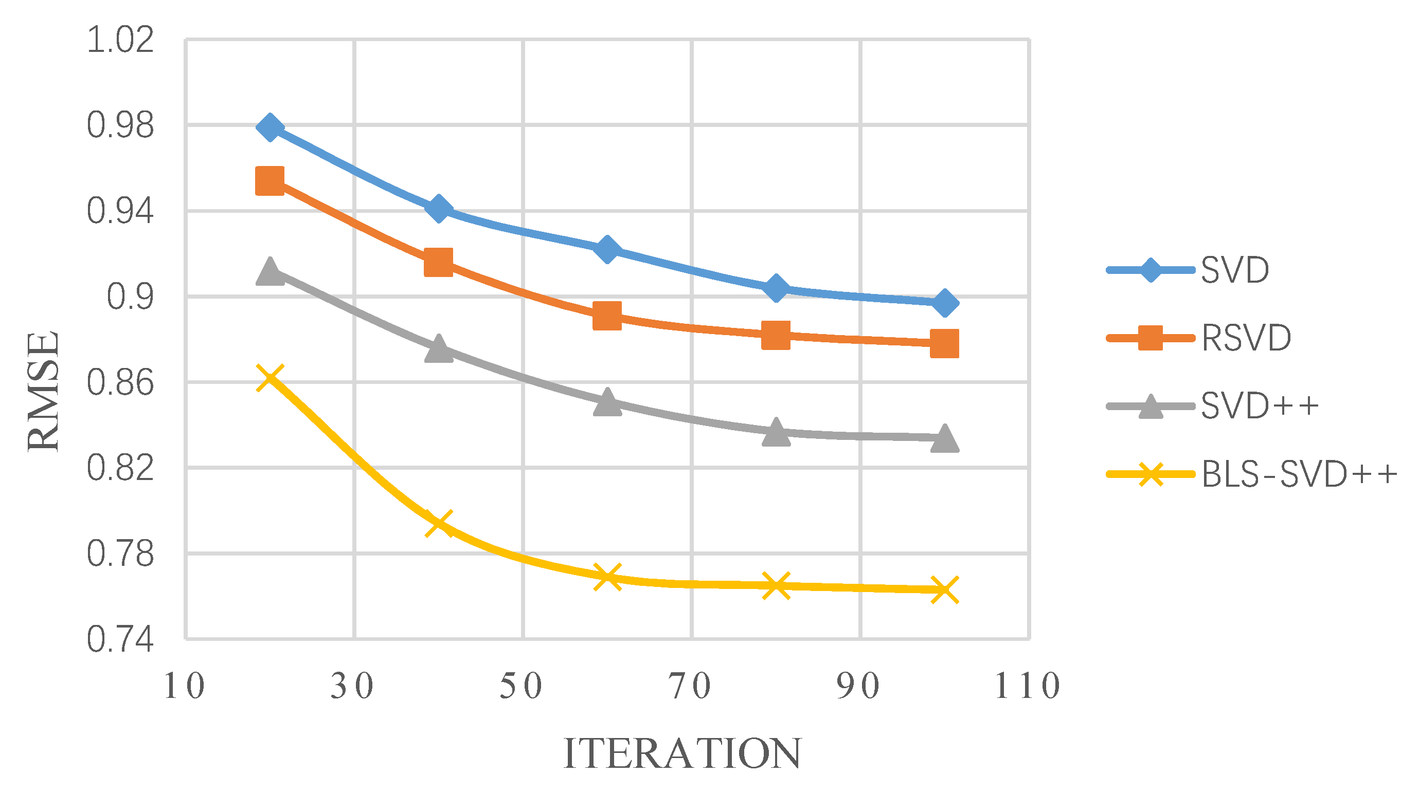
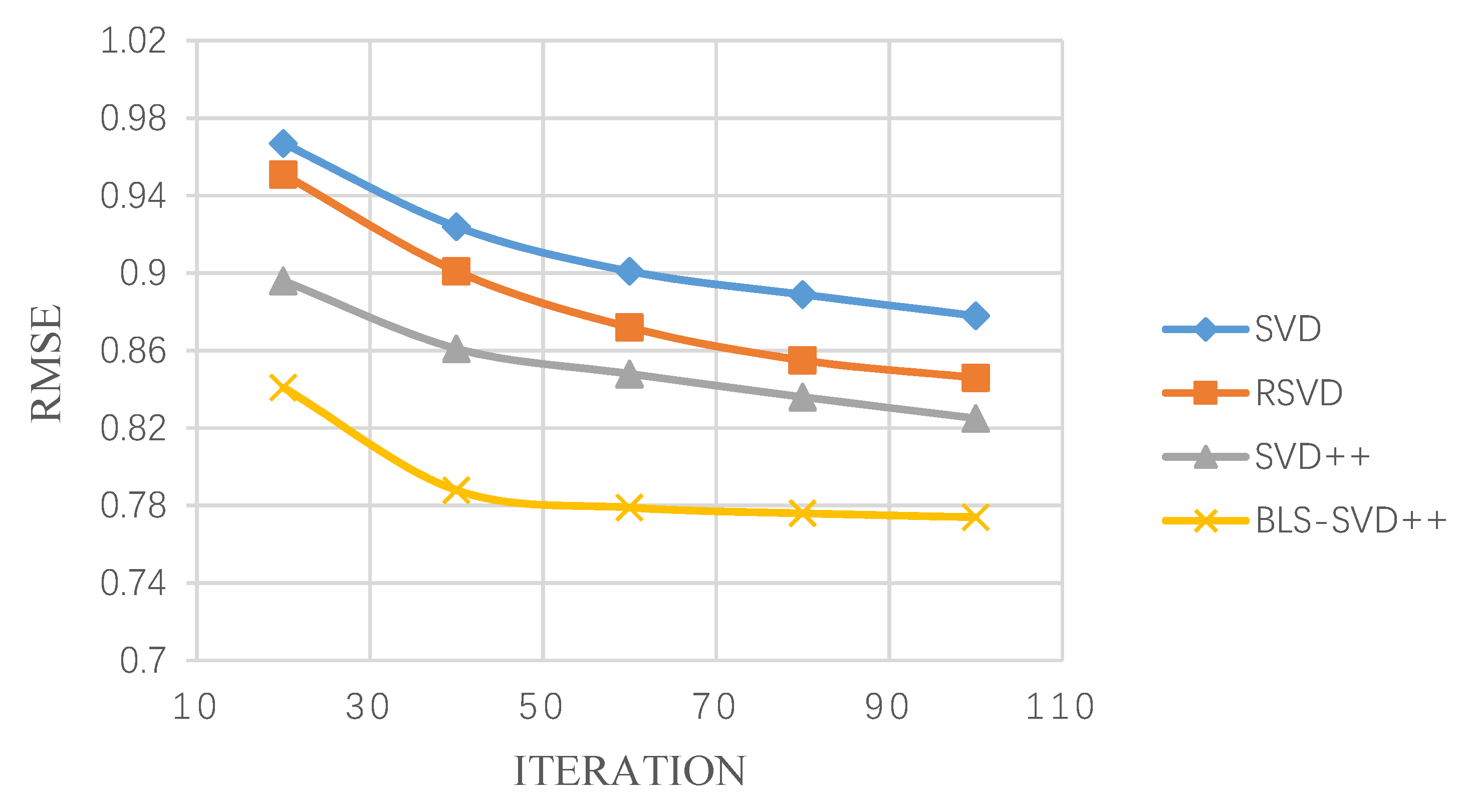
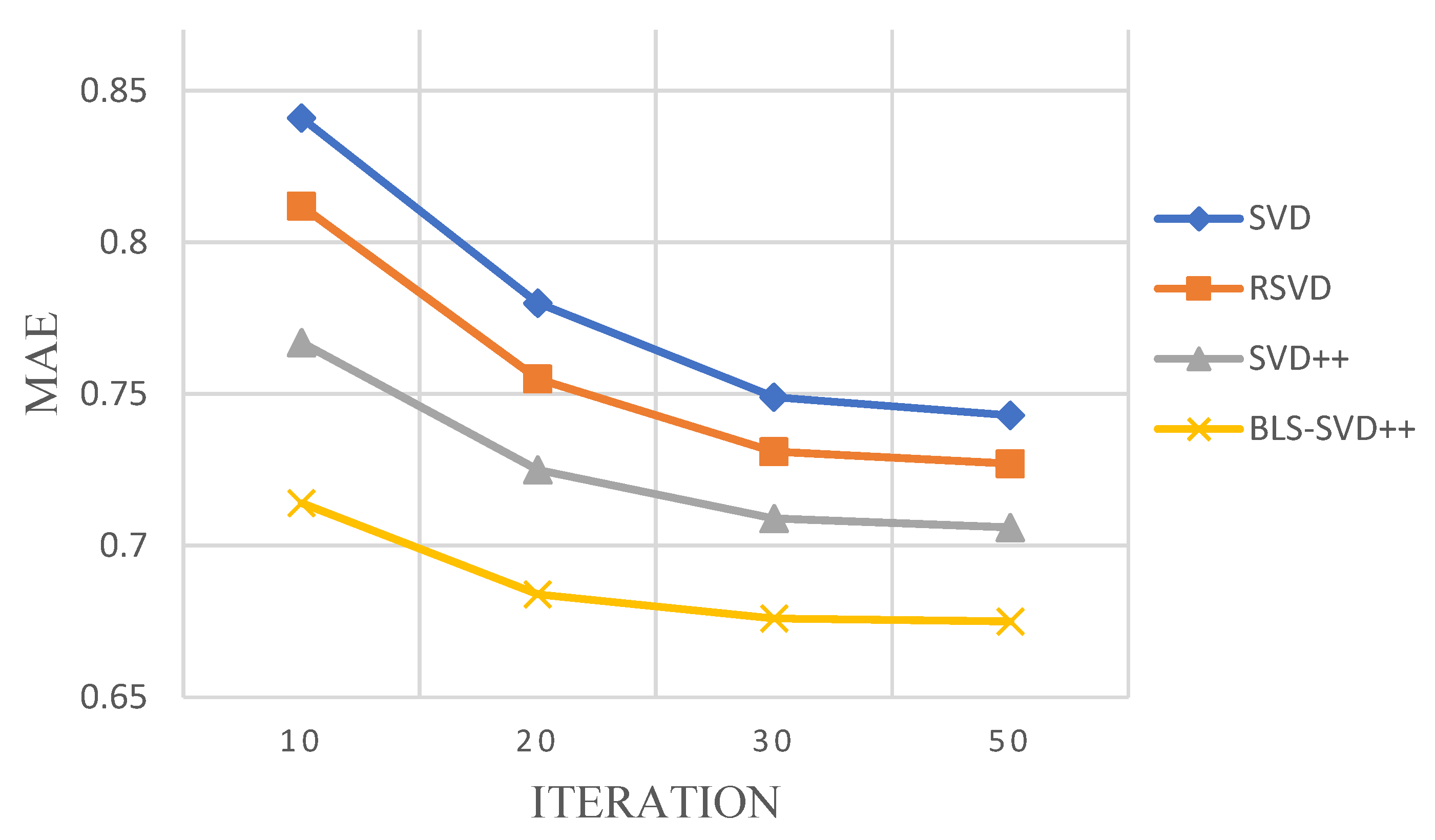
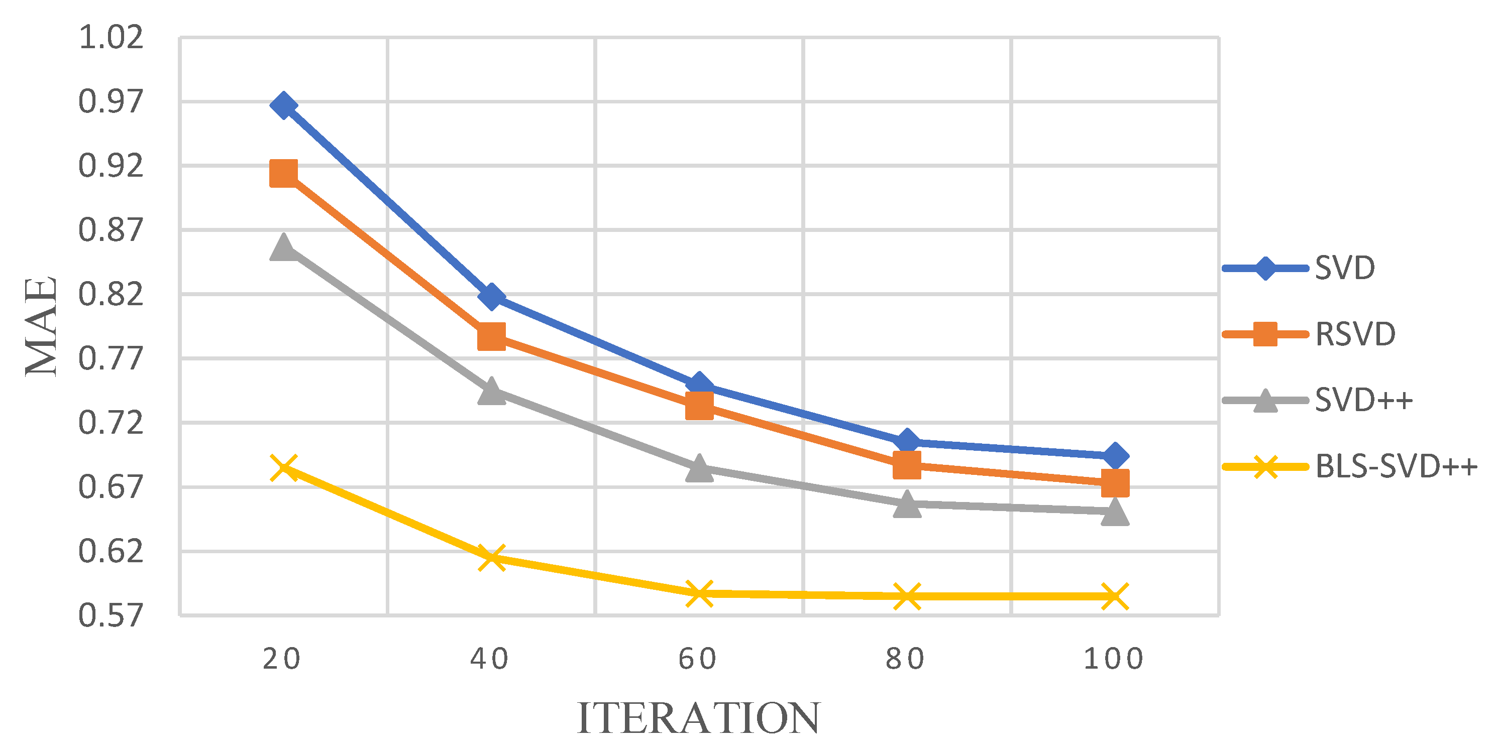
The BLS-SVD++ algorithm is compared with the conventional SVD++ and CF algorithms for MAE, RMSE and Recall experiments. The pairs under the RMSE and MAE evaluation criteria are shown in

Table 1. Comparison of RMSE results.

Dataset	RMSE
	SVD	RSVD	SVD++	BLS-SVD++
MovieLens 1 M	0.891	0.874	0.831	0.763
MovieLens 10 M	0.864	0.845	0.822	0.734
FilmTrust	0.903	0.887	0.853	0.826

and

Table 2. Comparison of MAE results.

Dataset	MAE
	SVD	RSVD	SVD++	BLS-SVD++
MovieLens 1 M	0.736	0.724	0.706	0.675
MovieLens 10 M	0.694	0.673	0.651	0.585
FilmTrust	0.790	0.758	0.725	0.707

. The RMSE changes with the number of iterations on the FilmTrust, MovieLens 1 M and 10 M data sets are presented in Figure 2, Figure 3 and Figure 4.

It can be seen from Table 1 and Table 2 that, compared with SVD, RSVD and SVD++, BLS-SVD++ has smaller RMSE and MAE values, indicating that the accuracy is higher than other recommended algorithms, and the prediction effect is better. Figure 2, Figure 3, Figure 4, Figure 5 and Figure 6 suggest that the BLS-SVD++ algorithm has a faster gradient degradation, and the number of iterations and time required to reach the optimal solution in the training is less than that of SVD++ and other recommended algorithms. In the experiment, by debugging different parameters, the resulting BLS-SVD++ algorithm achieves a four-fold reduction in the number of iterations than the SVD++ algorithm, and the recommended results are more accurate.

Moreover, on the platform built with the identical equipment. The single iteration time of the BLS-SVD++ algorithm reaches only 4–7% longer than that of the SVD++ algorithm. Since the device is not the latest computer, it is expected that, after the latest workstation is running, the time of each iteration of the BLS-SVD++ algorithm is only 1–3% longer than the original algorithm.

Via the analysis in Section 3 and experimental results, although the BLS-SVD++ algorithm slightly increases the time of a single iteration, the total number of iterations when the loss function reaches the optimal solution is greatly reduced. The total operation time of the algorithm when it reaches the optimal solution is reduced, which improves the overall efficiency of the algorithm.

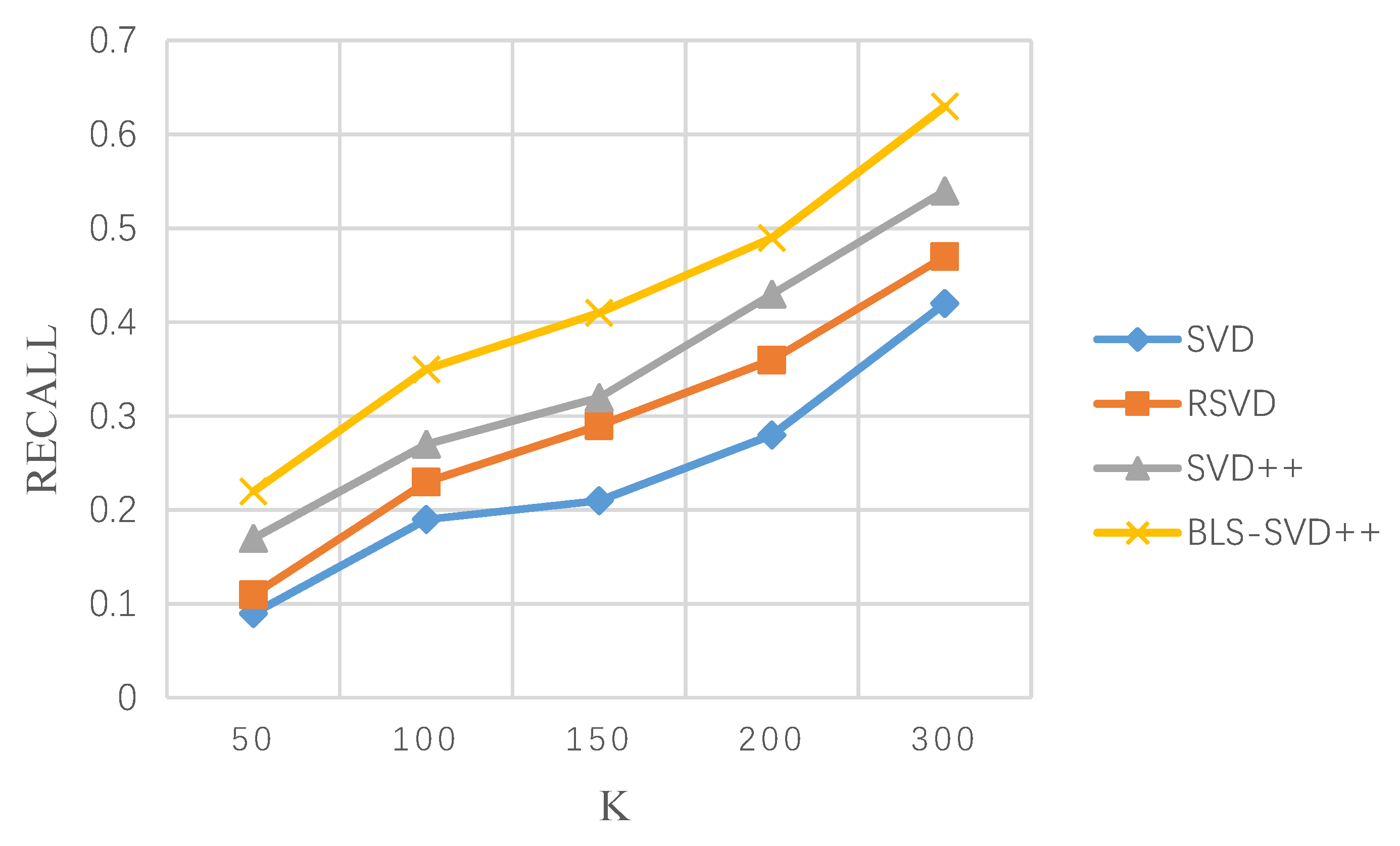
In the TOP-K recommendation, the recommended list length K is tested at different values, and the experimental results of K, 50, 100, 150, 200 and 300 are taken as samples and the recall rate is analyzed at MovieLens 1 M. The experimental results with the 10 M data set are listed in

Table 3. Comparison of Recall results in MovieLens 1 M database.

Module	Recommended List Length K
	50	100	150	200	300
SVD	0.09	0.18	0.21	0.28	0.42
RSVD	0.11	0.23	0.29	0.36	0.47
SVD++	0.17	0.27	0.32	0.43	0.54
BLS-SVD++	0.23	0.35	0.41	0.49	0.63

and

Table 4. Comparison of Recall results in MovieLens 10 M database.

Module	Recommended List Length K
	50	100	150	200	300
SVD	0.07	0.16	0.19	0.24	0.37
RSVD	0.09	0.20	0.23	0.32	0.41
SVD++	0.13	0.27	0.31	0.36	0.46
BLS-SVD++	0.16	0.32	0.38	0.45	0.55

below.

Figure 7 and Figure 8 suggest that the BLS-SVD++ algorithm is significantly optimized in the recall rate compared with the recommended algorithms (e.g., SVD++). In this study, the growth rate of the recall rate is larger than that of the comparison algorithm, demonstrating that the BLS-SVD++ algorithm achieves a high recall rate. The recommended item is capable of covering the entire user group with a higher ratio, and the recommended effect is more significant.

In brief, the BLS-SVD++ algorithm, based on backtracking line search in this study exhibits higher efficiency than the recommended algorithms (e.g., SVD and SVD++), and the number of iterations is lower in the training. The RMSE and MAE values are determined. Both are significantly reduced, and the accuracy of the achieved results is enhanced. For recall rate, the BLS-SVD++ algorithm is also significantly enhanced compared with other recommended algorithms. In the recommendation system, more accurate recommendation items are presented to users.

5. Conclusions

To increase the efficiency of SVD++ algorithm in the recommendation this study proposes to conduct a backtracking linear search in SVD++ algorithm, optimize the recommendation algorithm, and find the optimal solution based on the backtracking line search on the local gradient of the objective function.

By adding the judgment condition in the SVD++ algorithm, the learning rate of the algorithm is adaptive during the gradient descent process. In the primary stage, gradient descent is carried out at a relatively large learning rate and, in the middle and later stages, a smaller learning rate is used to search for the optimal solution. As revealed from the experiments on FilmTrust, MovieLens 1 M and 10 M datasets, the proposed BLS-SVD++ algorithm outperforms SVD and other recommended algorithms on RMSE and MAE. Moreover, Recall is compared on MovieLens 1 M and 10 M datasets. The experimental results prove that the BLS-SVD++ algorithm can reduce the overall calculation time by reducing the total number of iterations. Under the calculation efficiency, through the adaptive learning rate to search for the optimal solution, the final prediction result is more accurate.

Despite the good rating prediction effect, there are still some areas we ignored in this method. In future work, we will consider the introduction of new metrics to measure the proposed approach more comprehensively. We will continue to achieve more accurate and comprehensive predictions based on web page views, browsing stay time, social networks, and evaluation information.

References

- Wei, J.; Meng, F.; Arunkumar, N. A personalized authoritative user-based recommendation for social tagging. Future Gener. Comput. Syst. 2018, 86, 355–361. [Google Scholar] [CrossRef]
- Kluver, D.; Ekstrand, M.D.; Konstan, J.A. Rating-based collaborative filtering: Algorithms and evaluation. In Social Information Access; Springer: Cham, Switzerland, 2018; pp. 344–390. [Google Scholar]
- Yuan, X.; Han, L.; Qian, S.; Xu, G.; Yan, H. Singular value decomposition based recommendation using imputed data. Knowl. Based Syst. 2019, 163, 485–494. [Google Scholar] [CrossRef]
- Hu, J.; Liang, J.; Kuang, Y. A user similarity-based Top-N recommendation approach for mobile in-application advertising. Expert Syst. Appl. 2018, 111, 51–60. [Google Scholar] [CrossRef]
- Sahoo, A.K.; Pradhan, C.; Mishra, B.S.P. SVD based Privacy Preserving Recommendation Model using Optimized Hybrid Item-based Collaborative Filtering. In Proceedings of the 2019 International Conference on Communication and Signal Processing (ICCSP), Chennai, India, 4–6 April 2019; IEEE: Piscataway, NJ, USA, 2019. [Google Scholar]
- Tsaku, N.Z.; Kosaraju, S. Boosting Recommendation Systems through an Offline Machine Learning Evaluation Approach. In Proceedings of the 2019 ACM Southeast Conference, Kennesaw, GA, USA, 18–20 April 2019; pp. 182–185. [Google Scholar]
- Yin, Y.; Zhang, W.; Xu, Y.; Zhang, H.; Mai, Z.; Yu, L. QoS Prediction for Mobile Edge Service Recommendation with Auto-Encoder. IEEE Access 2019, 7, 62312–62324. [Google Scholar] [CrossRef]
- Liu, Y.; Zhong, X.; Li, L.; Yan, J. A Novel Algorithm for Group Recommendation Based on Combination of Recessive Characteristics. In Proceedings of the 2018 5th International Conference on Behavioral, Economic, and Socio-Cultural Computing (BESC), Taiwan, 12–14 November 2018; IEEE: Piscataway, NJ, USA, 2018. [Google Scholar]
- Royer, C.W.; Wright, S.J. Complexity analysis of second-order line-search algorithms for smooth nonconvex optimization. SIAM J. Optim. 2018, 28, 1448–1477. [Google Scholar] [CrossRef] [Green Version]
- Paquette, C.; Scheinberg, K. A stochastic line search method with convergence rate analysis. arXiv 2018, arXiv:1807.07994. [Google Scholar]
- Huang, W.; Absil, P.-A.; Gallivan, K.A. A Riemannian BFGS method without differentiated retraction for nonconvex optimization problems. SIAM J. Optim. 2018, 28, 470–495. [Google Scholar] [CrossRef] [Green Version]
- Wang, S.; Lo, D.; Vasilescu, B.; Serebrenik, A. EnTagRec++: An enhanced tag recommendation system for software information sites. Empir. Softw. Eng. 2018, 23, 800–832. [Google Scholar] [CrossRef] [Green Version]
- Manogaran, G.; Varatharajan, R.; Priyan, M.K. Hybrid recommendation system for heart disease diagnosis based on multiple kernel learning with adaptive neuro-fuzzy inference system. Multimed. Tools Appl. 2018, 77, 4379–4399. [Google Scholar] [CrossRef]
- Rebentrost, P.; Steffens, A.; Marvian, I.; Lloyd, S. Quantum singular-value decomposition of nonsparse low-rank matrices. Phys. Rev. A 2018, 97, 012327. [Google Scholar] [CrossRef] [Green Version]
- Raghuwanshi, S.K.; Pateriya, R.K. Accelerated Singular Value Decomposition (ASVD) using momentum based Gradient Descent Optimization. J. King Saud Univ. Comput. Inf. Sci. 2018. [Google Scholar] [CrossRef]
- Diniz, P.S.R. The least-mean-square (LMS) algorithm. In Adaptive Filtering; Springer: Cham, Switzerland, 2020; pp. 61–102. [Google Scholar]
- Jilg, A.; Bechstein, P.; Saade, A.; Dick, M.; Li, T.X.; Tosini, G.; Rami, A.; Zemmar, A.; Stehle, J.H. Melatonin modulates daytime-dependent synaptic plasticity and learning efficiency. J. Pineal Res. 2019, 66, e12553. [Google Scholar] [CrossRef] [PubMed]
- Medvedeva, M.A.; Simos, T.E.; Tsitouras, C. Variable step-size implementation of sixth-order Numerov-type methods. Math. Methods Appl. Sci. 2020, 43, 1204–1215. [Google Scholar] [CrossRef]
- Harrag, A.; Messalti, S. Ic-based variable step size neuro-fuzzy mppt improving pv system performances. Energy Procedia 2019, 157, 362–374. [Google Scholar] [CrossRef]
- Wang, W.; Lu, Y. Analysis of the Mean Absolute Error (MAE) and the Root Mean Square Error (RMSE) in Assessing Rounding Model. In Proceedings of the IOP Conference Series: Materials Science and Engineering, Kazimierz Dolny, Poland, 21–23 November 2019; IOP Publishing: Bristol, UK, 2018; Volume 324, p. 012049. [Google Scholar]
- Vann, J.C.J.; Jacobson, R.M.; Coyne-Beasley, T.; Asafu-Adjei, J.K.; Szilagyi, P.G. Patient reminder and recall interventions to improve immunization rates. Cochrane Database Syst. Rev. 2018, 1, CD003941. [Google Scholar]
- Portugal, I.; Alencar, P.; Cowan, D. The use of machine learning algorithms in recommender systems: A systematic review. Expert Syst. Appl. 2018, 97, 205–227. [Google Scholar] [CrossRef] [Green Version]
Figure 1.
Scoring Matrix.
Figure 2.
FilmTrust dataset RMSE varies with iterations.
Figure 3.
MovieLens 1 M dataset RMSE varies with iterations.
Figure 4.
MovieLens 10 M dataset RMSE varies with iterations.
Figure 5.
MovieLens 1 M dataset MAE varies with iterations.
Figure 6.
Figure 7.
MovieLens 1 M dataset recall rate varies with recommended list length K.
Figure 8.
MovieLens 10 M dataset recall rate varies with recommended list length K.