Mobile Money Fraud Prediction—A Cross-Case Analysis on the Efficiency of Support Vector Machines, Gradient Boosted Decision Trees, and Naïve Bayes Algorithms

Abstract

The onset of COVID-19 has re-emphasized the importance of FinTech especially in developing countries as the major powers of the world are already enjoying the advantages that come with the adoption of FinTech. Handling of physical cash has been established as a means of transmitting the novel corona virus. Again, research has established that, been unbanked raises the potential of sinking one into abject poverty. Over the years, developing countries have been piloting the various forms of FinTech, but the very one that has come to stay is the Mobile Money Transactions (MMT). As mobile money transactions attempt to gain a foothold, it faces several problems, the most important of them is mobile money fraud. This paper seeks to provide a solution to this problem by looking at machine learning algorithms based on support vector machines (kernel-based), gradient boosted decision tree (tree-based) and Naïve Bayes (probabilistic based) algorithms, taking into consideration the imbalanced nature of the dataset. Our experiments showed that the use of gradient boosted decision tree holds a great potential in combating the problem of mobile money fraud as it was able to produce near perfect results.

1. Introduction

Connectivity through telecommunications has remodeled our way of lives. The use of mobile handsets have had a tremendous impact on our very existence. In most developed countries and some emerging economies, one can do anything from having a virtual medical appointment with a doctor, undertaking all forms of commerce and virtually everything that one can imagine through the use of mobile handsets. One important innovation brought about by mobile handsets is the ability to perform financial transactions using mobile devices. For example, in China, WeChat and Alipay are important applications that can be used to undertake quite a number of financial transactions [1,2], with advanced inbuilt security features using smartphones. These advances through the use of mobile phones enjoyed in these developed countries are virtually non-existent in most developing countries. In most developing economies, predominantly in sub-Saharan Africa, undertaking financial transactions with both feature phones and smartphones through the use of short message services (SMS) and other mobile applications has been on the ascendency. This is popularly known as mobile money transactions (MMTs) and has questionable security features. These loopholes in security and lack of education (anecdotally) on the part of users of have created space for criminals to engage in fraudulent activities making customers lose a lot of fortune and impeding the prospect of rolling the unbanked into the FinTech community. Research in the field of providing security for MMTs have been very minimal partly due to the fact that these forms of electronic transactions are virtually unknown to the developed world. Detecting frauds in mobile money has been a colossal task. Stakeholders have used rule and other statistically-based methods in an attempt to detect and prevent fraudulent transactions. These methods have, however, failed woefully as there are incessant reports from many dailies in the developing world with news of one form of mobile money fraud and has become a key topic of research [3,4,5,6]. This has a high potential of rolling back the huge inroads made by MMTs. Machine and deep learning methods are emerging fields that have been employed extensively in the field of finance to detect and prevent fraud [7,8]. These machine and deep learning methods, have shown potential improvements in combating financial fraud [9,10].

This article investigates the performance of three machine learning classifiers chosen from Support vector machines (SVM) (kernel-based), Gradient Boosting Decision Tree (tree-based) and Naïve Bayes (probabilistic classifiers). With a mind on the highly imbalanced nature of data from financial transactions such as the dataset used in this article, we explored further by performing different sampling methods before using the dataset to train our ML algorithms for classification and prediction. The organization of the rest of the work is as follows. In Section 2, we undertake a review of current related literature. Section 3 presents the Mobile Money (MM) ecosystem. Section 4 provides an introduction to Machine Learning (ML), describes the mathematical and theoretical backgrounds of our selected machine learning algorithms. Section 5 describes the dataset, experimental setup and methods. Section 6 presents our performance evaluation metrics. In Section 7, we present and discuss the results from our experiment and conclude our article in Section 8.

2. Related Work

Literature related to Fraud prevention with machine learning, data imbalance and Fraud prevention were reviewed. With a daily increase in fraud across the financial sector [11], various methods have been and continues to be explored on ways to combat such ills [12]. Traditionally, financial institutions have used rule and statistically based systems for fraud prevention [13]. Machine and deep learning algorithms are now increasingly been used in detecting and preventing fraud in this all-important arena. Singh et al. [10] used SVM with multiple kernels to detect fraud in credit card transactions. Their experiment rated Radial Basis Function (RBF) as the best kernel in comparison with linear and the quadratic kernels. The paper, however, failed to discuss the inherent nature of imbalance data related to credit card transactions. Reference [14] worked on credit card fraud detection with deep learning based on auto-encoder and restricted Boltzmann machine. The authors argued for their method based on the fact that most supervised learning algorithms work by using behavioral patterns of “legitimate” user’s spending behavior to detect abnormalities as fraud, bearing in mind also that the “legitimate” user’s behavior can change thereby causing the algorithm to wrongfully classify legitimate transactions as illegitimate. They, therefore, called for the use of unsupervised machine learning algorithms hence their approach. Randhawa et al. [15] experimented both standard models and hybrid methods making use of AdaBoost and majority voting. They, again, introduced noise to the dataset to evaluate the robustness of their model. They concluded on majority voting as achieving a very good accuracy in detecting fraud in credit cards. Tran et al. [16] focused their work on real-time data-driven approaches for detecting fraud in credit cards. The paper introduced two (2) real-time data-driven approaches using optimal anomaly detection techniques with data from European credit card holders and concluded that their experiments achieved a high-level of detection and a low percentage of false alarms. In their paper “Credit card fraud detection based on Whale algorithm optimized BP neural network” [17], the authors aimed at solving the problem of slow convergence rate by looking at the Whale Swarm Optimization Algorithm (WOA). They first used WOA to obtain an initial optimal value then used BP network algorithm to correct the error value to obtain the optimal value. Akila et al. [18] used cost-sensitive Risk Induced Bayesian Inference Bagging to detect fraud in credit cards. They experimented their method on Brazilian bank data and reported 1.04–1.5 times reduction in cost. The robustness of their model was also reported by performing experiments on UCSD-FICO data. Their model was also reported to handle unseen data without the need for any domain-specific parameter fine-tuning. Husejinović [19] experimented with naive Bayesian and C4.5 decision tree classifiers in an attempt to prevent fraud in credit card transactions. The performance of the experiments was evaluated through precision, recall, and PRC area rates. The researcher concluded by reporting a success rate of 92.74% using C4.5 decision tree algorithm. Adeyinka et al. [20] provided a great insight into predicting fraud in mobile money transfer. Their work was based on Case-Based Reasoning (CBR) which is an alternative to standard machine learning methods. Their method, however, made use of machine learning techniques such as k-Nearest Neighbor (k-NN) to assign parameter weights in the dataset. It also used genetic algorithm (GA) as a tool to optimize the significance level of (weights). The authors demonstrated that the classification of log information into five contexts and recombining them into a single dimension rather than the traditional approach which made use of amount, time, or feature dimensions as individual parameters improved the performance of their weighted CBR system with an accuracy of 0.97% and 0.98%. Fiore et al. [21] proposed the use of adversarial neural networks to detect fraud in credit card transactions. While their method resulted in improved results, neural networks, however require large datasets and are computationally expensive. Carcillo et al. [22] combined both supervised and unsupervised learning methods to predict fraud in credit card transactions but as with similar methods, data for unsupervised learning remains a problem. Other researchers have used other machine learning methods to detect and predict fraud in finance [23,24] but most failed to properly address the problem of data imbalance. Data imbalance—the problem of data imbalance remains a quagmire to data scientist as it can negatively alter the performance of machine and deep learning algorithms [25]. Several approaches for handling data imbalance have been proposed by various authors. Reference [26] proposed the use of undersampling and oversampling methods to deal with the problem of class imbalance. Other approaches such as synthetic minority oversampling technique (SMOTE) [27], adaptive synthetic (ADASYN), oversampling [28] and undersampling [29] have been proposed. Evaluation metrics. There are a variety of metrics to evaluate machine learning algorithms such as accuracy, precision, recall, F1 Measure, and so forth, where each metrics portrays a different set of information about the performance of the machine or deep learning model. Thus different evaluation metrics should be used for different scenarios so as adequately present the performance of an algorithm. Hossin and Sulaiman [30] in their article “a review on evaluation metrics for data classification evaluations,” vividly explained the role and importance of metrics. For example, using model accuracy as the only evaluation metric for a dataset such as those form MMTs will send a wrong signal about the model due to the imbalance nature of the dataset. From the review of the related literature, we performed experiments with different machine learning models based on SVM, Gradient Boosting Decision Tree and Naïve Bayes algorithms for classifying and predicting fraud in MMTs by first observing the effect of undersampling and oversampling and finally a combination of both.

3. The Mobile Money Ecosystem

The mobile money system started as M-Pesa in Kenya which was introduced by the telecommunication company Safaricom in 2007 [31]. There are three (3) key actors in the mobile money ecosystem. The user (mobile money account holder), the telecommunication company providing the service and the mobile money agents. Users accrue funds in their wallet either through direct deposits or by third parties (business partners, family, non-governmental organizations (NGOs), etc.). Deposits, withdrawals, and payments are initiated through peer-to-peer (P-2-P) accounts, mobile money agents, retail shops of the telecommunication companies, and recently, through some selected banks. A successful transaction is indicated by a short message service (SMS). The successful implementation of M-Pesa quickly spread to other countries in Africa and other developing economies. Today, there are over 1.2 billion people with mobile money accounts around the world making transactions worth two (2) billion United State Dollars in 2019. Sub-Saharan Africa accounted for around fifty (50) million new subscribers [32].

Table 1. Regional growth of Mobile Money in 2019.

	Registered Accounts	Active Accounts	Transaction Volume	Transaction Value (USD)
Global	1.04 Billion	372 Million	37.1 Billion	690.1 Billion
East Asia and Pacific	158 Million	60 Million	4.4 Billion	78.9 Billion
Europe and Central Asia	20 Million	7 Million	217 Million	3.8 Billion
Latin America and Caribbean	26 Million	13 Million	601 Million	16.5 Billion
Middle East and North Africa	51 Million	19 Million	663 Million	9.1 Billion
South Asia	315 Million	91 Million	7.3 Billion	125.4 Billion
Sub-Saharan Africa	469 Million	181 Million	23.8 Billion	456.3 Billion

represents the regional growth of mobile money transactions as reported by Reference [32] in 2019.

Table 2. Growth of Mobile Money in Sub-Saharan Africa for 2019.

	Registered Accounts	Active Accounts	Transaction Volume	Transaction Value (USD)
East Africa	249 Million	102 Million	17.1 Billion	293.4 Billion
Central Africa	48 Million	20 Million	1.8 Billion	30.4 Billion
South Africa	9 Million	3 Million	165 Million	2.5 Billion
West Africa	163 Million	56 Million	4.8 Billion	130.0 Billion

gives a further breakdown of Africa [32] and

Table 3. Growth of Mobile Money in Ghana.

	2016	2017	2018	January–March 2018	January–March 2019	2019 % Growth
Registered MM Accounts	19,735,098	23,947,437	32,554,346	25,306,085	29,578,169	16.88
Active MM Accounts	8,313,283	11,119,376	13,056,978	11,248,758	12,725,649	13.3
Registered Agents	136,769	194,688	396,599	217,974	355,912	63.28
Active Agents	107,415	151,745	180,664	161,317	182,344	13.03
Total Volume of Transactions	550,218,427	981,564,563	1,454,470,801	312,926,881	436,723,487	39.56
Total Transactions( Million)Cedis	78,508.90	155,844.84	223,207.23	52,352.80	66,356.41	26.75

presents the report on the growth of MMT in Ghana spanning 2016 to 2019 as reported by the Bank of Ghana [33].

3.1. The Case of the Unbanked in the Developing World

In Africa and other parts of the developing world, the number of unbanked is very large regarding the size of the population compared to the developed world. According to Reference [34] from the World Bank Group, account ownership is nearly universal in high-income economies, putting virtually all unbanked adults in developing economies. The reasons below are some of the contributing factors that account for this phenomenon.

• In the developing world, banking is considered a prerogative for the rich in society since they can afford the regular and expensive fees that come with regular banking.
• Banking is considered to be “something” for those in urban areas where banks are easily accessible [31]
• People tend to avoid the patronage of the traditional banking system due to overcrowding, slow access to services, and the continuous excuse of “network down” so we can not serve you.
• Banks are few which translates to the fact that people have to travel long distances on deplorable roads coupled with the additional risk of being attacked by thieves.
• Cumbersome account opening requirements [20].

3.2. Regulating MMTs, the Role of Central Banks and Telecommunication Companies

The central bank of every country plays a crucial role in the regulation of all financial activities carried out in the country. MMT which involves monetary transactions falls under the regulation of the central bank. Telecommunication companies enforce the regulations and frameworks that are developed and set up by the central bank and other authorities like the national communications authority (NCA) in Ghana that regulate all activities related to spectrum management. According to the Global System for Mobile Communications (GSMA) [32], regulations that enable low-cost services for the financially excluded has been crucial to the success of mobile money. There is, therefore, a clear correlation between countries with high mobile money adoption rates and more enabling regulatory environments. In India for example, a lot of payment banks surrendered their licenses to the Reserve Bank of India citing increasingly burdensome regulatory and operating environments [32]. The reverse has been the case in most other places especially in sub-Saharan Africa. Per the Bank of Ghana’s two key objectives of the payment system in Ghana, it wants to:

• Discourage the use of physical cash for transactions and
• Enable the integration of an electronic payment system

Looking at the objectives of the Central Bank, telecommunication companies that operate mobile money can only be seen as agents of development and not the opposite. However, some problems arise from this regulatory regime by Central Banks. Central Banks recognize these telecommunication companies as merely providing telecommunication infrastructure for payment system [20] thereby playing only passive roles. Works are ongoing for proposals to develop a legislative framework to properly streamline the operations of MMTs. The GSMA which represents the interest of mobile operators worldwide has instituted the Mobile Money Regulation Index (MMRI) which is a regulatory tool that provides a quantitative assessment of the extent to which regulation has been effective in establishing enabling regulatory environments. Due to the rapidly changing nature of MMTs such as the payment of remittances from relations abroad and others such as MMTs operating as insurance providers, regulatory bodies need to constantly adjust existing frameworks and policies to make up for the rapidly changing landscape as cumbersome regulations prevent innovations in MMTs. To protect the vulnerable, in the era of COVID-19, governments and some MMT providers and their regulators have responded with several measures aimed at achieving two broad outcomes:

• Limiting the spread of the COVID-19 virus by encouraging digital payments
• Easing the burden of the living cost on people who use digital payments through the following measures such as

• Waiving P-2-P transaction fees
• Support for mobile money agents
• Waiving interchange fees.

4. Machine Learning Algorithms

This section gives an introduction to Machine Learning, describes the machine learning algorithms used in this paper as well as the mathematical foundations that establish them. Machine learning is a branch of Computer Science that deals with making computers learn to imitate humans by feeding the computer with data and information while the computer is not explicitly programmed. It can be described as a nine step process which involves the following:

• Definition of an objective
• Collection of relevant data in line with the objective
• Preparing and preprocessing the data
• Selection of the relevant machine learning algorithm
• Training the selected ML algorithm with the preprocessed data from step 3
• Testing the trained ML algorithm in step 5 with the test data
• Testing the fitness of the model and adjusting where necessary
• Performing predictions or classifications with the model
• Deploying the model to solve real-world problems

ML can be grouped into three main types;

• Supervised
• Unsupervised
• Reinforced machine learning.

Supervised ML is the type of ML that normally performs predictions or classifications based on labeled data. Examples of supervised ML algorithms are SVM and Decision Trees. Unsupervised ML algorithms perform their task without the use of labeled data but can identify hidden patterns in the unlabeled dataset fed to it. Examples of unsupervised ML algorithms are Anomaly Detection and K-Means. Reinforced learning is a type of ML where an agent learns how to behave in an environment through the performance of actions and observing the results to make needed modifications. An example of reinforced learning is a computerized chess game. This work made use of supervised ML algorithms, namely, SVM, DT, and NB. Our chosen algorithms are discussed in the sections below.

4.1. Support Vector Machines

Support vector machines (SVM) is a supervised machine learning algorithm for solving regression and classification problems with the latter been used predominantly. It has the capability of detecting complex hidden patterns. The robustness of SVM and its ability to integrate with kernel-based learning makes SVMs a more flexible analysis and optimized solution for classification problems [26]. For two dimensional data, SVM works by trying to divide the two classes of data by a hyperplane the splits the classes in the best possible way. This maximizes the distance between the nearest points (support vectors) to the hyperplane on both classes thereby maximizing the margin between the support vectors on both sides. This is illustrated in Figure 1. This becomes a constrained optimization problem which can be solved using Lagrange multipliers.

For a linearly separable data, a number of feature vectors z are given as inputs,

$$\begin{array}{c}\hfill M=(x_z,y_z)\end{array}$$

(1)

Such that $x_z$ and $y_z\in {\mathbb{R}}^d$ to output an instance class $y_i$ using the parameters w and b. The classification decision is made as follows:

$${\mathrm{y}}_{\mathrm{i}}=\left\{\begin{array}{cc}\hfill 0,& w^{M}x+b=0\hfill \\ \hfill -1,& w^{M}x+b\le -1\hfill \\ \hfill 1,& w^{M}x+b\ge 1\hfill \end{array}\right.$$

(2)

where

$$y_i=\{1,-1\}$$

(3)

are the instance classes of frauds whilst

$$y_i=0$$

(4)

represents the hyperplane used for the classification.To maximize the distance (margin) between the support vectors on sides of the classes, we minimize

$$\frac{1}{2}{\parallel w\parallel }^2+C\sum _{i=1}^Z{\xi }_i$$

(5)

Subject to the linear inequality constraints

$$y_i\left(w^M{x}_i+b\right)\ge 1-{\xi }_i,{\xi }_i\ge 0,i=1,\dots ,z$$

(6)

where ${\xi }_i$ is the slack variable that allows for misclassifications to occur and C is the regularization parameter that controls the tradeoff between the margin and the misclassification error. From Equation (5), dual formulation will be used to solve the minimization problem as,

$$min\frac{1}{2}\sum _{i,j}^M{y}_i{y}_j{\alpha }_i{\alpha }_{j}k\left(x_i,x_j\right)-\sum _{i=1}^M{\alpha }_i$$

(7)

For our dataset having $d>2$, which is non-linearly separable, our data was mapped into a higher dimensional space using the kernel trick. This work relied on GridSearchCV from sklearn to search for the best kernel and other hyperparameters for our SVM algorithm to best fit our data at hand. Polynomial, Radial Basis Function (RBF) and the sigmoid kernels were utilized.

4.2. Decision Tree

Decision Tree is a class of supervised learning algorithms that can be used for the purpose of both classification and regression. It takes the form of a tree that is used to determine the course of action. Decision trees provide a graphical representation of all the possible solutions. Decisions are based on certain conditions where each branch of a tree represents a possible solution. A tree has a root node representing the topmost decision as well as the highest entropy without any incoming edges whereas the other nodes have only one incoming edge know as decision node. The leaf nodes are the class labels and carries the classification or the decision and the attributes are the internal nodes. To classify a given set of data using decision trees, conditions have to be framed such that either the information gain is the highest or the Gini index is the lowest [35]. Thus the attribute selection process is based either on the information gain or the Gini index.

4.3. Entropy

Entropy is defined as the measure of randomness or unpredictability in the dataset. Given a number of k classes, the information gain is given mathematically by [35]

$$\sum _{i=1}^{k}P\left(i\right)\ast {log}_2\left(P\left(i\right)\right)$$

(8)

, where $P\left(i\right)$, is the percentage of the class in a node.

4.4. Information Gain

Information gain is the measure of decrease in entropy after splitting the dataset. It is one of the selection criteria for decision trees. In this method, the condition that gives the highest information gain is to be selected for the splitting process [36,37]. The entropy is calculated after each split. The information gain is then calculated as the difference between the entropy values after the split. This process of splitting the dataset is a recursive one and only terminates when the value of the entropy reaches 0. It starts with a root node and then branches off to any number of solutions.

4.5. Gini Index

The Gini index is a metric used to measure the frequency at which a randomly chosen elements would be wrongly classified. We always aim for a lower Gini index. It is given by;

$$GI=1-\sum j{P}_j^2$$

(9)

where $P_j$, is the percentage of a the class in a node [37].

4.6. Gradient Boosted Decision Tree

Decision tree belongs to a group of machine learning algorithms that are considered weak learners. In order to increase the accuracy of our decision tree model, we employed gradient boosting which is an ensemble learning technique with the capability of increasing the accuracy of our weak learner; decision tree into a strong learner by sequentially generating the decision tree in such a way that present one is always better than the previous. This is achieved by adding a new adaptive model to optimize the loss function of the previous decision tree algorithm [38,39,40]. GridSearchCV was employed to obtain the optimized hyperparameters in this paper.

4.7. Naïve Bayes

Naïve Bayes is a supervised machine learning algorithm for both classification and regression that works on the concept of naïvetés (independence of attributes) and on the principle of conditional probability defined by Bayes’ theorem. The Bayes’ theorem gives the conditional probability of an event A given that event B has occurred [37,41]. It can be represented mathematically as

$$\mathrm{P}(\mathrm{A}\mid \mathrm{B})=\frac{\mathrm{P}(\mathrm{B}\mid \mathrm{A})\mathrm{P}\left(\mathrm{A}\right)}{\mathrm{P}\left(\mathrm{B}\right)}$$

(10)

$P(A÷B)$ is the posterior probability, $P(B÷A)$ is the likelihood, $P\left(A\right)$ is the prior probability, and $P\left(B\right)$ is the evidence [42]. Applying this concept to the machine learning classification problem, if $B_1,B_2,\dots ,B_n$ are the features of a labeled data, then to predict a target A, given the features B, we can write

$$\mathrm{P}\left(\mathrm{A}\mid {\mathrm{B}}_1,{\mathrm{B}}_2,\dots ,{\mathrm{B}}_{\mathrm{n}}\right)=\frac{\mathrm{P}\left({\mathrm{B}}_1,{\mathrm{B}}_2,\dots ,{\mathrm{B}}_{\mathrm{n}}\mid \mathrm{A}\right)\mathrm{P}\left(\mathrm{A}\right)}{\mathrm{P}\left({\mathrm{B}}_1,{\mathrm{B}}_2,\dots ,{\mathrm{B}}_{\mathrm{n}}\right)}$$

(11)

.

Then for n features with the class label Y, it can be written as

$$\mathrm{P}\left({\mathrm{X}}_1,{\mathrm{X}}_2,\dots ,{\mathrm{X}}_{\mathrm{N}}\mid \mathrm{Y}\right)=\prod _{\mathrm{i}=1}^{\mathrm{n}}\mathrm{P}\left({\mathrm{X}}_{\mathrm{i}}\mid \mathrm{Y}\right)$$

(12)

where P(Y) becomes the class probability and $P\left(X_i\mid Y\right)$ the conditional probability.

Naïve Bayes (NB) is considered to be one of the very fast algorithms used for classification purposes and a good one for handling large volumes of data. The NB algorithm operates on the principle that the features or variables in a dataset are unrelated. There are 3 main variants of the NB algorithm; Gaussian(GS), Multinomial(MN), and Bernoulli(BN). Gaussian is used when the features or characteristics values are continuous and the assumption made that the value linked with each class is dispersed based on the Gaussian distribution that is to say normal distribution. Multinomial is used for instances where there is a multinomial distribution of data and specialized for text documents. Bernoulli is used when data is dispersed according to Multivariate Bernoulli distribution. This paper, experimented all three types of the NB algorithms to determine which one best suits our dataset at hand.

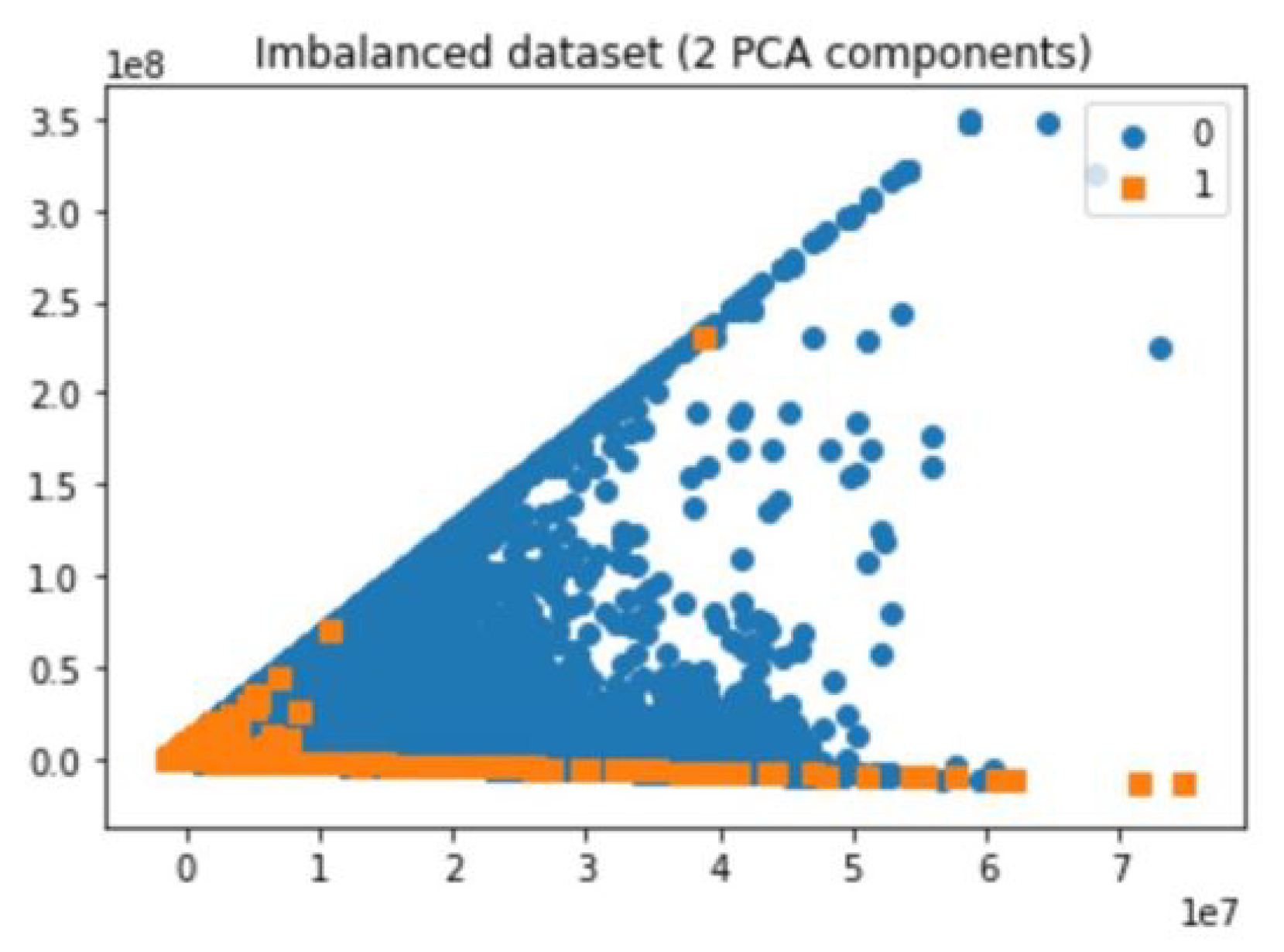
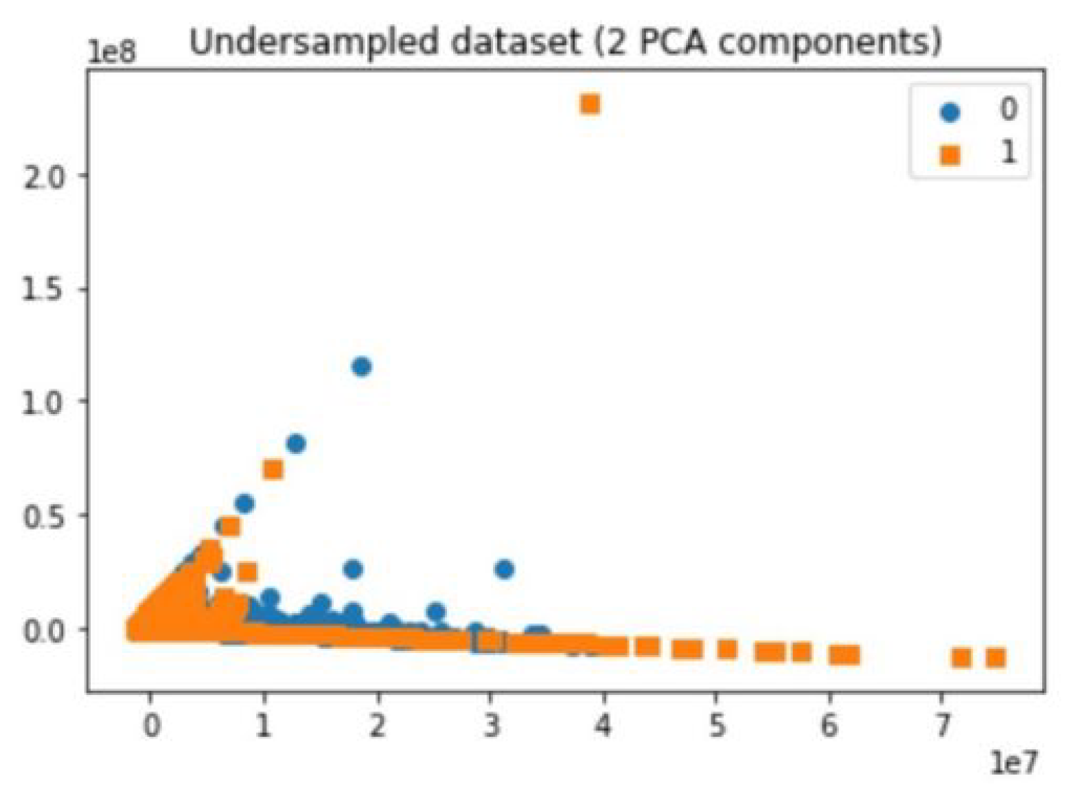
5. The Dataset, Experimental Setup and Methods

This section describes dataset, and the process and methods involved in obtaining our results. The experiments were carried out on a computer running Microsoft Windows Server 12 edition with Intel(R) Xeon(R)CPU E5-2640 v3 @ 2.60 GHz and 191.87 GB of RAM.

5.1. The Dataset

The dataset for this experiment was sourced from Kaggle. The dataset was generated from transactional logs from a mobile money service provider in an African country whose operations span over 14 countries around the world [43]. The dataset consists of nine attributes and a target with descriptions as follows:

• type—CASH-IN, CASH-OUT, DEBIT, PAYMENT, and TRANSFER, which are the main types of transactions under MMT.
• amount—amount of the transaction in local currency.
• nameOrig—customer who started the transaction
• oldbalanceOrg—initial balance before the transaction
• newbalanceOrig—new balance after the transaction
• nameDest—customer who is the recipient of the transaction
• oldbalanceDest—initial balance recipient before the transaction
• newbalanceDest—new balance recipient after the transaction.
• isFraud—This is the transaction made by the fraudulent.
• isFlaggedFraud—The business model aims to control massive transfers from one account to another and flags illegal attempts. An illegal attempt in this dataset is an attempt to transfer more than 200,000 in a single transaction.

5.2. Model Construction

Analysis performed on the dataset revealed that the feature “type” contained string data which was subsequently converted to numeric using one-hot encoding. The dataset, paysim1 was explored further visually using seaborn plot and its various features examined using chi-squared $\left(ch{i}^2\right)$ score. Also, features whose p values were determined to be greater than $0.5$ were eliminated since they will not have any significant effect on the model. From the results, we selected the five best features, Transfer, newbalanceOrig, oldbalanceDest, amount, and oldbalanceOrg for the construction of the model since the rest of the features showed no significant contribution.

In order to prevent the curse of data imbalance, the data were explored to see the distribution before proceeding with the model development. The dataset consist of a negative class (0) made up of 99.8709% and positive class (1) made up of 0.1290%. A 2 Principal component analysis (PCA) representation of the dataset is presented in Figure 2. This shows a very high level of data imbalance in the dataset and any model developed with this dataset without any sampling technique will be biased towards the negative class. In this paper, a model with the original dataset was first developed without performing any sampling on the dataset. Two (2) undersampling procedures namely NearMiss and RandomUnderSampling, two (2) oversampling procedures RandomOverSampler and SMOTE, and a combination of both for the classifiers SVM and NB were performed. That is, five (5) experiments were performed for SVM and fifteen (15) for NB; five (5) for GS, BN, and MN. DT however, can handle the problem of class imbalance so the experiment was performed on GBDT using the original dataset without any sampling but was carried out with optimized hyperparameters.

5.3. Undersampling

Undersampling is the process of reducing the size of the majority class in a dataset in an attempt to make even the sizes of both the majority and the minority class. This helps in making sure that ML models created from the dataset will not be biased towards the majority class. Undersampling, however, has a potential problem of removing a chunk of information from the dataset. For undersampling two different sampling methods; random undersampler and Near Miss were considered.

5.4. Random Undersampler

RandomUnderSampler from imblearn was used. This is a type of a prototype selection algorithms use the same reference such that given the original majority class as a set T, The new majority class (set, $T^{rus}$) obtained by the resampling process is such that $\left|T^{rus}\right|<\left|T\right|$ and $T^{rus}ϵT$ [44]. In this method, the majority class was uniformly and randomly undersampled. This process can also lead to the loss of important information from the dataset. In this article, the auto parameter from the model was used in an attempt to equalize the length of both the minority and majority classes. A scatter plot of the data after performing RandomUnderSampling using a 2 PCA representation for the data is presented in Figure 3.

5.5. NearMiss

Near miss is made of a number of different methods for reducing the size of the majority class which is based on distance of majority class examples to minority class examples [45]. It operates by removing randomly some of the majority samples in the dataset. It does so by removing instances of the majority class when two (2) different classes are very close to each other thereby increasing the space between the two classes to help in the classification process, and also reduce the size of the majority class.

5.6. Tomek Links

Tomek links is an undersampling technique for reducing the size of the majority class. Given two instances $x_i$ and $x_j$ where $x_i$ and $x_j$ belong to two different classes, (minority and majority respectively) then they are said to form a Tomek-link pair, if there is no sample $x_k$ such that $d\left(x_i,x_k\right)<d\left(x_i,x_j\right)$ [46]. The algorithms seek to clarify the boundary between the majority and the minority class, making the minority regions more distinct. From References [47,48], the algorithm can be used both as an undersampling technique or for post-process cleaning up. For undersampling, only samples from the majority class are removed. For post-process cleaning samples from both classes are removed. After oversampling, most often, the classes groups are not well defined, meaning samples from both classes may be invading each other. In this paper, the algorithm was used as a post-process cleaning step.

5.7. Oversampling

In oversampling, the idea is to increase the size of the minority class with synthetic data points for the minority class to match up to that of the majority class. This enables machine learning algorithms to develop models that are not biased to any of the classes since both classes have roughly the same number of samples for the model development phase. There are several types of oversampling algorithms such as adaptive synthetic sampling approach(ADASYN) and SMOTE. In this article, the authors considered SMOTE and RandomOverSampler.

5.8. Random Oversampler

Our oversampling approach utilized the RandomOverSampler from the imblearn library [49]. RandomOverSampler works by creating additional data points from the minority class to make up for the shortfall in its length. This enables the decision function of the classifier to make informed decisions as both classes are equally represented.Oversampling increases the weight of the minority class through a replication process. Whereas oversampling does not add any extra information to the dataset, it causes an increase in the likelihood of overfitting. A 2 PCA representation for the data after oversampling is presented in Figure 4.

5.9. Synthetic Minority Oversampling Technique (SMOTE)

SMOTE is an oversampling method that attempts to create synthetic data points for the minority class to match up to length of the majority class. The technique was introduced by Chawla et al. in 2002 to address the problem of imbalance inherent with real-world data where the instances of normal occurrence far outnumber that of abnormal occurrences [50]. SMOTE works by creating synthetic instances for the minority class. The synthetic samples are generated “along the line segments joining any/all of the k minority class nearest neighbors” [50]. SMOTE operates under these 3 steps [51].

• A minority class A is set and for each $x\in A$, the k-nearest neighbors of x are obtained by performing calculations to obtain the Euclidean distance between x and all other samples in that set A.
• A sampling rate N is set according to the imbalanced proportion. That is for each $x\in A$, N examples $\left({\mathrm{x}}_1,{\mathrm{x}}_2\dots \dots .{\mathrm{x}}_{\mathrm{n}}\right)$ are randomly chosen from its k-nearest neighbor and they construct the new set $A1$.
• For each sample $x_k\in A1,(k=1,2,3\dots N)$ the formula used to generate a new sample is $x^{\prime }=x+rand(0,1)\ast \left|n-n_k\right|$ in which $rand(0,1)$ represents the random numbers between 0 and 1.

5.10. Combining Undersampling and Oversampling

In this third method of data sampling, a combination of both undersampling and oversampling was considered. The method used was SMOTETomek, which combines the oversampling technique SMOTE for oversampling and Tomek Links for post-process cleaning.

5.11. SMOTETomek

SMOTETomek is a technique that combines the concepts of both undersampling and oversampling to make adjustments to the distribution of class sizes. It uses Tomek links for the undersampling part and SMOTE for the oversampling part. Methods for performing oversampling, like SMOTE and ADSYN introduce noise and outliers into the minority class [52] in the oversampling process which ripples down into the new oversampled dataset. This new dataset has the potential of having negative effects in machine learning models that might be developed with them. There is, therefore, the need to find effective ways of dealing with such noise. SMOTETomek achieves this by using Tomek links to reduce the noise introduced by the oversampling SMOTE process [53,54].The combination of the two algorithms from a pipeline with the flow given below. Step 1. use the oversampling method SMOTE to obtain a new dataset $D^{\prime }$ from the original dataset D through the generation of new minority class instances. Step 2. Noise or Tomek link pairs in the new dataset are removed by the Tomek Link algorithm [53].

6. Performance Evaluation

The result from the confusion matrix form the fundamental tool for analyzing results from the majority of machine learning classifiers. True Positive $\left(TP\right)$, the correctly classified fraudulent cases, False Negative $\left(FN\right)$, fraudulent observations classified as legitimate, False Positive $\left(FP\right)$, legitimate observations wrongly classified as fraudulent ones, and True Negative $\left(TN\right)$ legitimate transactions correctly classified as legitimate ones. It can be deduced further to obtain the True Positive Rate $\left(TPR\right)$ which is the rate at which the model was able to detect fraudulent transactions, False Negative Rate $\left(FNR\right)$ the rate at which fraudulent transactions classified as legitimate ones, False Positive Rate $\left(FPR\right)$ the rate at which fraudulent free transactions were classified as fraudulent, and True Negative Rate $\left(TNR\right)$ the rate at which fraudulent free transactions were classified as legitimate ones. They can be represented mathematically as:

$$TPR=\frac{TP}{P}$$

(13)

$$TNR=\frac{TN}{N}$$

(14)

$$FPR=\frac{FP}{P}$$

(15)

$$FNR=\frac{FN}{N}$$

(16)

where P is the sum of all the positives from the confusion matrix which is given by,

$$P=TP+FN$$

(17)

and N is all the negatives and is given by;

$$N=FP+TN$$

(18)

The research also made use of the model accuracy which is given by,

$$\mathrm{Accuracy}=\frac{TP+TN}{TP+TN+FP+FN}$$

(19)

Precision is the ratio of correctly predicted positive occurrences to the total of predicted positive observations. It is written mathematically as

$$\mathrm{Precision}=\frac{TP}{TP+FP}$$

(20)

Recall is also the ratio of true positives to the total of true positives and false negatives. It is given mathematically by

$$\mathrm{Recall}=\frac{TP}{TP+FN}$$

(21)

F measure is defined as the weighted average of precision and recall. It is given mathematically as,

$$\mathrm{F}1-\mathrm{Score}=\frac{2\ast \mathrm{Recall}\ast \mathrm{Precision}}{\mathrm{Recall}+\mathrm{Precision}}$$

(22)

7. Results and Discussion

We present our results and discuss same under this section.

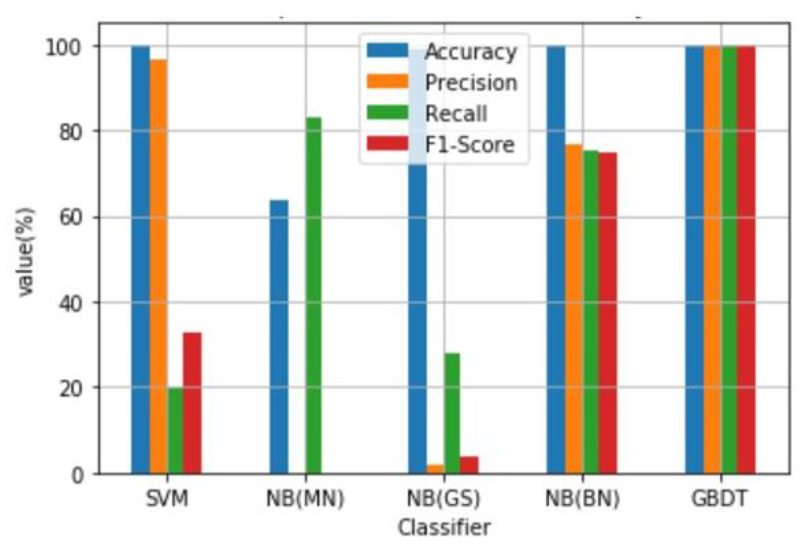
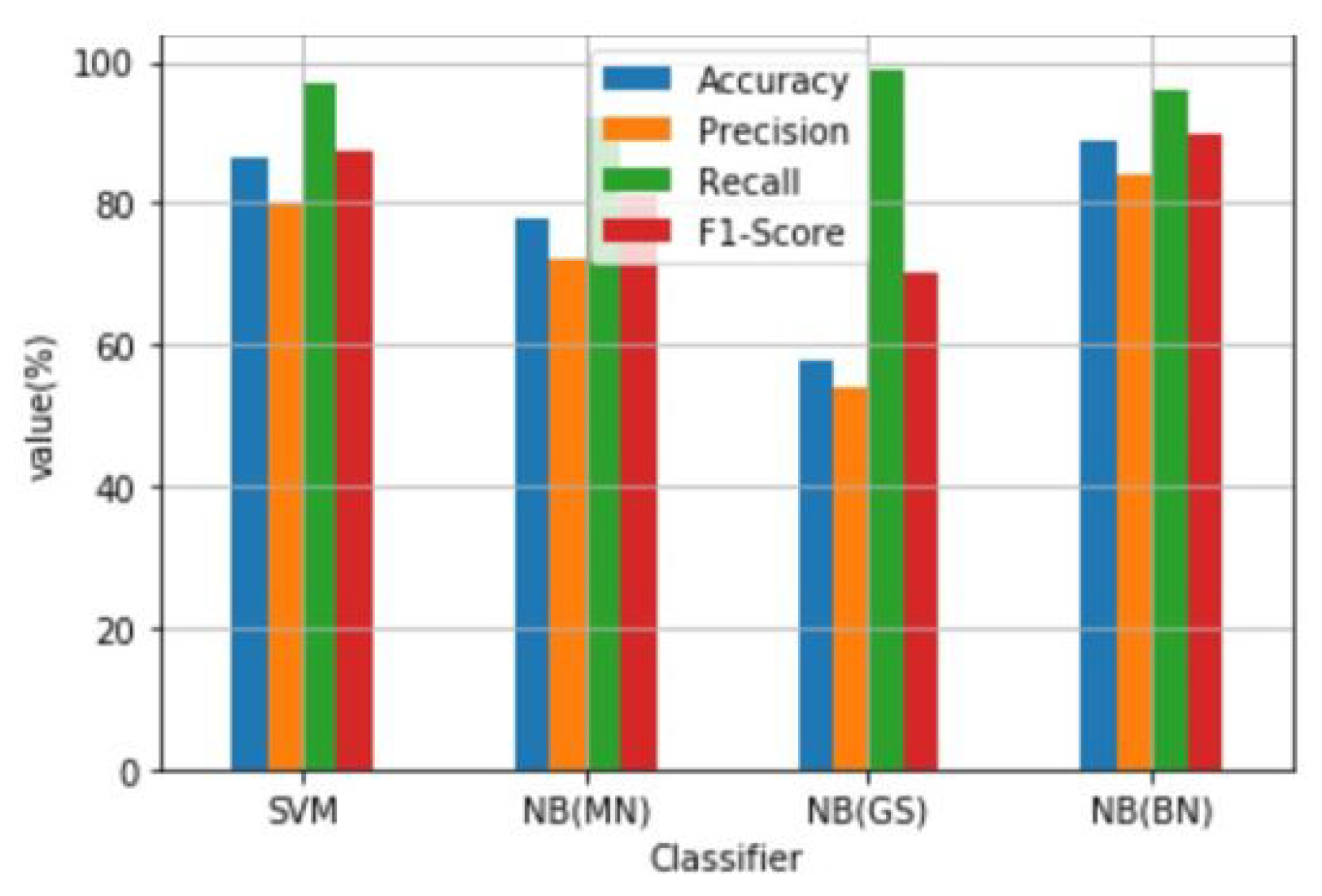
7.1. Results

This article investigated the effectiveness of three algorithms in predicting fraud in mobile money transactions; Support Vector Machines, Gradient Boosted Decision Trees, and Naïve Bayes Algorithms. For Naïve Bayes, we experimented all the types namely Multinomial, Gaussian and Bernoulli. We evaluated the performance of the algorithms based on accuracy, precision, recall and F1-Score since these metrics are great in evaluating classifications from imbalanced datasets. For support vector and Naïve Bayes Algorithms, we experimented two undersampling procedures, two oversampling methods and a combination of both undersampling and oversampling taking into account the imbalance nature of the dataset. GridSearchCV was employed to tune the hyperparameters. The results are reported in

Table 4. Classification report for SVM and Naïve Bayes (NB) without sampling of the dataset.

		Metric
Classifier	Accuracy (%)	Precision (%)	Recall (%)	F1-Score (%)
SVM	99.91	96.49	19.71	32.73
NB(MN)	63.83	0.00	83.00	0.00
NB(GS)	98.66	2.00	28.00	4.00
NB(BN)	99.90	76.79	75.31	74.97

,

Table 5. Classification report for SVM and NB with RandomUndersampler.

		Metric
Classifier	Accuracy (%)	Precision (%)	Recall (%)	F1-Score (%)
SVM	86.34	79.76	97.18	87.62
NB(MN)	77.93	72.00	92.00	81.00
NB(GS)	57.97	54.00	99.00	70.00
NB(BN)	88.97	84.00	96.00	90.00

,

Table 6. Classification report for SVM and NB with NearMiss.

		Metric
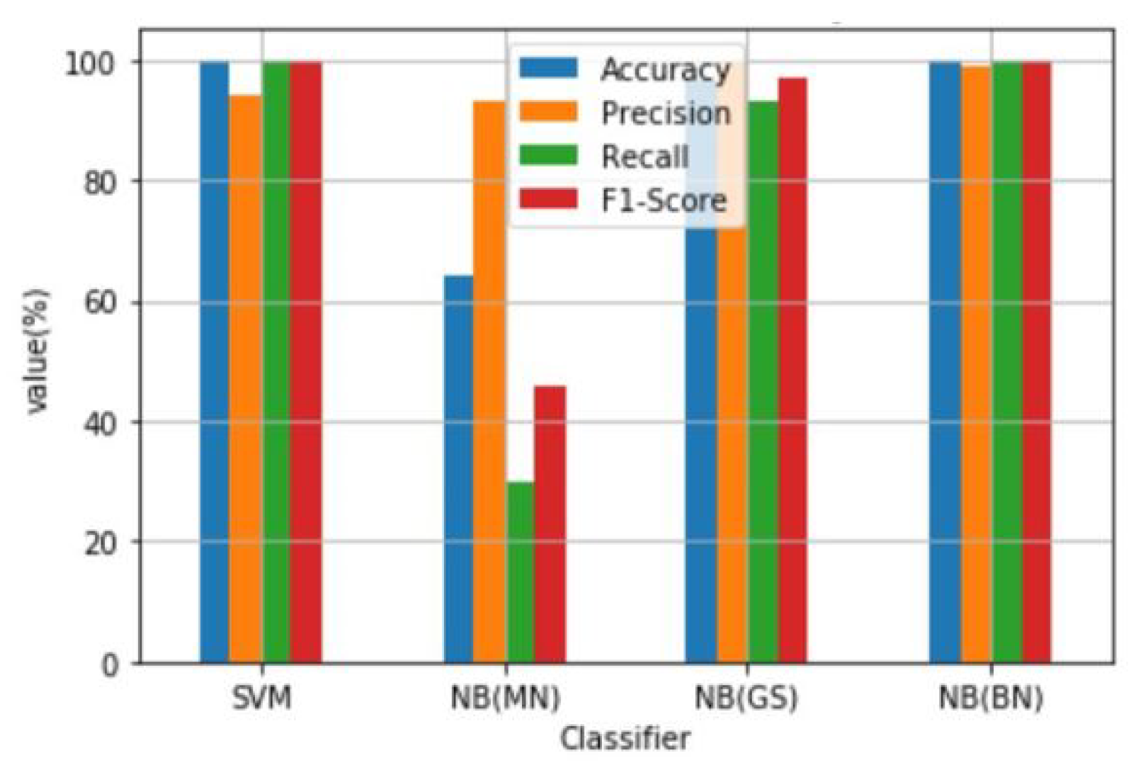
Classifier	Accuracy (%)	Precision (%)	Recall (%)	F1-Score (%)
SVM	99.64	93.90	100.00	99.65
NB(MN)	64.27	93.00	30.00	46.00
NB(GS)	96.67	100.00	93.00	97.00
NB(BN)	99.65	99.00	100.00	100.00

,

Table 7. Classification report for SVM and NB with RandomOverSampler.

		Metric
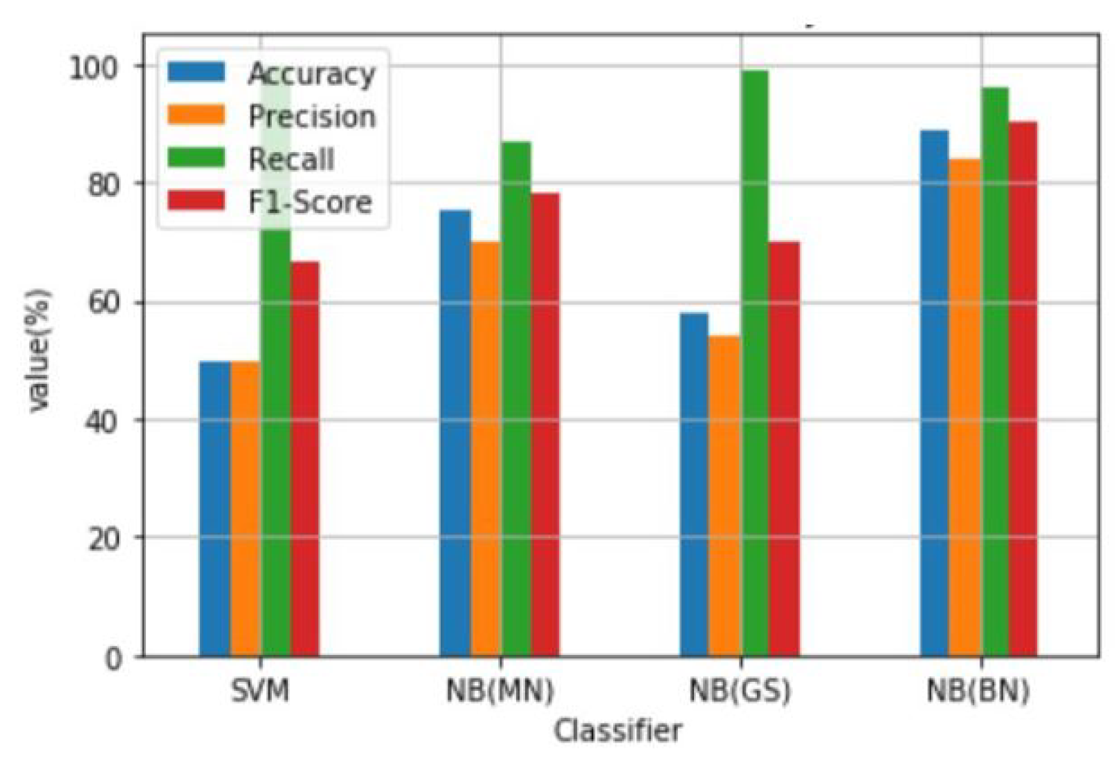
Classifier	Accuracy (%)	Precision (%)	Recall (%)	F1-Score (%)
SVM	49.87	49.77	100.00	66.47
NB(MN)	75.23	70.00	88.00	78.00
NB(GS)	57.97	54.00	99.00	70.00
NB(BN)	88.97	84.00	96.00	90.00

,

Table 8. Classification report for SVM and NB with SMOTE.

		Metric
Classifier	Accuracy (%)	Precision (%)	Recall (%)	F1-Score (%)
SVM	49.87	49.87	100.00	66.47
NB(MN)	75.30	70.00	87.00	78.00
NB(GS)	57.97	54.00	99.00	70.00
NB(BN)	88.97	84.00	96.00	90.00

and

Table 9. Classification report for SVM and NB with SMOTETomek.

		Metric
Classifier	Accuracy (%)	Precision (%)	Recall (%)	F1-Score (%)
SVM	49.78	49.78	100.00	66.47
NB(MN)	75.27	70.00	87.00	78.00
NB(GS)	57.97	54.00	99.00	70.00
NB(BN)	88.97	84.00	96.00	90.00

with their corresponding boxplots as Figure 5, Figure 6, Figure 7, Figure 8, Figure 9 and Figure 10. The plot for

Table 10. Classification report for Gradient boosted decision tree.

		Metric
Classifier	Accuracy (%)	Precision (%)	Recall (%)	F1-Score (%)
GBDT	99.90	99.99	100.00	99.95

has been added to that of Figure 5 to aid in analysis since in the case of Gradient boosted decision trees, no sampling was performed as decision trees are able to inherently deal with the problem of imbalance datasets. The result are reported in Table 10. The results show that gradient boosted decision tress churned out results which are very good.

7.2. Discussion

A cross-case analysis of our results are performed. Table 4 present the results of the experiment performed on the unsampled dataset. Even though the algorithms produced accuracy score in the range of 63.83% for Naïve Bayes (NB) using Multinomial (MN) to that of SVM of 00.91% which are pretty good, the F1-Scores produced were discouraging with NB (MN) producing 0.00% and NB Bernoulli (BN) producing 74.97% giving the range for that measure. F1-Score is one of the most important metric use for measuring the performance of imbalanced datasets because of its ability to balance recall and precision [55]. The F1-Score from this experiment is an indication that the results produced from imbalanced dataset without any sampling procedure are unreliable. The precision produced mixed results with the lowest of 0.00% coming from NB (MN) and highest 96.49% from SVM. In all, if F1-Score is considered as the most important metric, then NB (BN) can be considered as the best performing algorithm followed by SVM, NB(GS) and the worse algorithm being NB(MN). However, less emphasis is laid on the results presented in Table 4 for the preferred classifier due to the imbalanced nature of the dataset. Table 5 presents the classification report from the experiment from the first undersampling process; RandomUnderSampler. This experiment produced fairly good results with the accuracy ranging from 57.97% for NB Gaussian (GS) to 88.97% for NB (BN). The precision also ranged between 54.00% for NB (GS) to 84.00% for NB (BN) and very good recall of 92.00% NB (MN) to 99.00% for NB (GS). We, again, consider NB (BN) as the best performing classifier in the experiment producing F1-Score of 90.00% and NB (GS), NB (MN), and SVM obtaining 70.00%, 80.00%, and 87.62% respectively. Moreover, due to the fact that a chunk of information was lost through this process via undersampling, less emphasis is laid on this result but presents for analysis to obtain a holistic picture of the experiment performed. Table 6 presents the classification report for the second undersampling procedure; NearMiss. Comparing the results obtained from RandomUnderSampling to NearMiss, it was observed that the results from NearMiss are superior to that of RandomUnderSampler with an exception to the results from NB (MN) obtaining 30.00% for recall and 46.00% for F1-Scorein NearMiss compared to that of 92.00% and 81.00% for RandomUnderSampler. The rest of the results produced quite good results; accuracy 64.27% to 99.65%, precision from 93.00% to 100.00%, recall of 30.00% to 100.00% and F1-Score of 46.00% to 100.00%. Under NearMiss, NB(BN)is considered as the best performing classifier, followed by SVM and NB (GS) with NB (MN) coming up again as the worse performing classifier. It is observed from the two undersampling methods that the result produced are quite significant. Also, NB(BN), SVM, and NB(GS) performed well in both two cases with NB(MN) being the worse. Again, little importance was attached from the results obtained from our undersampling procedures since the procedure has the effect of throwing away a chunk of information from the dataset. However, the results obtained from undersampling are quite good. Table 7 and Table 8 present the classification report from the two oversampling experiments namely RandomOverSampler and SMOTE respectively. We also present the report from Table 9 which is the report form the combination of undersampling and oversampling; SMOTETomek. The report from these three experiments produced some interesting results, with all three producing similar results with most having differences appearing only in the decimal range.The accuracy ranged from 49.87% for SVM, 57.9 % for NB (GS), 75.23% for NB (MN) and 88.97% for NB (BN). The F1-Score also ranged from 66.47% for SVM to 90.00% for NB (BN). The results are quite similar to the other oversampling procedure SMOTE. It was observed that NB(BN) continued with its dominance as the best performing classifier in all the above discussions producing the best results in comparison to the other algorithms, having achieved its lowest mark in accuracy of 88.97%, precision of 84.00%, recall of 96.00% and the highest of 90.00% for F1-Score. SVM which performed pretty well previously did not do so well in the oversampling process. Also, NB(MN) which performed poorly in the two undersampling methods performed well in the oversampling methods. Table 9 which is the report from SMOTETomek followed the pattern of the two oversampling methods. Table 10, presents the classification report from the experiment performed with gradient boosted decision trees (GBDT). This experiment produced a near perfect result for accuracy, precision, recall and F1-Score with the values of 99.90%, 99.99%, 100.00%, and 99.95% respectively.

8. Conclusions

In this paper, the researchers performed experiments to determine the performance of support vector machines (kernel-based), gradient boosted decision tree (tree-based) and Naïve Bayes (probabilistic based) algorithms in prediction fraud in Mobile Money transactions, which is prevalent in developing countries. The results from the experiments were analyzed based on accuracy, precision, recall, and F1-Score which are considered as pretty good metrics for accessing the performance of classification algorithms from imbalanced datasets. The results from our experiments showed that the ensemble method; gradient boosted decision tree has the ability to adequately predict fraudulent transactions in MMTs. Also Bernoulli Naïve Bayes did perform pretty well in our the experiments.

References

- Guo, J.; Bouwman, H. An ecosystem view on third party mobile payment providers: A case study of Alipay wallet. Info 2016, 18, 56–78. [Google Scholar] [CrossRef] [Green Version]
- Cao, Q.; Niu, X. Integrating context-awareness and UTAUT to explain Alipay user adoption. Int. J. Ind. Ergon. 2019, 69, 9–13. [Google Scholar] [CrossRef]
- Akomea-Frimpong, I.; Andoh, C.; Akomea-Frimpong, A.; Dwomoh-Okudzeto, Y. Control of fraud on mobile money services in Ghana: An exploratory study. J. Money Laund. Control 2019, 22, 300–317. [Google Scholar] [CrossRef]
- Available online: https://www.ghanaweb.com/GhanaHomePage/NewsArchive/Momo-fraud-How-scammers-steal-your-money-791051 (accessed on 5 June 2020).
- Available online: https://www.graphic.com.gh/business/business-news/ghana-news-momo-fraud-threatens-emerging-payment-technologies.html (accessed on 5 June 2020).
- Available online: https://www.ghanabusinessnews.com/2019/09/18/mtn-ghana-tackles-mobile-money-fraud (accessed on 5 June 2020).
- de Sá, A.G.; Pereira, A.C.; Pappa, G.L. A customized classification algorithm for credit card fraud detection. Eng. Appl. Artif. Intell. 2018, 72, 21–29. [Google Scholar] [CrossRef]
- Hajek, P.; Henriques, R. Mining corporate annual reports for intelligent detection of financial statement fraud–A comparative study of machine learning methods. Knowl.-Based Syst. 2017, 128, 139–152. [Google Scholar] [CrossRef]
- Sadgali, I.; Sael, N.; Benabbou, F. Performance of machine learning techniques in the detection of financial frauds. Procedia Comput. Sci. 2019, 148, 45–54. [Google Scholar] [CrossRef]
- Singh, G.; Gupta, R.; Rastogi, A.; Chandel, M.D.; Ahmad, R. A machine learning approach for detection of fraud based on svm. Int. J. Sci. Eng. Technol. 2012, 1, 192–196. [Google Scholar]
- Jurgovsky, J.; Granitzer, M.; Ziegler, K.; Calabretto, S.; Portier, P.E.; He-Guelton, L.; Caelen, O. Sequence classification for credit-card fraud detection. Expert Syst. Appl. 2018, 100, 234–245. [Google Scholar] [CrossRef]
- Ryman-Tubb, N.F.; Krause, P.; Garn, W. How Artificial Intelligence and machine learning research impacts payment card fraud detection: A survey and industry benchmark. Eng. Appl. Artif. Intell. 2018, 76, 130–157. [Google Scholar] [CrossRef]
- Kotsiantis, S.; Koumanakos, E.; Tzelepis, D.; Tampakas, V. Forecasting fraudulent financial statements using data mining. Int. J. Comput. Intell. 2006, 3, 104–110. [Google Scholar]
- Pumsirirat, A.; Yan, L. Credit card fraud detection using deep learning based on auto-encoder and restricted boltzmann machine. Int. J. Adv. Comput. Sci. Appl. 2018, 9, 18–25. [Google Scholar] [CrossRef]
- Randhawa, K.; Loo, C.K.; Seera, M.; Lim, C.P.; Nandi, A.K. Credit card fraud detection using AdaBoost and majority voting. IEEE Access 2018, 6, 14277–14284. [Google Scholar] [CrossRef]
- Tran, P.H.; Tran, K.P.; Huong, T.T.; Heuchenne, C.; HienTran, P.; Le, T.M.H. Real time data-driven approaches for credit card fraud detection. In Proceedings of the 2018 International Conference on E-Business and Applications, Da Nang, Vietnam, 23–25 February 2018; pp. 6–9. [Google Scholar]
- Wang, C.; Wang, Y.; Ye, Z.; Yan, L.; Cai, W.; Pan, S. Credit card fraud detection based on whale algorithm optimized BP neural network. In Proceedings of the 2018 13th International Conference on Computer Science & Education (ICCSE), Colombo, Sri Lanka, 8–11 August 2018; pp. 1–4. [Google Scholar]
- Akila, S.; Reddy, U.S. Cost-sensitive Risk Induced Bayesian Inference Bagging (RIBIB) for credit card fraud detection. J. Comput. Sci. 2018, 27, 247–254. [Google Scholar] [CrossRef]
- Husejinovic, A. Credit card fraud detection using naive Bayesian and C4.5 decision tree classifiers. Period Eng. Nat. Sci. 2020, 8, 1–5. [Google Scholar]
- Adedoyin, A.; Kapetanakis, S.; Samakovitis, G.; Petridis, M. Predicting fraud in mobile money transfer using case-based reasoning. In Artificial Intelligence XXXIV: 37th SGAI International Conference on Innovative Techniques and Applications of Artificial Intelligence, AI 2017, Cambridge, UK, 12–14 December 2017; Springer: Berlin/Heidelberg, Germany, 2017; pp. 325–337. [Google Scholar]
- Fiore, U.; De Santis, A.; Perla, F.; Zanetti, P.; Palmieri, F. Using generative adversarial networks for improving classification effectiveness in credit card fraud detection. Inf. Sci. 2019, 479, 448–455. [Google Scholar] [CrossRef]
- Carcillo, F.; Le Borgne, Y.A.; Caelen, O.; Kessaci, Y.; Oblé, F.; Bontempi, G. Combining unsupervised and supervised learning in credit card fraud detection. Inf. Sci. 2019. [Google Scholar] [CrossRef]
- Awoyemi, J.O.; Adetunmbi, A.O.; Oluwadare, S.A. Credit card fraud detection using machine learning techniques: A comparative analysis. In Proceedings of the 2017 International Conference on Computing Networking and Informatics (ICCNI), Lagos, Nigeria, 29–31 October 2017; pp. 1–9. [Google Scholar]
- Varmedja, D.; Karanovic, M.; Sladojevic, S.; Arsenovic, M.; Anderla, A. Credit Card Fraud Detection-Machine Learning methods. In Proceedings of the 2019 18th International Symposium INFOTEH-JAHORINA (INFOTEH), East Sarajevo, Bosnia and Herzegovina, 20–22 March 2019; pp. 1–5. [Google Scholar]
- Vincent, P.; Larochelle, H.; Lajoie, I.; Bengio, Y.; Manzagol, P.A.; Bottou, L. Stacked denoising autoencoders: Learning useful representations in a deep network with a local denoising criterion. J. Mach. Learn. Res. 2010, 11, 3371–3408. [Google Scholar]
- Wah, Y.B.; Rahman, H.A.A.; He, H.; Bulgiba, A. Handling imbalanced dataset using SVM and k-NN approach. AIP Conf. Proc. 2016, 1750, 020023. [Google Scholar]
- Fernández, A.; Garcia, S.; Herrera, F.; Chawla, N.V. SMOTE for learning from imbalanced data: Progress and challenges, marking the 15-year anniversary. J. Artif. Intell. Res. 2018, 61, 863–905. [Google Scholar]
- Gosain, A.; Sardana, S. Handling class imbalance problem using oversampling techniques: A review. In Proceedings of the 2017 International Conference on Advances in Computing, Communications and Informatics (ICACCI), Udupi, India, 13–16 September 2017; pp. 79–85. [Google Scholar]
- Sundarkumar, G.G.; Ravi, V.; Siddeshwar, V. One-class support vector machine based undersampling: Application to churn prediction and insurance fraud detection. In Proceedings of the 2015 IEEE International Conference on Computational Intelligence and Computing Research (ICCIC), Madurai, India, 10–12 December 2015; pp. 1–7. [Google Scholar]
- Hossin, M.; Sulaiman, M. A review on evaluation metrics for data classification evaluations. Int. J. Data Min. Knowl. Manag. Process 2015, 5, 1–11. [Google Scholar]
- Available online: https://www.afi-global.org (accessed on 17 July 2020).
- Available online: https://www.gsma.com/mobilemoney (accessed on 17 July 2020).
- Payment System Statistics. Available online: https://www.bog.gov.gh (accessed on 18 July 2020).
- 2017 Findex full report_chapter2.pdf. Available online: https://globalfindex.worldbank.org (accessed on 18 July 2020).
- Hssina, B.; Merbouha, A.; Ezzikouri, H.; Erritali, M. A comparative study of decision tree ID3 and C4.5. Int. J. Adv. Comput. Sci. Appl. 2014, 4, 13–19. [Google Scholar] [CrossRef] [Green Version]
- Gokgoz, E.; Subasi, A. Comparison of decision tree algorithms for EMG signal classification using DWT. BioMed. Signal Process. Control 2015, 18, 138–144. [Google Scholar] [CrossRef]
- Farid, D.M.; Zhang, L.; Rahman, C.M.; Hossain, M.A.; Strachan, R. Hybrid decision tree and naïve Bayes classifiers for multi-class classification tasks. Expert Syst. Appl. 2014, 41, 1937–1946. [Google Scholar] [CrossRef]
- Si, S.; Zhang, H.; Keerthi, S.; Mahajan, D.; Dhillon, I.; Hsieh, C.J. Gradient boosted decision trees for high dimensional sparse output. In Proceedings of the 34th International conference on machine learning, Sydney, Australia, 6–11 August 2017. [Google Scholar]
- Martinek, P.; Krammer, O. Optimising pin-in-paste technology using gradient boosted decision trees. Solder. Surf. Mt. Technol. 2018, 30, 164–170. [Google Scholar] [CrossRef]
- Wen, Z.; He, B.; Kotagiri, R.; Lu, S.; Shi, J. Efficient gradient boosted decision tree training on GPUs. In Proceedings of the 2018 IEEE International Parallel and Distributed Processing Symposium (IPDPS), Vancouver, BC, Canada, 21–25 May 2018; pp. 234–243. [Google Scholar]
- Saritas, M.M.; Yasar, A. Performance analysis of ANN and Naive Bayes classification algorithm for data classification. Int. J. Intell. Syst. Appl. Eng. 2019, 7, 88–91. [Google Scholar] [CrossRef] [Green Version]
- Li, T.; Li, J.; Liu, Z.; Li, P.; Jia, C. Differentially private Naive Bayes learning over multiple data sources. Inf. Sci. 2018, 444, 89–104. [Google Scholar] [CrossRef]
- Lopez-Rojas, E.; Elmir, A.; Axelsson, S. PaySim: A financial mobile money simulator for fraud detection. In Proceedings of the 28th European Modeling and Simulation Symposium, EMSS, Larnaca, Cyprus, 26–28 September 2016; pp. 249–255. [Google Scholar]
- Available online: https://imbalanced-learn.readthedocs.io/en/stable/generated/imblearn.under_sampling.RandomUnderSampler.html (accessed on 5 June 2020).
- Mani, I.; Zhang, I. kNN approach to unbalanced data distributions: A case study involving information extraction. In Proceedings of the Workshop on Learning from Imbalanced Datasets, Washington, DC, USA, 21 August 2003; Volume 126. [Google Scholar]
- Devi, D.; Purkayastha, B. Redundancy-driven modified Tomek-link based undersampling: A solution to class imbalance. Pattern Recognit. Lett. 2017, 93, 3–12. [Google Scholar] [CrossRef]
- Batista, G.E.; Prati, R.C.; Monard, M.C. A study of the behavior of several methods for balancing machine learning training data. ACM SIGKDD Explor. Newsl. 2004, 6, 20–29. [Google Scholar] [CrossRef]
- Pereira, R.M.; Costa, Y.M.; Silla, C.N., Jr. MLTL: A multi-label approach for the Tomek Link undersampling algorithm. Neurocomputing 2020, 383, 95–105. [Google Scholar] [CrossRef]
- Available online: https://imbalanced-learn.readthedocs.io/en/stable/generated/imblearn.over_sampling.RandomOverSampler.html (accessed on 5 June 2020).
- Chawla, N.V.; Bowyer, K.W.; Hall, L.O.; Kegelmeyer, W.P. SMOTE: Synthetic minority over-sampling technique. J. Artif. Intell. Res. 2002, 16, 321–357. [Google Scholar] [CrossRef]
- Available online: https://www.geeksforgeeks.org/ml-handling-imbalanced-data-with-smote-and-near-miss-algorithm-in-python/ (accessed on 21 July 2020).
- de Morais, R.F.; Vasconcelos, G.C. Boosting the performance of over-sampling algorithms through under-sampling the minority class. Neurocomputing 2019, 343, 3–18. [Google Scholar] [CrossRef]
- Wang, Z.; Wu, C.; Zheng, K.; Niu, X.; Wang, X. SMOTETomek-Based Resampling for Personality Recognition. IEEE Access 2019, 7, 129678–129689. [Google Scholar] [CrossRef]
- Boardman, J.; Biron, K.; Rimbey, R. Mitigating the Effects of Class Imbalance Using SMOTE and Tomek Link Undersampling in SAS®. Available online: https://pdfs.semanticscholar.org/bf3e/68c3e9cfe50b75897d6e6296c45f5bd30f82.pdf (accessed on 31 July 2020).
- Liu, T.; Wang, S.; Wu, S.; Ma, J.; Lu, Y. Predication of wireless communication failure in grid metering automation system based on logistic regression model. In Proceedings of the 2014 China International Conference on Electricity Distribution (CICED), Shenzhen, China, 23–26 September 2014; pp. 894–897. [Google Scholar]