Measurement of Text Similarity: A Survey

Abstract

Text similarity measurement is the basis of natural language processing tasks, which play an important role in information retrieval, automatic question answering, machine translation, dialogue systems, and document matching. This paper systematically combs the research status of similarity measurement, analyzes the advantages and disadvantages of current methods, develops a more comprehensive classification description system of text similarity measurement algorithms, and summarizes the future development direction. With the aim of providing reference for related research and application, the text similarity measurement method is described by two aspects: text distance and text representation. The text distance can be divided into length distance, distribution distance, and semantic distance; text representation is divided into string-based, corpus-based, single-semantic text, multi-semantic text, and graph-structure-based representation. Finally, the development of text similarity is also summarized in the discussion section.

1. Introduction

From the point of view of information theory [1], similarity is defined as the commonness between two text snippets. The greater the commonness, the higher the similarity, and vice versa. Text similarity is fast becoming a key instrument in many NLP (Natural Language Processing) based tasks, such as information retrieval [2], automatic question answering [3], machine translation [4], dialogue systems [5], and document matching [6].

Measures of various semantic similarity techniques have been proposed over the past three decades. Most scholars divide text similarity measurement methods on the basis of statistics or corpus and knowledge bases, such as Wikipedia [7]. This classification ignores the text distance calculation method, and only considers the representation of the text. Meanwhile, with the development of neural network representation learning, some semantic matching methods and graph methods need to be considered.

Text similarity not only accounts for the semantic similarity between texts but also considers a broader perspective analyzing the shared semantic properties of two words. For example, the words ‘King’ and ‘man’ may be related to one another closely, but they are not considered semantically similar whereas the words ‘King’ and ‘Queen’ are semantically similar. Thus, semantic similarity may be considered as one of the aspects of semantic relatedness. The semantic relationship including similarity is measured in terms of semantic distance, which is inversely proportional to the relationship.

Motivation of the Survey

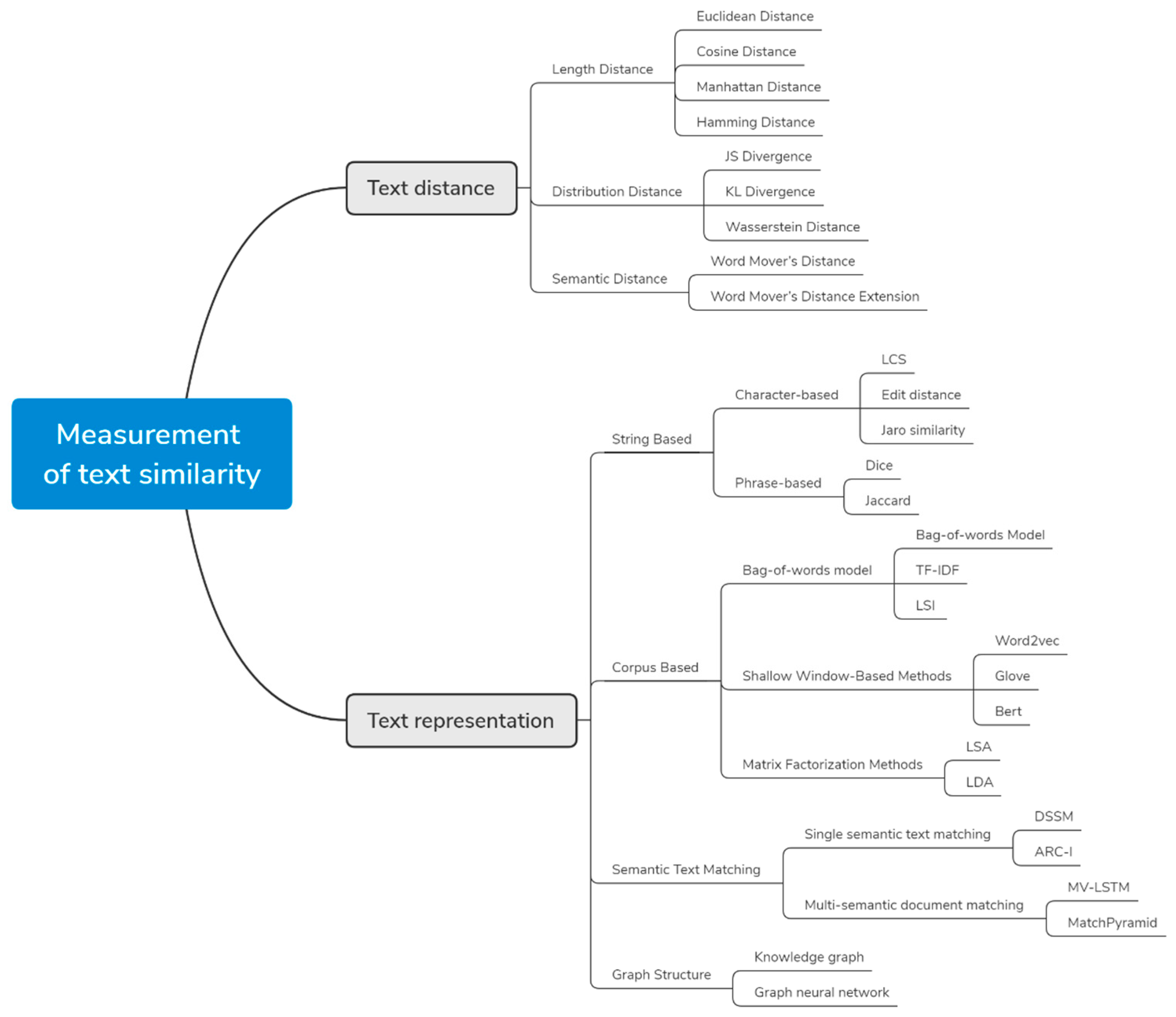
Most of the previous methods draw lessons from the classification framework of Gomaa et al. [7] to study the influence of word-based text representation on semantic similarity. This paper makes a further extension and subdivision of the classification system. The contribution of this survey is that it traces the evolution of semantic similarity technologies over the past few decades, distinguishing them based on the underlying methods used in them. Figure 1 shows the structure of the survey. The similarity calculation is divided into text distance and text representation: (a) Text distance describes the semantic proximity of two text words from the perspective of distance, including: length distance, distribution distance, and semantic distance. (b) Text representation represents the text as numerical features that can be calculated directly, including: the string-based method, corpus-based method, semantic text matching, and the graph-structure-based method. Different methods of text distance for semantic similarity are introduced in Section 2. Section 3 provides a detailed description of semantic similarity methods. Section 4 and Section 5 summarize the methods the in survey. This survey provides a deep and wide knowledge of existing techniques for new researchers who venture into exploring one of the most challenging NLP tasks, textual similarity.

2. Text Distance

The first section of this paper will examine the text distance, which describes the semantic proximity of two text words from the perspective of distance. There are three ways of measuring distance according to the length, distribution, and semantics of the object: length distance, distribution distance, and semantic distance.

2.1. Length Distance

Traditionally, text similarity has been assessed by measuring length distance, which uses the numerical characteristics of text to calculate the distance length of vector text. The most popular for each type will be presented briefly.

2.1.1. Euclidean Distance

Mathematically, the Euclidean distance is the straight line distance between two points in Euclidean space [8]. The Euclidean space becomes a metric space with the distance.

$$d(S_a,S_b)=\sqrt{{\displaystyle \sum }_{i=1}^n{(S_a^{(i)}-S_b^{(i)})}^2}$$

(1)

2.1.2. Cosine Distance

When measuring the cosine distance, instead of measuring the distance between the two points, it is transformed into the angle problem corresponding to the two points in the vector space. Similarity is calculated by measuring the cosine of the angle between two vectors [8].

Because of the size of the document, even if two similar documents are far away from Euclid, it is more advantageous to use the cosine distance to measure similarity. This may also be used to compare the relevance of a document’s perspective.

$$\mathrm{Sim}(S_a,S_b)=\cos \mathsf{\Theta }=\frac{\overrightarrow{S_a}·\overrightarrow{S_b}}{||S_a||·||S_b||}$$

(2)

2.1.3. Manhattan Distance

The Manhattan distance is also used to calculate the distance between two real-valued vectors. Manhattan distance is calculated as the sum of the absolute differences between the two vectors, which generally works only if the points are arranged in the form of a grid and the problem that we are working on gives more priority to the distance between the points only along with the grids, but not the geometric distance. The similarity of two documents is obtained through Manhattan distance after one-hot encoding [8]. In the two-dimensional space, the Manhattan formula is as follows:

$$\mathrm{Sim}(\mathrm{x}, \mathrm{y})=|x_1-x_2|+|y_1-y_2|$$

(3)

2.1.4. Hamming Distance

Hamming distance is a metric for comparing two binary data strings. While comparing two binary strings of equal length, Hamming distance is the number of bit positions in which the two bits are different. The Hamming distance between two strings, a and b, is denoted as d (a, b). It is used for error detection or error correction when data is transmitted over computer networks. It is also used in coding theory for comparing equal length data words.

For binary strings A and B, this is equal to the number of times “1” occurs in binary strings [9].

2.2. Distribution Distance

There are two problems with using length distance to calculate similarity:

First, it is suitable for symmetrical problems, such as Sim (A, B) = Sim (B, A), but for question Q to retrieve answer A, the corresponding similarity is not symmetrical.

Second, there is a risk in using length and distance to judge similarity without knowing the statistical characteristics of the data [8].

The distribution distance is used to compare whether the documents come from the same distribution, so as to judge the similarity between documents according to the distribution. JS divergence and KL divergence are currently the most popular methods for investigating distribution distance.

2.2.1. JS Divergence

Jensen–Shannon divergence is a method to measure the similarity between two probability distributions. It is also known as the information radius (IRAD) or the total divergence to the average [10].

JS divergence is usually used in conjunction with LDA (latent dirichlet allocation) to compare the topic distribution of new documents with all topic distributions of documents in the corpus and to determine which documents are more similar in distribution by comparing their distribution differences. The smaller the Jensen–Shannon distance, the more similar the distribution of the two documents [11].

Assume that two documents belong to two different distributions P₁ and P₂, the JS divergence formula is as follows:

$$\mathrm{JS}(P_1\Vert P_2)=\frac{1}{2}KL(P_1\Vert \frac{P_1+P_2}{2})+\frac{1}{2}KL(P_2\Vert \frac{P_1+P_2}{2})$$

(4)

2.2.2. KL Divergence

Kullback–Leibler divergence (also known as relative entropy) is a measure of different degrees of a probability distribution and a second reference probability distribution [12].

Let p (x) and q (x) be two probability distributions with values of X, then the relative entropy of p to q is:

$$\mathrm{d}(\mathrm{p}\Vert \mathrm{q})={\displaystyle \sum }_{i=1}^{n}p(x)log\frac{p(x)}{q(x)}$$

(5)

2.2.3. Wasserstein Distance

Wasserstein distance is a measure of the distance between two probability distributions [13]. When the two distributed support sets do not overlap or overlap very little, the result of the KL divergence is infinite and the JS divergence is non-differentiable at 0, while the Wasserstein distance can provide smoother results for updating the parameters of the gradient descent method. It is defined as follows:

$$W(p_r,p_g)=\underset{\gamma ~{\displaystyle \prod (p_r,p_g)}}{\inf }{E}_{(x,y)~\gamma }[\Vert x-y\Vert ]$$

(6)

In the formula above, ${\prod }^{ }(p_r,p_g)$ is the set of all possible joint probability distributions between $p_r$ and $p_g$. One joint distribution γ ∈ $\prod (p_r,p_g)$ describes one dirt transport plan—the same as the discrete example above—but in the continuous probability space. Precisely γ(x, y) states the percentage of dirt should be transported from point x to y so as to make x follow the same probability distribution of y [14].

2.3. Semantic Distance

When there is no common word in the text, the similarity obtained by using the distance measure based on length or distribution may be relatively small, so we can consider calculating the distance at the semantic level. Word mover’s distance is the main method used to determine semantic distance [15].

2.3.1. Word Mover’s Distance

On the basis of representing the text as a vector space, word mover’s distance uses the method of earth mover’s distance [16] to measure the minimum distance required for a word in one text to reach a word in another text in the semantic space, so as to minimize the cost of transporting text 1 to text 2 [17].

Word mover’s distance is a method that uses transportation on the basis of a word vector, and its core is linear programming [15].

2.3.2. Word Mover’s Distance Extension

In word mover’s distance, Euclidean distance is used to calculate the similarity. Euclidean distance regards every dimension in a space as the same weight; that is, the importance of each dimension is the same. But the correlation between different dimensions is not taken into account. If you want to take this information into account, you can use the improved version of the distance called Mahalanobis distance [18] instead of the Euclidean distance; that is, make a linear transformation of the sample in the original space at first, and then calculate the Euclidean distance in the transformed space.

Through the introduction of matrix loss, the unsupervised word mover’s distance is transformed into supervised word mover’s distance, so that it can be applied to the task of text classification more efficiently [19].

3. Text Representation

The second section of this paper will examine the text representation, which represents the text as numerical features that can be calculated directly. Texts can be similar in two ways lexically and semantically. The words that make up the text are similar lexically if they have a similar character sequence. Words are similar semantically if they have the same thing, are opposite of each other, used in the same way, used in the same context, and one is a type of another. Lexical similarity is introduced in this survey though different measurements of text representation, semantic similarity is introduced through the string-based method, corpus-based method, semantic text matching, and graph-structure-based method.

3.1. String-Based

The advantages of string-based methods are that they are simple to calculate. String similarity measures operate on string sequences and character composition that measures similarity or dissimilarity (distance) between two text strings for approximate string matching or comparison. This survey represents the most popular string similarity measures, which were implemented in the symmetric package [1]. As shown in Figure 1, according to the basic units, different methods have been proposed to classify character-based methods and phrase-based methods. The most popular for each type will be presented briefly.

3.1.1. Character-Based

A character-based similarity calculation is based on the similarity between characters in the text to express the similarity between texts. Three algorithms will be introduced: LCS (longest common substring), editing distance, Jaro similarity, and so on.

• LCS

Thinking of the text as a string, LCS represents the length of the longest substring that is the same as the strings $S_a$ and $S_b$. There is more information in common between the long strings [20,21,22].

LCS [23] matching is a commonly used technique to measure the similarity between two strings ($S_a$, $S_b$). Thinking of the text as a string, LCS represents the length of the longest substring that is the same as the strings $S_a$ and $S_b$. There is more information in common between the long strings [15,16,17]. The LCS similarity of two given strings (i, j) will be:

$$\mathrm{LCS}(S_a,S_b)=\{\begin{array}{c}0, if S_a=0 or S_a=0\\ 1+LCS(S_a-1,S_b-1),if x\left[S_a\right]==y\left[S_b\right]\\ max\{\begin{array}{c}LCS(S_a,S_b-1)\\ LCS(S_a-1,S_b)\end{array}if x\left[S_a\left]\ne y\right[S_b\right]\end{array}$$

(7)

• Edit distance

The edit distance represents the minimum number of transformations required to convert the string from $S_a$ to $S_b$. There are two forms of definition of editing distance, which are L-distance [24] and D-distance [25].

Between them, the atomic operations of D-distance include delete, insert, replace, and adjacent exchange operations, while the atomic operations of L-distance only include delete, insert, and replace operations. Because there is one more adjacent operation in the definition of D-distance, the D-distance can only deal with a single editing error, while L-distance can handle multiple editing errors.

• Jaro similarity

For two strings $S_a$ and $S_b$, the Jaro similarity representation is as follows [26]:

$$\mathrm{Sim}=\{\begin{array}{c}0,if m=0\\ \frac{1}{3}(\frac{m}{|S_a|}+\frac{m}{|S_b|}+\frac{m-t}{m})\end{array}$$

(8)

where: |$S_a$| and |$S_b$| indicate the length of strings |$S_a$| and |$S_b$|, m represents the number of matching characters of two strings, and t represents half of the transposition number.

3.1.2. Phrase-Based

The difference between the phrase-based method and character-based method is that the basic unit of the phrase-based method is a phrase word, and the main methods are the dice coefficient, Jaccard, and so on.

• Dice

Where comm ($S_a$, $S_b$) indicates the number of collinear phrases, that is, the number of the same characters in the strings $S_a$ and $S_b$ [27].

$$\mathrm{Dice}(S_a,S_b)=\frac{2\times \mathrm{comm}(S_a,S_b)}{len(S_a)+len(S_b)}$$

(9)

• Jaccard

Jaccard similarity is defined as the size of the intersection divided by the size of the union of two sets [28].

Jaccard is to solve the similarity through the set; when the text is relatively long, the similarity will be smaller. Therefore, when Jaccard is used to calculate similarity, it is usually normalized at first. For English, words can be reduced to the same root, and for Chinese, words can be reduced to synonyms.

$$\mathrm{S}(S_a,S_b)=\frac{S_a{{\displaystyle \cap }}^{ }{S}_b}{S_a{{\displaystyle \cup }}^{ }{S}_b}$$

(10)

3.2. Corpus-Based

There is an important difference between corpus-based and string-based methods: The corpus-based method uses the information obtained from the corpus to calculate the text similarity; this information can be either a textual feature or a co-occurrence probability. However, the string-based approach is a text comparison at the literal level. In most recent studies, the corpus-based method has been measured in three different ways: bag-of-words model, distributed representation, and matrix factorization methods.

3.2.1. Bag-of-Words Model

The basic idea of the bag-of-words model is to represent the document as a combination of a series of words without considering the order in which words appear in the document [29]. The methods based on the word bag model mainly include BOW (bag of words), TF-IDF (term frequency–inverse document frequency), LSA (latent semantic analysis), and so on.

• BOW

The essence of BOW is count vectorization, which represents text by counting the number of words that appear in a document and then uses these word counts to measure similarity in applications, such as search, document classification, and topic modeling [30].

• TF-IDF

TF-IDF works because a word appears more often in a document, and there are a large number of documents containing that word. However, although the words frequently appear in a document, they have no special meaning to the document [31].

Calculation of the TF-IDF score for each word in the document set is as follows:

tf-idf (w, d, D) = tf (w, d) × idf (w, D)

(11)

where:

tf (w, d) = Freq (w, d)

(12)

$$idf (w, D ) = log\frac{|D|}{N(w)}$$

(13)

Freq (w, d) indicates how often a word is used in the document, |D| indicates the number of the document, and N (w) is the number of words that appear in the document. There is a TF-IDF representation for all the words in the document, and the number of words is equal to the number of words represented by TF-IDF.

3.2.2. Shallow Window-Based Methods

The shallow window-based methods differs from the word bag model in an important way is that the word bag model does not capture the semantic distance between words. However, by generating word vectors through shallow window-based methods, low-dimensional real vectors can be trained in unstructured text with no mark, which makes similar words closer in distance. At the same time, it solves the disaster of dimensionality and lack of semantics caused by the word bag model because of word independence.

A number of techniques have been developed to represent word vectors, there are three main methods of study: Word2vec and glove.

• Word2vec

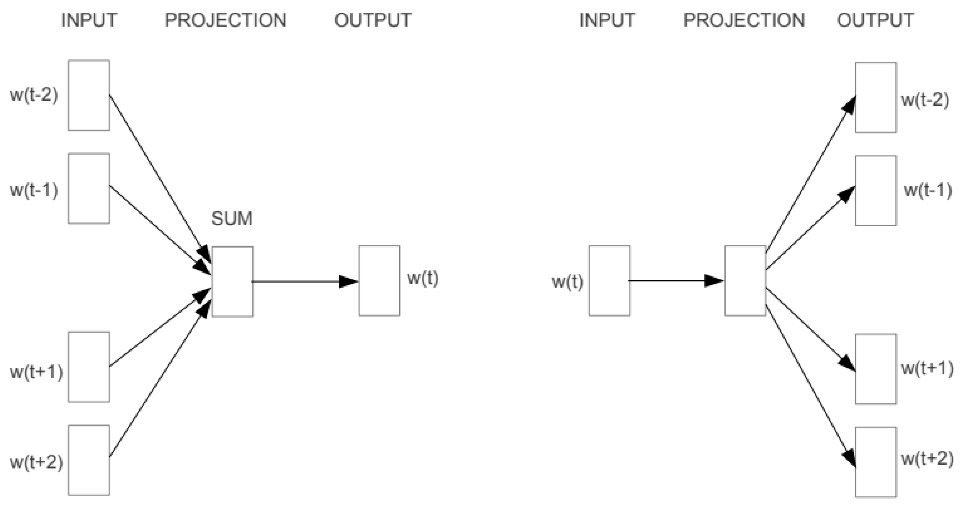
Word2Vec has two pre-training models, which are continuous word bag model (continuous bag of words, CBOW) and word-skipping model (skip-gram) [32]. Take the CBOW model as an example: the intermediate words are predicted according to the context, and this model includes the input layer, the mapping layer, and the output layer [33]. First of all, the model inputs the unique heat vector corresponding to the context of the inter-word. Then, all the unique heat vectors are multiplied by the shared input weight matrix W. Next, the word vectors are added to find the average as the hidden layer vector. Finally, the hidden layer vector is multiplied by the weight matrix W of the output, and the result is input into the SoftMax function to obtain the final probability distribution [34]. Skip-gram and CBOW of Word2vec measures are described in Figure 2.

• Glove

Glove is a word representation tool based on global word frequency statistics, which explains the semantic information of words by modeling the contextual relationship of words. Its core idea is that words with similar meanings often appear in similar contexts [35].

• BERT

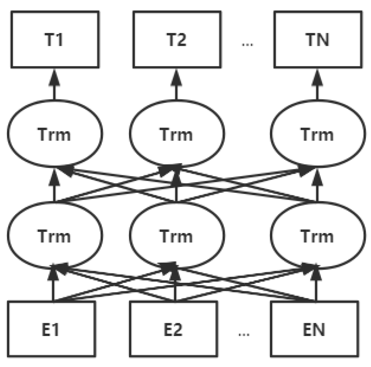
BERT’s full name is bidirectional encoder representation from transformers, because decoder is unable to capture the directional encoder representation from transformers. The main innovation of the model is based on the pre-train approach, which covers masked language model and next sentence prediction, which capture expression and sentence-level representation, respectively [36]. However, BERT will be complicated to obtain interactive computing when it is used, so it generally not used as a way of computing similarity text when facing downstream tasks. BERT’s model architectures are described in Figure 3.

3.2.3. Matrix Factorization Methods

Matrix factorization methods for generating low-dimensional word representations have roots stretching as far back as LSA (latent semantic analysis). These methods utilize low-rank approximations to decompose large matrices that capture statistical information about a corpus. The particular type of information captured by such matrices varies by application. Recent advances in LSA methods have facilitated investigation of LDA (latent dirichlet allocation) methods.

• LSA

On the basis of the comparatively similar degree of word bag vector, LSA (latent semantic analysis) [37,38] maps the text from sparse high-dimensional vocabulary space to low-dimensional latent semantic space by singular value decomposition, so as to calculate the similarity in the potential semantic space [39,40].

Assume that words with similar meanings will appear in similar text fragments. A matrix containing the number of words in each document (rows representing unique words and columns representing each document) is made up of a large piece of text. Singular value decomposition (SVD) is used to reduce the number of rows, while preserving the similarity structure between columns. The document is then compared by taking the cosine of the angle between the two vectors formed by any two columns. Values close to 1 represent very similar documents, while values close to 0 represent very different documents [41].

After that, Hofmann introduces the topic layer on the basis of LSA, using the expectation maximization algorithm (expectation maximization, EM) to train the topic and obtains the improved PLSA (probabilistic latent semantic analysis) algorithm [42].

• LDA

LDA (latent dirichlet allocation) assumes that each document will contain several topics, so there is an overlap of topics in the document. The words in each document contribute to these topics. Each document will have a discrete distribution on all topics, and each topic will have a discrete distribution on all words [43].

The model is initialized by assigning each word in each document to a random topic. Then, we iterate through each word, cancel the assignment to its current topic, reduce the corpus scope of the topic count, and reassign the word to a new topic on the basis of local probability that the topic is assigned to the current document as well as global (corpus scope) probability that the word is assigned to the current topic [44].

3.3. Semantic Text Matching

Semantic similarity [45] determines the similarity between text and document on the basis of their meaning rather than character by character matching. On the basis of LSA, the hierarchical semantic structure embedded in the query and document is extracted by deep learning. Here, the text is encoded to extract features, thus a new expression is obtained. Each of these measures is described in Figure 1 [46].

3.3.1. Single Semantic Text Matching

Single semantic text matching mainly includes DSSM (deep-structured semantic model), CDSSM (convolutional latent semantic model), ARC-I (Architecture-I for matching two sentences), and ARC-II (Architecture-II of convolutional matching model).

• DSSM

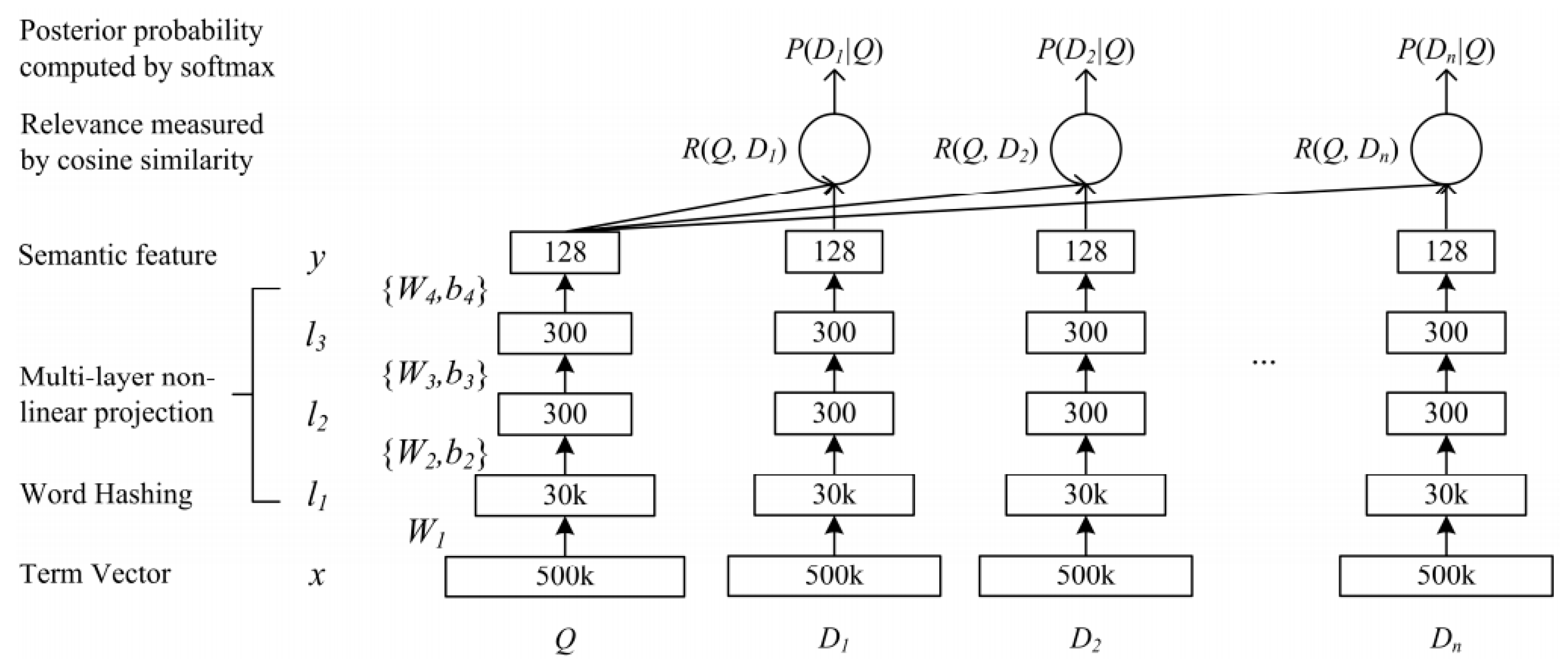
DSSM (deep-structured semantic models) was originally used in search business. The principle is that through the click exposure log of massive search results, Query and Title are expressed as low-latitude semantic vectors by DNN (Deep Neural Networks), the distance between the two semantic vectors is calculated by cosine distance, and finally the semantic similarity model is trained. Replacing DNN with CNN (Convolutional Neural Network), so that to some extent he can make up for the loss of context in DSSM [47]. The model can be used not only to predict the semantic similarity of two sentences but also obtain the low-latitude semantic vector representation of a sentence [48].

The DSSM is described in Figure 4. The model structure of DSSM is mainly divided into three parts: embedding layer, feature extraction layer, and SoftMax output layer.

(a)

The embedding layer mainly includes: TermVector and WordHashing. TermVector uses the bag-of-words model, but this can easily lead to OOV (out of vocabulary) problems. Then, it uses word hashing to combine words with n-gram, which effectively reduces the possibility of OOV.

(b)

The feature extraction layer mainly includes: Multi-layer, semantic feature, cosine similarity. Its main function is to extract the semantic feature of two text sequences through three full connection layers to calculate the cosine similarity.

(c)

The similarity is judged by the output layer through SoftMax binary classification.

With the development of deep learning, CNN and long and short-term memory (LSTM) [49] are proposed, and the structures of these special diagnosis extraction are also applied to DSSM. The main difference is that the full connection structure of the feature extraction layer is replaced by CNN or LSTM.

• ARC-I

In view of the deficiency of the DSSM model mentioned above in capturing query and doc sequences and context information, the CNN module is added to the DSSM model, thus ARC-I and ARC-II are proposed. ARC-I is a representation learning-based model, and the ARC-II model belongs to the interactive learning model. Through n-gram convolution extraction of word in query and convolution extraction of word in doc, the word vectors obtained by convolution are calculated by pairwise, then a matching degree matrix is obtained.

Compared with the original DSSM model, the most important feature of the two models is that convolution and pooling layers are introduced to capture the word order information in sentences [50].

Architecture-I (ARC-I) is illustrated in Figure 5. It obtains multiple combinatorial relationships between adjacent feature maps by convolution layer with different term, then the most important parts of these combinatorial relationships are extracted by pooling layer maxpooling. Finally, DSSM will get the representation of the text.

3.3.2. Multi-Semantic Document Matching

When complex sentences are compressed into a single vector based on single semantics, important local information will be lost. On the basis of single semantics, the deep learning model of document expression based on multi-semantics proposes that a single-granularity vector to represent a piece of text is not fine enough. It requires multi-semantic expression and does a lot of interactive work before matching, so that we can do some local similarity and synthesize the matching degree between texts. The main multi-semantic methods are: multi-view bi-LSTM (MV-LSTM) and MatchPyramid.

• MV-LSTM

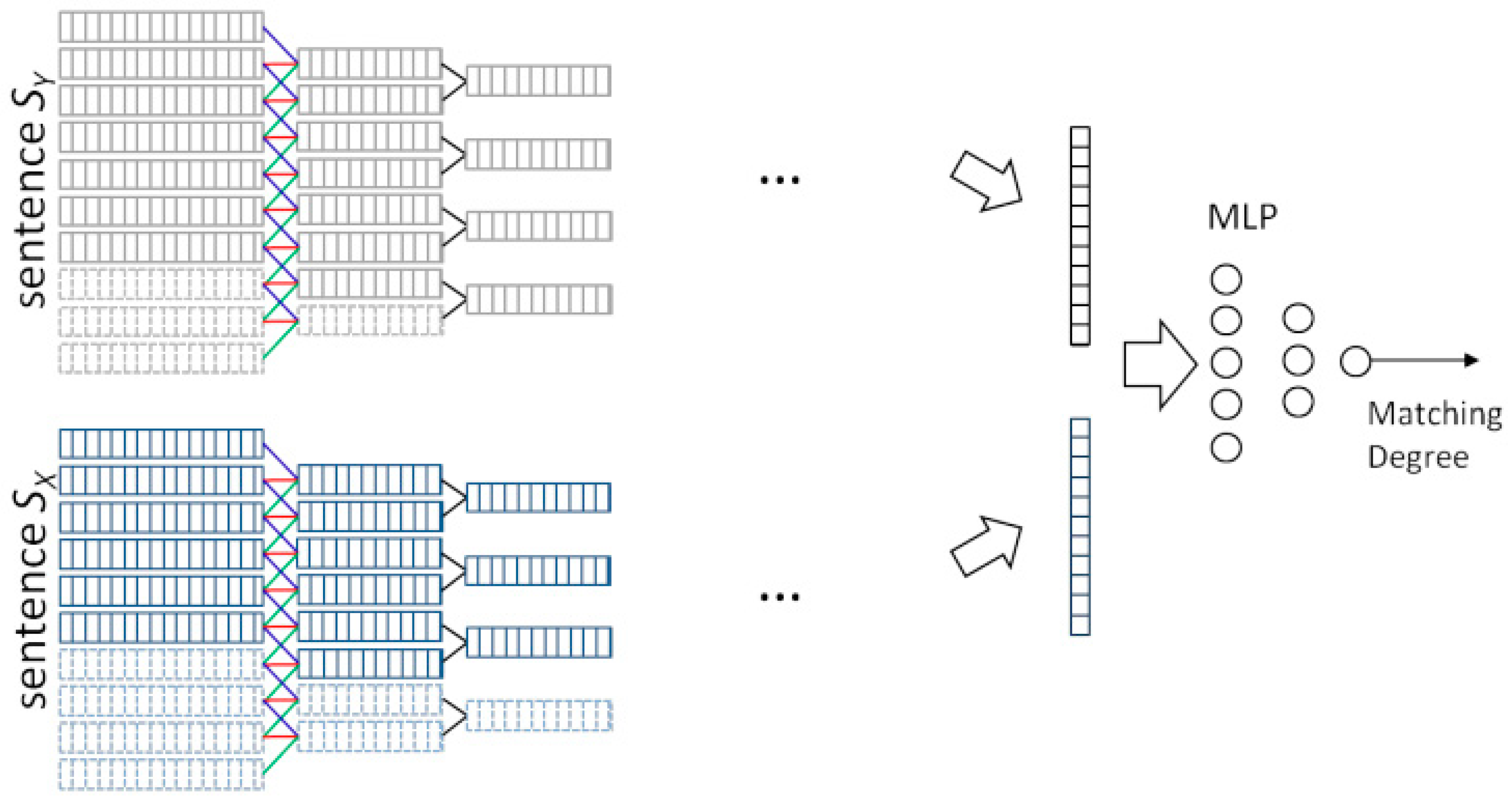
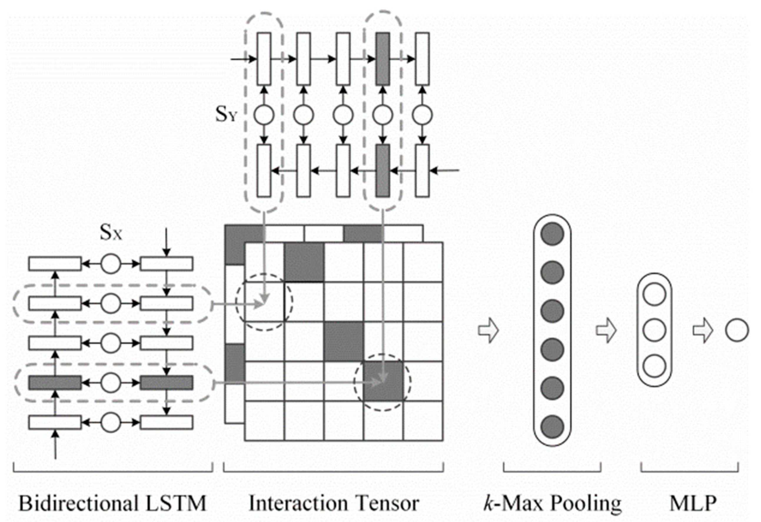
MV-LSTM (multi-view bi-LSTM) uses bidirectional long and short-term memory (Bi-LSTM) to generate positional sentence representations. Specifically, for each location, Bi-LSTM can get two hidden vectors to reflect the content meaning in both directions at this location [51].

Through the introduction of multiple positional sentence representations, important local information can be well captured with the importance of local information can be determined by using rich context information. MV-LSTM is illustrated in Figure 6.

$S_X$ and $S_Y$ are the input sentences. Positional sentence representations (denoted as the dashed orange box) are first obtained by a Bi-LSTM. K-Maximum pooling then selects the top k interactions from each interaction matrix (denoted as the blue grids in the graph). The matching score is finally computed through a multilayer perceptron.

• MatchPyramid

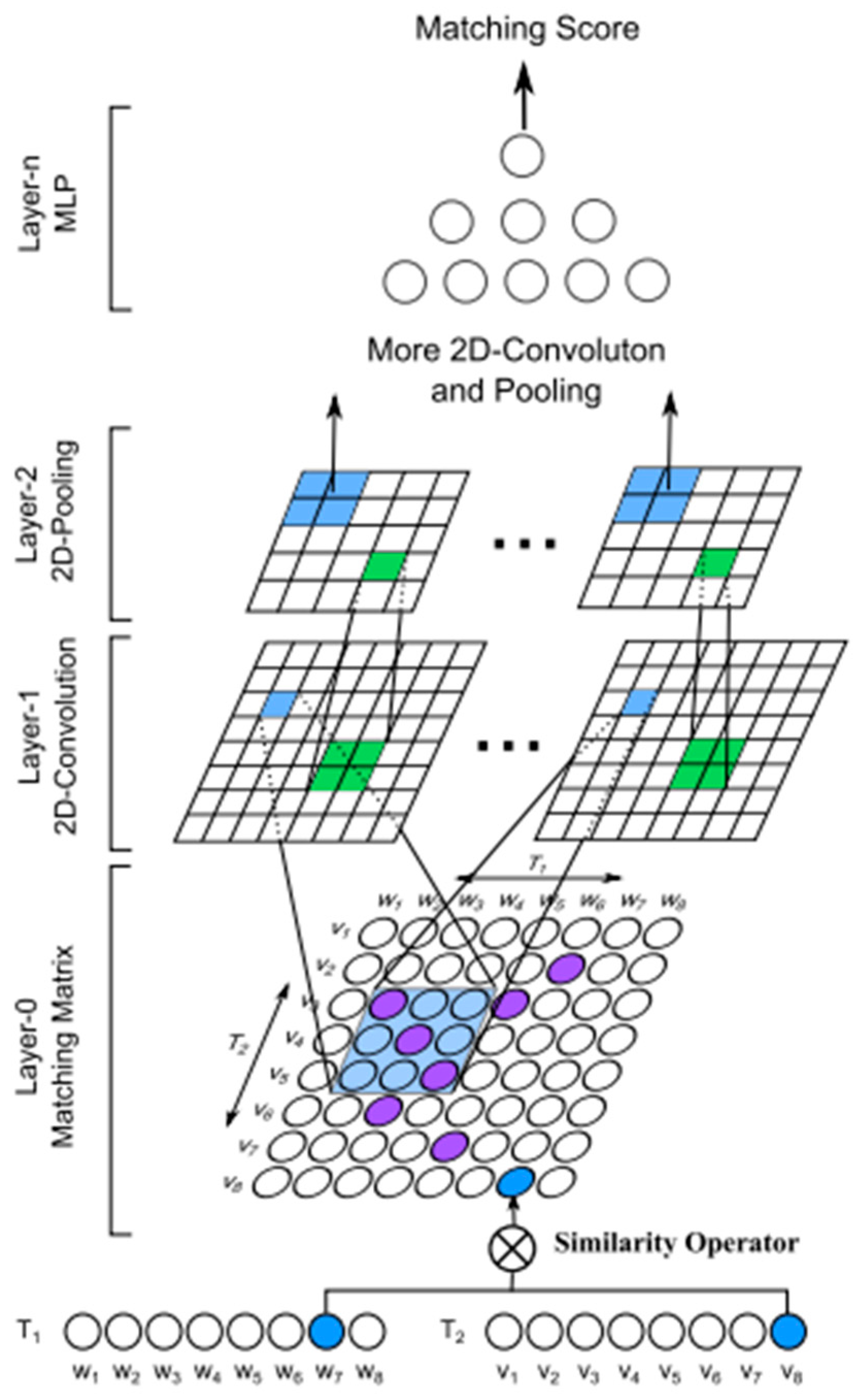
Inspired by CNN in image recognition (edge, corner, and other features can be extracted), the text is first calculated by similarity to construct a similarity matrix, and then convolution to extract features. Text matching is processed into image recognition [52]. MatchPyramid is illustrated in Figure 7.

Firstly, the MatchPyramid model uses the spatial position of the words in two sentences to construct the matching matrix. The matching matrix contains all the finest matching information. After that, the model regards the matching problem as an image recognition problem on this two-dimensional matching matrix.

Then, the matching matrix is extracted by using two-layer CNN, and the dynamic pool is used in the first layer CNN. Finally, the result of CNN is transformed by two-layer full connection that activated by sigmoid. Finally, the classification probability is calculated by SoftMax function.

The disadvantage of the model is that the network is complex, the resource consumption of model training is large, and a large number of supervised text matching data training is needed [53].

3.4. Based on Graph Structure

Recently, graphs as a form of structured text data have drawn great research attention from both academia and industry. The advantage of graph-based representation and calculation of text similarity lies in that the links between nodes are established through the edges of graph structures, so as to better judge the degree of similarity between nodes. According to the different types of graphs, they are mainly based on knowledge graph representation and graph neural network representation.

3.4.1. Knowledge Graph

Knowledge-graph representation learning is used to project the entities and relationships in the knowledge graph into a continuous low-dimensional vector space through machine learning technology, while maintaining the basic structure and properties of the original knowledge graph [54]. This has two advantages for text similarity: One is that the numerical calculation can be carried out directly in the continuous vector space, which is convenient to expand the calculation of similarity. The other lies in that the low-dimensional continuous knowledge graph vector representation is obtained by machine-learning technology. Furthermore, its learning process takes into account both local and global features of the knowledge graph. The generated entity and relation vector is essentially a more semantic representation, which can express semantic information efficiently [55].

The initial text can be regarded as a query graph, coordinating in the vector space, and are calculated by using translation mechanisms and other representation learning operators based on the query graph [56]. Then, the approximate results are found through the nearest search. By representing both the query and the answer (triple) as a vector, the semantic retrieval problem of the knowledge base is transformed into the problem of solving vector similarity [57].

3.4.2. Graph Neural Network

When there are many levels of data and connections, it is necessary to use the model to express the hierarchical relationship of the data and then derive the graph neural network (GNNs) [58,59].

The graph neural network (GNNs) is a connectionism model, which captures the dependency of the graph through the message transmission between the nodes of the graph [60]. Unlike the standard neural network, the graph neural network retains a state that can represent information of any depth from its neighborhood [61].

4. Discussion

The purpose of the current study was to make an overview of the development of text similarity measurement methods. It explains the similarity measurement methods from the combination of representation learning and distance calculation. These findings have significant implications for the understanding of how to represent text vectors. From the point of view of representation learning, the methods of character-based, semantic-based, neural network, and graph-based representation are described; from the point of view of distance calculation, the methods of spatial distance, angular distance, and Word Mover’s Distance (WMD) are described. Last, the classical and new algorithms are also systematically expounded and compared.

Taken together, these results suggest that there is an association between text distance and text representation. The text representation method provides a good basis for the calculation of text similarity.

The calculation of similarity based on string is simple and easy to implement. Apart from this, it can also have good results for some text with good performance through character-level comparison. For example, the winner’s system in the SemEval2014 sentence similarity task adopts the scheme of using vocabulary alignment [62]. However, the deficiency is that for two texts whose sentence meanings are very similar, the similarity calculated based on strings can capture neither the semantic similarity of the two texts nor the lexical semantics of the two texts.

The similarity calculation based on corpus takes into account the semantic information on the basis of strings, but there are still problems in dealing with the similarity of different terms in similar contexts [34]. Therefore, single-semantic text matching and multi-semantic text matching are considered to mine the deeper features of the text. Taking into account the multilevel structure of the text, through the way of graph representation, to mine the characteristics of the text, and then measure the similarity [63].

There are still many unanswered questions about text similarity, it includes the similarity representation method applied to the task. In future investigations, it might be possible to use a different text representation in which to express text semantics more richly.

5. Conclusions

Measuring the semantic similarity between two text fragments has been one of the most challenging tasks in natural language processing. Various methods have been proposed to measure semantic similarity over the years. This survey discusses the pros and cons of each approach. String-based methods take into consideration the actual meaning of text; however, they are not adaptable across different domains and languages. Corpus-based methods have a statistical background and can be implemented across languages, but they do not take into consideration the actual meaning of the text. Methods based on semantic text matching have good performance, but they require high computational resources and lack interpretability. Graph-structure methods need to rely on learning good graph representation to have good performance. It is clear from the survey that each method has its advantages and disadvantages, and it is difficult to choose one best model; however, most popular methods-based text representation and appropriate text distance have shown promising results over other independent models. This survey will provide a good foundation for researchers to find a new method to measure semantic similarity.

References

- Lin, D. An information-theoretic definition of similarity. In Proceedings of the International Conference on Machine Learning, Madison, WI, USA, 24–27 July 1998; pp. 296–304. [Google Scholar]
- Li, H.; Xu, J. Semantic matching in search. Found. Trends Inf. Retr. 2014, 7, 343–469. [Google Scholar] [CrossRef] [Green Version]
- Jiang, N.; de Marneffe, M.C. Do you know that Florence is packed with visitors? Evaluating state-of-the-art models of speaker commitment. In Proceedings of the 57th Annual Meeting of the Association for Computational Linguistics, Florence, Italy, 28 July–2 August 2019; pp. 4208–4213. [Google Scholar]
- Wang, Q.; Li, B.; Xiao, T.; Zhu, J.; Li, C.; Wong, D.F.; Chao, L.S. Learning deep transformer models for machine translation. arXiv 2019, arXiv:1906.01787. [Google Scholar]
- Serban, I.V.; Sordoni, A.; Bengio, Y.; Courville, A.; Pineau, J. Building end-to-end dialogue systems using generative hierarchical neural network models. In Proceedings of the Thirtieth AAAI Conference on Artificial Intelligence, Phoenix, AZ, USA, 12–17 February 2016. [Google Scholar]
- Pham, H.; Luong, M.T.; Manning, C.D. Learning distributed representations for multilingual text sequences. In Proceedings of the 1st Workshop on Vector Space Modeling for Natural Language Processing, Denver, CO, USA, 5 June 2015; pp. 88–94. [Google Scholar]
- Gomaa, W.H.; Fahmy, A.A. A survey of text similarity approaches. Int. J. Comput. Appl. 2013, 68, 13–18. [Google Scholar]
- Deza, M.M.; Deza, E. Encyclopedia of distances. In Encyclopedia of Distances; Springer: Berlin/Heidelberg, Germany, 2009; pp. 1–583. [Google Scholar]
- Norouzi, M.; Fleet, D.J.; Salakhutdinov, R.R. Hamming distance metric learning. In Proceedings of the Advances in Neural Information Processing Systems, Lake Tahoe, NV, USA, 3–6 December 2012; pp. 1061–1069. [Google Scholar]
- Manning, C.D.; Manning, C.D.; Schütze, H. Foundations of Statistical Natural Language Processing; MIT Press: Cambridge, MA, USA, 1999. [Google Scholar]
- Nielsen, F. A family of statistical symmetric divergences based on Jensen’s inequality. arXiv 2010, arXiv:1009.4004. [Google Scholar]
- Kullback, S.; Leibler, R.A. On information and sufficiency. Ann. Math. Stat. 1951, 22, 79–86. [Google Scholar] [CrossRef]
- Weng, L. From GAN to WGAN. arXiv 2019, arXiv:1904.08994. [Google Scholar]
- Vallender, S. Calculation of the Wasserstein distance between probability distributions on the line. Theory Probab. Appl. 1974, 18, 784–786. [Google Scholar] [CrossRef]
- Kusner, M.; Sun, Y.; Kolkin, N.; Weinberger, K. From word embeddings to document distances. In Proceedings of the International Conference on Machine Learning, Lille, France, 6–11 July 2015; pp. 957–966. [Google Scholar]
- Andoni, A.; Indyk, P.; Krauthgamer, R. Earth mover distance over high-dimensional spaces. In Proceedings of the Symposium on Discrete Algorithms, San Francisco, CA, USA, 20–22 January 2008; pp. 343–352. [Google Scholar]
- Wu, L.; Yen, I.E.; Xu, K.; Xu, F.; Balakrishnan, A.; Chen, P.Y.; Ravikumar, P.; Witbrock, M.J. Word mover’s embedding: From word2vec to document embedding. arXiv 2018, arXiv:1811.01713. [Google Scholar]
- De Maesschalck, R.; Jouan-Rimbaud, D.; Massart, D.L. The mahalanobis distance. Chemom. Intell. Lab. Syst. 2000, 50, 1–18. [Google Scholar] [CrossRef]
- Huang, G.; Guo, C.; Kusner, M.J.; Sun, Y.; Sha, F.; Weinberger, K.Q. Supervised word mover’s distance. In Proceedings of the Advances in Neural Information Processing Systems, Barcelona, Spain, 5–10 December 2016; pp. 4862–4870. [Google Scholar]
- Hunt, J.W.; Szymanski, T.G. A fast algorithm for computing longest common subsequences. Commun. ACM 1977, 20, 350–353. [Google Scholar] [CrossRef]
- Tsai, Y.T. The constrained longest common subsequence problem. Inf. Process. Lett. 2003, 88, 173–176. [Google Scholar] [CrossRef]
- Iliopoulos, C.S.; Rahman, M.S. New efficient algorithms for the LCS and constrained LCS problems. Inf. Process. Lett. 2008, 106, 13–18. [Google Scholar] [CrossRef]
- Irving, R.W.; Fraser, C.B. Two algorithms for the longest common subsequence of three (or more) strings. In Proceedings of the Annual Symposium on Combinatorial Pattern Matching, Tucson, AZ, USA, 29 April–1 May 1992; pp. 214–229. [Google Scholar]
- Levenshtein, V.I. Binary codes capable of correcting deletions, insertions, and reversals. Sov. Phys. Dokl. 1966, 10, 707–710. [Google Scholar]
- Damerau, F.J. A technique for computer detection and correction of spelling errors. Commun. ACM 1964, 7, 171–176. [Google Scholar] [CrossRef]
- Winkler, W.E. String Comparator Metrics and Enhanced Decision Rules in the Fellegi-Sunter Model of Record Linkage. 1990. Available online: https://files.eric.ed.gov/fulltext/ED325505.pdf (accessed on 31 August 2020).
- Dice, L.R. Measures of the amount of ecologic association between species. Ecology 1945, 26, 297–302. [Google Scholar] [CrossRef]
- Jaccard, P. The distribution of the flora in the alpine zone. 1. New Phytol. 1912, 11, 37–50. [Google Scholar] [CrossRef]
- Wang, S.; Manning, C.D. Baselines and bigrams: Simple, good sentiment and topic classification. In Proceedings of the 50th Annual Meeting of the Association for Computational Linguistics: Short Papers, Jeju Island, Korea, 8–14 July 2012; Volume 2, pp. 90–94. [Google Scholar]
- Salton, G.; Buckley, C. Term-weighting approaches in automatic text retrieval. Inf. Process. Manag. 1988, 24, 513–523. [Google Scholar] [CrossRef] [Green Version]
- Robertson, S.E.; Walker, S. Some simple effective approximations to the 2-poisson model for probabilistic weighted retrieval. In Proceedings of the International ACM Sigir Conference on Research and Development in Information Retrieval SIGIR’94, Dublin, Ireland, 3–6 July 1994; pp. 232–241. [Google Scholar]
- Rong, X. word2vec parameter learning explained. arXiv 2014, arXiv:1411.2738. [Google Scholar]
- Le, Q.; Mikolov, T. Distributed representations of sentences and documents. In Proceedings of the International Conference on Machine Learning, Bejing, China, 22–24 June 2014; pp. 1188–1196. [Google Scholar]
- Mikolov, T.; Chen, K.; Corrado, G.; Dean, J. Efficient estimation of word representations in vector space. arXiv 2013, arXiv:1301.3781. [Google Scholar]
- Pennington, J.; Socher, R.; Manning, C.D. Glove: Global vectors for word representation. In Proceedings of the 2014 Conference on Empirical Methods in Natural Language Processing (EMNLP), Doha, Qatar, 25–29 October 2014; pp. 1532–1543. [Google Scholar]
- Devlin, J.; Chang, M.W.; Lee, K.; Toutanova, K. Bert: Pre-training of deep bidirectional transformers for language understanding. arXiv 2018, arXiv:1810.04805. [Google Scholar]
- Deerwester, S.; Dumais, S.T.; Furnas, G.W.; Landauer, T.K.; Harshman, R. Indexing by latent semantic analysis. J. Am. Soc. Inf. Sci. 1990, 41, 391–407. [Google Scholar] [CrossRef]
- Kontostathis, A.; Pottenger, W.M. A framework for understanding Latent Semantic Indexing (LSI) performance. Inf. Process. Manag. 2006, 42, 56–73. [Google Scholar] [CrossRef]
- Landauer, T.K.; Dumais, S.T. A solution to Plato’s problem: The latent semantic analysis theory of acquisition, induction, and representation of knowledge. Psychol. Rev. 1997, 104, 211. [Google Scholar] [CrossRef]
- Landauer, T.K.; Foltz, P.W.; Laham, D. An introduction to latent semantic analysis. Discourse Process. 1998, 25, 259–284. [Google Scholar] [CrossRef]
- Grossman, D.A.; Frieder, O. Information Retrieval: Algorithms and Heuristics; Springer Science & Business Media: Berlin/Heidelberg, Germany, 2012; Volume 15. [Google Scholar]
- Hofmann, T. Probabilistic latent semantic analysis. arXiv 2013, arXiv:1301.6705. [Google Scholar]
- Blei, D.M.; Ng, A.Y.; Jordan, M.I. Latent dirichlet allocation. J. Mach. Learn. Res. 2003, 3, 993–1022. [Google Scholar]
- Wei, X.; Croft, W.B. LDA-based document models for ad-hoc retrieval. In Proceedings of the 29th Annual International ACM SIGIR Conference on Research and Development in Information Retrieval, Seattle, WA, USA, 6–11 August 2016; pp. 178–185. [Google Scholar]
- Sahami, M.; Heilman, T.D. A web-based kernel function for measuring the similarity of short text snippets. In Proceedings of the 15th International Conference on World Wide Web, Edinburgh, Scotland, UK, 23–26 May 2006; pp. 377–386. [Google Scholar]
- Li, Q.; Wang, B.; Melucci, M. CNM: An Interpretable Complex-valued Network for Matching. arXiv 2019, arXiv:1904.05298. [Google Scholar]
- Shen, Y.; He, X.; Gao, J.; Deng, L.; Mesnil, G. A latent semantic model with convolutional-pooling structure for information retrieval. In Proceedings of the 23rd ACM International Conference on Information and Knowledge Management, Shanghai, China, 3–7 November 2014; pp. 101–110. [Google Scholar]
- Huang, P.S.; He, X.; Gao, J.; Deng, L.; Acero, A.; Heck, L. Learning deep structured semantic models for web search using clickthrough data. In Proceedings of the 22nd ACM International Conference on Information & Knowledge Management, Burlingame, CA, USA, 27 October–1 November 2013; pp. 2333–2338. [Google Scholar]
- Sak, H.; Senior, A.; Beaufays, F. Long short-term memory based recurrent neural network architectures for large vocabulary speech recognition. arXiv 2014, arXiv:1402.1128. [Google Scholar]
- Hu, B.; Lu, Z.; Li, H.; Chen, Q. Convolutional neural network architectures for matching natural language sentences. In Proceedings of the Advances in Neural Information Processing Systems, Montreal, QC, Canada, 8–13 December 2014; pp. 2042–2050. [Google Scholar]
- Wan, S.; Lan, Y.; Guo, J.; Xu, J.; Pang, L.; Cheng, X. A deep architecture for semantic matching with multiple positional sentence representations. In Proceedings of the Thirtieth AAAI Conference on Artificial Intelligence, Phoenix, AZ, USA, 12–17 February 2016. [Google Scholar]
- Pang, L.; Lan, Y.; Guo, J.; Xu, J.; Wan, S.; Cheng, X. Text matching as image recognition. In Proceedings of the Thirtieth AAAI Conference on Artificial Intelligence, Phoenix, AZ, USA, 12–17 February 2016. [Google Scholar]
- Liu, Z.; Xiong, C.; Sun, M.; Liu, Z. Entity-duet neural ranking: Understanding the role of knowledge graph semantics in neural information retrieval. arXiv 2018, arXiv:1805.07591. [Google Scholar]
- Chen, X.; Jia, S.; Xiang, Y. A review: Knowledge reasoning over knowledge graph. Expert Syst. Appl. 2020, 141, 112948. [Google Scholar] [CrossRef]
- Zhu, G.; Iglesias, C.A. Computing semantic similarity of concepts in knowledge graphs. IEEE Trans. Knowl. Data Eng. 2016, 29, 72–85. [Google Scholar] [CrossRef] [Green Version]
- Bordes, A.; Usunier, N.; Garcia-Duran, A.; Weston, J.; Yakhnenko, O. Translating embeddings for modeling multi-relational data. In Proceedings of the Advances in Neural Information Processing Systems, Lake Tahoe, NV, USA, 5–8 December 2013; pp. 2787–2795. [Google Scholar]
- Dong, L.; Wei, F.; Zhou, M.; Xu, K. Question answering over freebase with multi-column convolutional neural networks. In Proceedings of the 53rd Annual Meeting of the Association for Computational Linguistics and the 7th International Joint Conference on Natural Language Processing (Volume 1: Long Papers), Beijing, China, 26–31 July 2015; pp. 260–269. [Google Scholar]
- Gilmer, J.; Schoenholz, S.S.; Riley, P.F.; Vinyals, O.; Dahl, G.E. Neural message passing for quantum chemistry. In Proceedings of the 34th International Conference on Machine Learning, Sydney, Australia, 6–11 August 2017; Volume 70, pp. 1263–1272. [Google Scholar]
- Zhou, J.; Cui, G.; Zhang, Z.; Yang, C.; Liu, Z.; Wang, L.; Li, C.; Sun, M. Graph neural networks: A review of methods and applications. arXiv 2018, arXiv:1812.08434. [Google Scholar]
- Vashishth, S.; Yadati, N.; Talukdar, P. Graph-based Deep Learning in Natural Language Processing. In Proceedings of the 7th ACM IKDD CoDS and 25th COMAD, Hyderabad, India, 5–7 January 2020; pp. 371–372. [Google Scholar]
- Wu, Z.; Pan, S.; Chen, F.; Long, G.; Zhang, C.; Philip, S.Y. A comprehensive survey on graph neural networks. IEEE Trans. Neural Netw. Learn. Syst. 2020. [Google Scholar] [CrossRef] [PubMed] [Green Version]
- Sultan, M.A.; Bethard, S.; Sumner, T. Dls@ cu: Sentence similarity from word alignment and semantic vector composition. In Proceedings of the 9th International Workshop on Semantic Evaluation (SemEval 2015), Denver, CO, USA, 4–5 June 2015; pp. 148–153. [Google Scholar]
- Liu, B.; Guo, W.; Niu, D.; Wang, C.; Xu, S.; Lin, J.; Lai, K.; Xu, Y. A User-Centered Concept Mining System for Query and Document Understanding at Tencent. In Proceedings of the 25th ACM SIGKDD International Conference on Knowledge Discovery & Data Mining, Anchorage, AK, USA, 4–8 August 2019; pp. 1831–1841. [Google Scholar]
Figure 1.
Measurement of text similarity.
Figure 2.
Word2vec’s model architectures. The continuous bag of words (CBOW) architecture predicts the current word based on the context, and the skip-gram predicts surrounding words given the current word [34].
Figure 3.
Figure from <Bert: Pre-training of deep bidirectional transformers for language understanding>. BERT’s (bidirectional encoder representation from transformers) model architectures. BERT uses a bidirectional transformer. BERT’s representations are jointly conditioned on both the left and right context in all layers [36].
Figure 4.
Illustration of the deep-structured semantic models (DSSM). It uses a DNN (Deep Neural Networks) to map high-dimensional sparse text features into low-dimensional dense features in a semantic space [48].
Figure 5.
Architecture-I for matching two sentences [50].
Figure 6.
Illustration of multi-view bidirectional long and short-term memory (MV-LSTM) [51].
Figure 7.
An overview of MatchPyramid on text matching [52].
© 2020 by the authors. Licensee MDPI, Basel, Switzerland. This article is an open access article distributed under the terms and conditions of the Creative Commons Attribution (CC BY) license (http://creativecommons.org/licenses/by/4.0/).
Share and Cite
MDPI and ACS Style
Wang, J.; Dong, Y. Measurement of Text Similarity: A Survey. Information 2020, 11, 421. https://0-doi-org.brum.beds.ac.uk/10.3390/info11090421
AMA Style
Wang J, Dong Y. Measurement of Text Similarity: A Survey. Information. 2020; 11(9):421. https://0-doi-org.brum.beds.ac.uk/10.3390/info11090421
Chicago/Turabian StyleWang, Jiapeng, and Yihong Dong. 2020. "Measurement of Text Similarity: A Survey" Information 11, no. 9: 421. https://0-doi-org.brum.beds.ac.uk/10.3390/info11090421
Note that from the first issue of 2016, this journal uses article numbers instead of page numbers. See further details here.