2. Affective Multimedia Databases: Definition, Architecture and Usage
Affective picture databases are most frequently employed in the controlled stimulation of emotional reactions for experimentation in cognitive sciences, psychology, neuroscience, and different interdisciplinary studies, such as human–computer interaction (HCI) [
9,
10,
11]. Simply put, they are experts’ tools designed for intentionally provoking targeted emotional reactions in exposed subjects. They have many practical uses related to research in perception, memory, attention, reasoning, and, of course, emotion. Many such databases have so far been developed. The most popular ones, which are free for use by researchers, are: the International Affective Picture System (IAPS) [
9,
10], the Nencki Affective Picture System (NAPS) [
12] (with its extensions NAPS Basic Emotions [
13] and NAPS Erotic Subset [
14]), the Geneva Affective Picture Database (GAPED) [
15], the Open Library of Affective Foods (OLAF) [
16], the DIsgust-RelaTed-Images (DIRTI) [
17], the Set of Fear-Inducing Pictures (SFIP) [
18], the Open Affective Standardized Image Set (OASIS) [
19], and the most recent one, the Children-Rated Subset to the NAPS [
20]. In addition, a recent list of affective picture databases with different emotionally-annotated multimedia formats and exemplars of the research conducted with these database is available in [
8]. An example of affective pictures from the OASIS database, with semantic tags included, is shown in
Figure 2. The OASIS employs similar emotional and semantic models to the IAPS database.
New affective databases for provoking emotional responses are being continuously developed. This trend is encouraged by the growth in the variety and complexity of, and in demands for intensity and precision in, the experimentation by the researchers. Although they are invaluable tools in their field of practice, the affective multimedia databases have two important drawbacks that can be at least alleviated, if not completely eliminated, by utilizing methods from computer science and information retrieval. These drawbacks are demanding and time-consuming construction and retrieval of affective multimedia documents. Both are related to inefficient search of the databases, which is caused by their rudimentary and inadequate semantic representation model.
It is hard to define a specific unitary structure of affective multimedia databases, since there is no accepted standard for their construction. However, although they are different, some important common, distinctive features may be established [
8]. Most importantly, and in the context of this paper, document semantic annotations use a sparse bag-of-words model. In the affective databases, a single multimedia stimulus is tagged with an unsupervised glossary. Frequently, a document is tagged with a single free-text keyword, and different tags are used to describe the same concept. For example, a picture showing an attack dog in the IAPS database could be tagged as “dog”, “attack”, “AttackDog”, or “attack_dog”, etc. Synonym tags such as “canine” or “hound” are also used. Furthermore, semantic relations between different concepts are undefined. The lexicon itself does not implement semantic similarity measures and there are no criteria to estimate relatedness between concepts. For example, in such a model, it is difficult to determine that “dog” and “giraffe” are closer to each other than “dog” and “door”. This is a huge flaw in the document retrieval process because a search query must match the keywords only lexically. In this setting, a more semantically meaningful interpretation of the query and annotating tags is not possible. The inadequate semantic descriptors result in three negative effects that impair information retrieval: (1) low recall, (2) low precision and high recall, or (3) vocabulary mismatch. Moreover, affective multimedia databases do not contain their own hierarchical model of semantic labels and do not reuse external knowledge bases.
Unlike semantics, the description of multimedia affect is much more efficient and standardized across the currently published affective multimedia databases. The two most common models of emotion are the pleasure-arousal-dominance (PAD) dimensional [
21] and discrete models [
22].
3. Overview of Concept-Based Image Retrieval with Boolean Classification
In concept-based, also known as description-based or text-based, image retrieval, binary or binomial classification is an essential step in the selection of true results [
25]. In this process, lift charts can be used in two different ways: (1) to determine the cutoff rank of retrieved items, and (2) to assess the quality of the retrieval itself.
In concept-based document retrieval systems, as well as in image retrieval systems as their subtype, a new search is started by entering a query that constraints the items that should be retrieved. The query must be translated into the set of concepts that represents a set of documents being searched for adequately well [
1,
2]. The formality and expressivity of the concept set depend on the chosen knowledge representation model. Transformation of text to concepts may be trivial in the case where it is performed as a series of search tags or keywords. The search may greatly benefit if an underlying knowledge base is used that defines concept labels, their properties, and relationships between them [
7].
In the next step, the query concepts must be brought into a functional relationship and quantitatively compared with descriptions of images stored in the multimedia repository. With a technique called “query by example”, the concepts are not entered directly, but fetched from a description of an archetypical image, which was uploaded into the system instead of the query [
7]. In text-based systems, describing concepts must be provided together with the example image itself. This is usually accomplished by letting users choose one or more similar images already in the repository [
1,
2].
After a search query has been entered, in the next step of the retrieval process, each concept in the search text is compared to every concept
in descriptions of images stored in the repository. A suitable measure is then used to rank images according to their relatedness or similarity to the search query. The similarity measure is a function
, which takes two concepts from the set of all concepts
as its domain and provides a real number in a closed interval between 0.0 and 1.0 as a measure of closeness between the two concepts
and
Similarity measures between pairs of concepts in the query
and image description
are combined with an aggregation function. The aggregation may be any suitable function, but usually it is a sum or product of individual similarity assessments [
26]. If items in the repository are described with labels from a knowledge base, then it is possible to use concept distance measures, which are more formal and semantically more meaningful than lexical measures. Examples of both sets of measures can be found in [
1,
2]. Apart from the expressiveness of image description, the choice of the similarity and aggregation functions is crucial for the quality of the retrieval.
The results, i.e., retrieved documents, are represented as an ordered list
…,
Each image is assigned with a rank
which is the sequence number of the image in the returned list. Consequently, if
items are being returned, the first item
has the rank
the second one
and the rank of the last item
is
For a search to be considered successful, documents closer to the posed query should appear first, i.e., near the beginning of the returned results, and conversely, less related documents should appear more towards the end of the list. In other words, items more relevant to the query have a lower rank and those less relevant have a higher rank number. Ideally, the similarity of items in the returned list should be a monotonically decreasing and continuous function. As users browse through the list, from the first document towards the last, they expect their relevancy to continuously decrease. It would be counterintuitive and indeed harmful if items being sought are located at the end of the list. Such items may be unintentionally overlooked. Therefore, in an ideal series Equation (3) is valid:
where
is the similarity of item
If a large number of documents are stored in the repository, it would be costly to retrieve all of them at once. In such circumstances, only the best documents should be presented, while others are disregarded. The decision boundary is set at a rank cutoff
where items
will be displayed to users and
will not. Preferably, the cutoff value must be chosen so that precision and recall are maximized in order to display as many relevant documents in the repository as possible. Finally, after the documents have been classified and ranked, they may be extracted from the repository with their textual descriptions and presented to the user in the specific order consistent with their appointed rank.
4. Binary Classification with Lift Charts
Lift charts are a type of charts, such as the receiver operating characteristic (ROC) curves and precision-recall curves, which are often utilized in machine learning for visualization and evaluation of classification models. They can be especially useful in cases where the number of false positive observations is unavailable and, subsequently, more common machine learning evaluation methods, such as the ROC curves, cannot be constructed. Lift charts are primarily used as a tool for observing the improvement that a classifier makes against a random guess. In previously published literature they are described in this respect [
3,
30,
31].
However, the second use of lift charts—which is in the focus of this paper—is in the binary classification of ranked results. In this application, lift charts can be optimized to increase retrieval precision or recall. The difference in optimization is achieved with the choice of rank cutoff. In optimization for precision, the cutoff is commonly set to a lower rank, while if classification is adjusted for recall (i.e., better sensitivity), the cutoff is set at a higher rank. The exact choice of rank depends on the data and the desired classification performance.
In the document retrieval experiment, the lift charts have been demonstrated to be a helpful method for binomial classification in situations where ground truth annotations are inadequate or unattainable and the precise rank of affective multimedia documents cannot be determined. Ground truth annotations or labels are very important in concept-based retrieval, as they represent the true description of documents. In fact, they specify an objective and complete knowledge about document content in description-based retrieval paradigms. The annotations can be represented by any adequately expressive model, such as keywords from supervised or controlled vocabularies as in the bag-of-words model [
1,
2]. Ground truth labels of images are always provided by a trusted authority. The labels are added either by a human domain expert or automatically by image analysis, depending on the complexity of the problem [
32]. However, in some information retrieval applications, the labels are not available or cannot be correctly defined. In such circumstances, both the true category and rank of retrieved results cannot be known accurately and, subsequently, the search performance deteriorates. In these cases, the capability to assign documents to the correct class becomes more important than the effectiveness of finding the correct document rank [
1,
2]. The rationale is that if the rank is incorrect and document order in the results list is inaccurate, at least they will be correctly classified and presented to a user. In other words, it is better to retrieve a correct document albeit with an incorrect position in the results list, than to not retrieve it at all. The lift charts can assist in improving precision and recall in such settings.
It should be noted that the term “profit charts” is sometimes used in the literature instead of “lift charts” (for example in [
33]). However, the two are not completely identical. A profit chart contains the same information as a lift chart, but also presents the estimated increase in profit that is related to a specific model [
3].
Formally, in document retrieval, a lift chart is a two-dimensional (2D) graph with its
x-axis representing the ranked number of results and its
y-axis showing the true positive (
measure. Such a lift chart may be defined as in Equation (8):
where
is the total number of documents being classified,
is the ranked document’s ordinal number, and
is the true positive value at position
.
However, for better convenience, relative ratios are often used for the definition of chart axes instead of total numbers. In this approach, the
x-axis represents the proportion of ranked results (%) and the
y-axis represents the true positive rate (
, which is the ratio of correctly classified instances and total number of documents in the retrieved set, as was explained in
Section 3.1. Consequently, the lift chart function can be defined as in Equation (9):
where
represents the proportion of the result and
is the value of the true positive rate at ranked position
.
Therefore, a lift chart is created by calculating or for specific values of In practice, lift charts are not smooth but stepwise, i.e., each point on the graph defines a column (a step or an increment) with the point in its upper left corner. To facilitate and precipitate the plotting process, usually only representative values of are considered in discrete increments, such as each 5% (t/N = 0.0, 0.05, 0.1, …, 0.95, 1.0) or 10% (t/N = 0.0, 0.1, 0.2, …, 0.9, 1.0) data segments. The convex curve obtained by drawing the given points is called a lift chart. The coarseness of charts’ shapes is directly proportional to their increment size. Smaller steps, as the difference between two consecutive values of will have the effect of a smoother curve shape, while larger steps will produce wider discrete columns and a coarser or step-like hull. Note that the curve can be at most calculated for each classified item, which is not recommended if the retrieved set is very large.
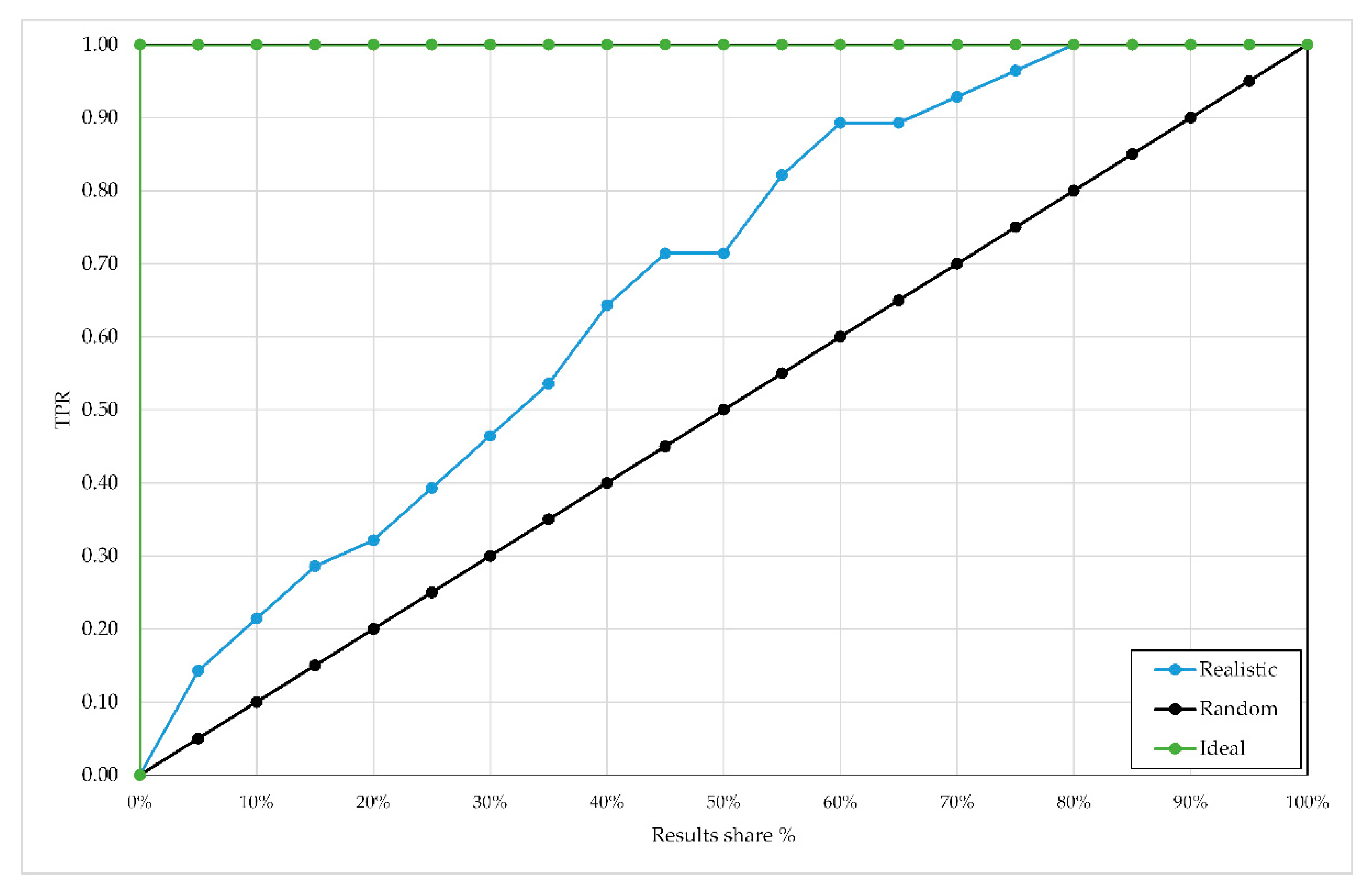
An ideal classifier model will have for because a perfect retrieval system will provide only TP documents to users, correctly disregarding TN, FN, and FP instances. The corresponding lift chart is a vertical line along the left edge and a horizontal line on the top edge of the plot area. On the other hand, the lift chart of a naïve classifier that categorizes documents just by random guessing is a straight diagonal line from the lower left to the upper right corner. Such a lift chart is defined by two points, and .
In binary settings, a random classifier classifies 50% of pictures to the “True” category and 50% to the “False” category. As such, it has the worst performance of all possible classifiers and is used as a preferable reference for the evaluation of machine learning models. Thus, it is commonly assumed that the performance of any actual classification model is better than the classification performed simply by chance and worse than that of an ideal classifier.
Three lift charts of a realistic classifier from the experiment in this paper, for ideal and random classifiers with an increase of 5% in
, are shown in
Figure 3.
The improvement of a model is evaluated in terms of a numerical measure called the lift score or, more commonly, the lift. By comparing the lift for all portions of a dataset and for different classifiers, it is possible to determine which model is better, or even optimal, and which percentage of the cases in the dataset would benefit from applying the model’s predictions. Classifiers may have similar or even identical performance for some values of making the lift negligible or very small, but, at the same time, their performance can be considerably different in other sections. Therefore, the lift must be determined for all steps to establish the maximum score.
Formally, the lift is a measure of predictive model effectiveness calculated as the ratio between the results obtained with and without the predictive model. The lift is commonly expressed in relative terms as a percentage where, for example, a lift of 100% implies a double improvement in predictiveness compared to a referent model, a lift of 200% a triple improvement, and so on.
The area under curve (AUC), or more precisely, the area under lift chart can be used as a measure of classification quality. Since, in practice, lift charts are not smooth, but stepwise, the sum of all discrete columns in a stepwise lift chart is equal to
Using integration, it can be easily shown, as in Equation (10), that the random classifier has an area under the curve equal to:
where
is area under the curve of the same classifier [
5]. It is defined in Equation (11):
The random classifier has and a perfect classifier has Therefore, the of actual classifiers lies between and Since always depends on the to ratio, if then it is possible to use the approximation Moreover, it should be noted that a random classifier has while a perfect classifier has . Classifiers used in practice should therefore be somewhere in between, and preferably have an close to the value of 1.
AUCs of the lift charts from
Figure 3 are portrayed in
Figure 4. In this case, with the relative proportion in the dataset on the
x-axis, numerical integration for the realistic classifier gives
. This is 1.3428 times more than for the random guess (
and 1.4894 times less than for a perfect classifier (
.
5. Evaluation of Affective Image Retrieval with Lift Charts as Binomial Classifiers in Ranking
In the experiment, binomial classification of images was evaluated with lift charts to provide a real-life example and indicate benefits and drawbacks of their utilization in image retrieval. The experiment demonstrated the application of lift charts as explained in
Section 4. For this, a dataset
consisting of
N = 800 pictures was taken from the IAPS corpora [
9,
10]. This database was chosen because it is the most frequently utilized one, and also one of the largest affective multimedia databases [
8]. Moreover, its architecture may be considered typical for this type of datasets. Other repositories have comparable semantic models with unsupervised annotation glossaries and sparse tagging. The selected pictures are visually unambiguous with easily comprehensible content. The content of each picture was described with one keyword
from an unsupervised glossary
The glossary contained 387 different keywords. The set of all queries
applied in the evaluation consisted of different keywords taken from the annotation glossary (
). For every query
a subset of documents
with
= 100 pictures was randomly preselected and then classified using lexical relatedness measures [
34]. Each subset
was queried three times: with one, two, or three different words. Only the terms from
were used as queries, which guaranteed that the retrieved sets were nonempty. The setup for the experiment was reused from a previous research [
34] but with the expanded dataset
, which also resulted in a different glossary
queries
and assortment of all preselected subsets
. Compared to [
35], the additional images in the dataset provide greater credibility in the results of this study.
Two lexical relatedness measures were used for ranking: naïve string matching and the Levenshtein distance (i.e., edit distance) [
34]. Each subset
was classified once for each relatedness algorithm, with rank cutoff independently optimized twice: first for precision and then for recall. The goal of classification for precision was to maximize the fraction of pictures relevant to posited queries. Classification for recall tried the opposite: to maximize the share of relevant pictures in
In practice, the two optimization methods are contradictory: the former results in high accuracy and a small number of retrieved samples, and the latter optimization returns a large share of samples, but with considerably lower accuracy.
5.2. Binomial Classification with Lift Charts
In the experiment, all queries
returned
images sorted in descending order according to the selected distance metric. It was essential to find the threshold value
t that fixes the boundary between categories, i.e., how the retrieved pictures will be classified. Given a picture
and its rank
in the retrieved results, where
indicates the most relevant picture
the picture
was assigned to the category
as in Equation (15):
Thus, in every query, the retrieved corpus was binarily classified into two subsets: (1) the category “True” with relevant pictures to the search query, and (2) the category “False” with irrelevant pictures. The threshold value (i.e., rank cutoff) was set individually for every query with a lift chart.
For the maximum precision, the cutoff was assigned to the rank with the highest lift factor. This adaptive approach assures a more objective ranking and better retrieval performance than a constant classification threshold. For example, if a result set has the maximum lift factor for rank to achieve the highest precision, only samples with should be classified as “True” and all others with as “False”.
This optimization approach contrasts with the fitting for recall (sensitivity), where the classification threshold is set to a relatively high value to include as many true positives as possible. In the experiment, the threshold was set at 90%. On the other hand, this approach will inevitably result in a lower precision, because many false positives will also be retrieved. It is important to point out that by using lift charts it is always possible to choose between higher precision or recall and customize the classification accordingly.
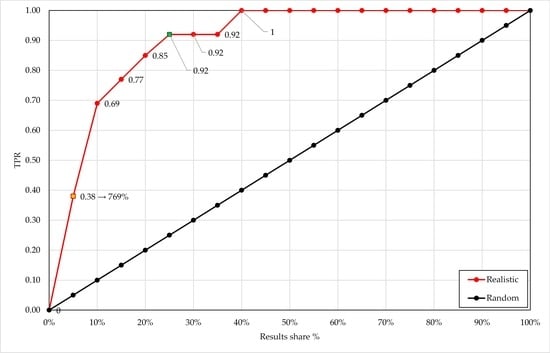
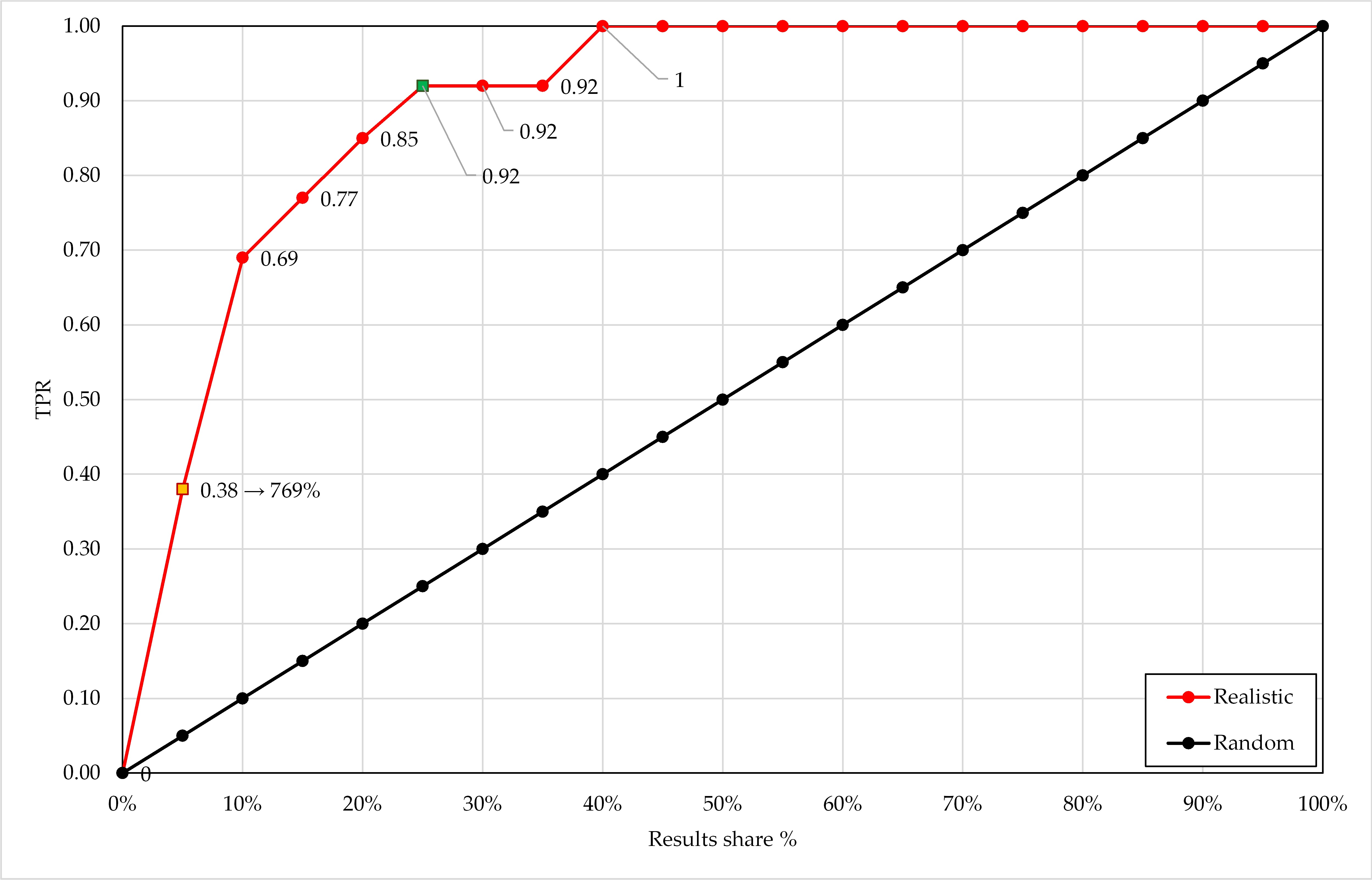
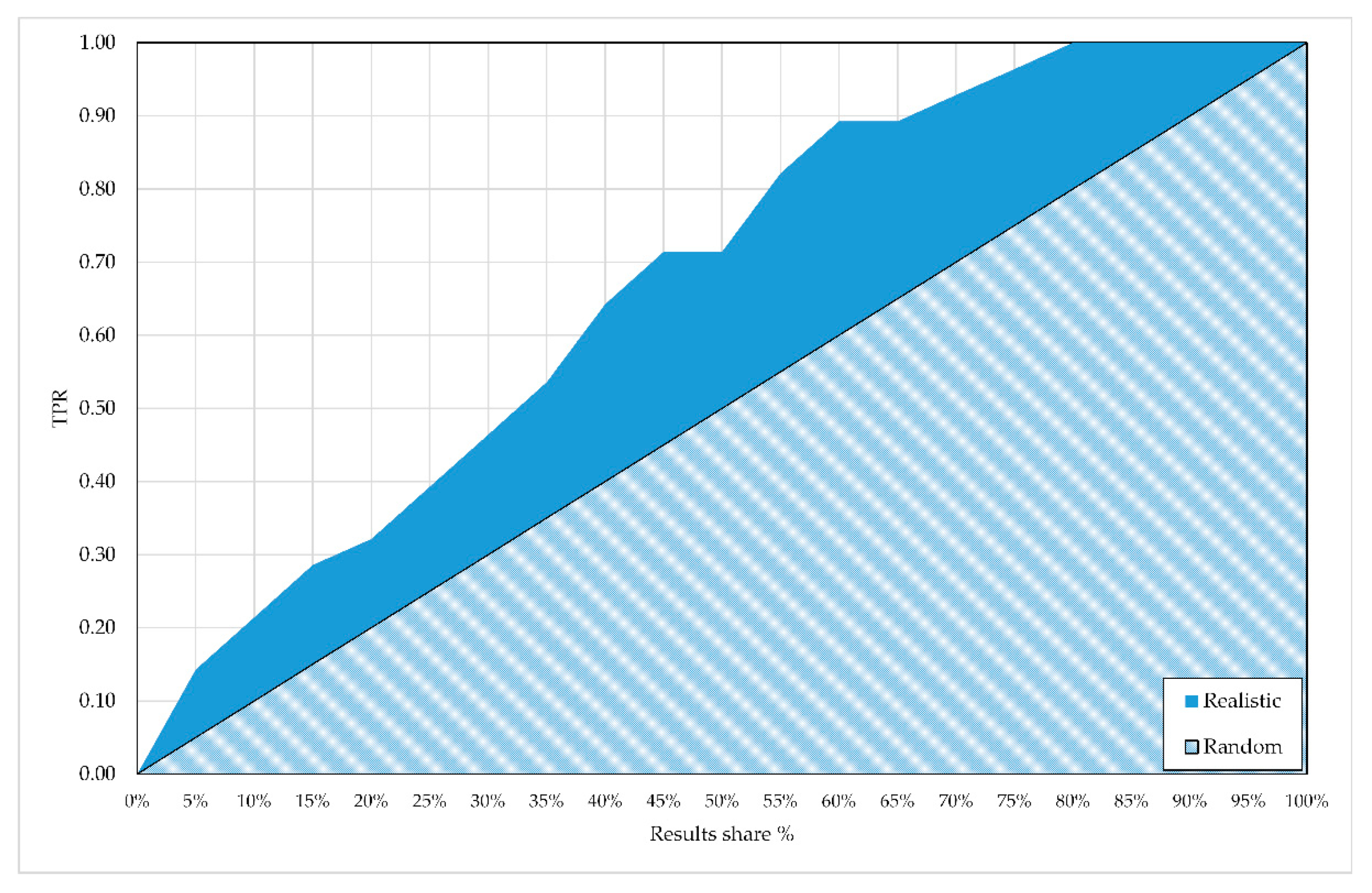
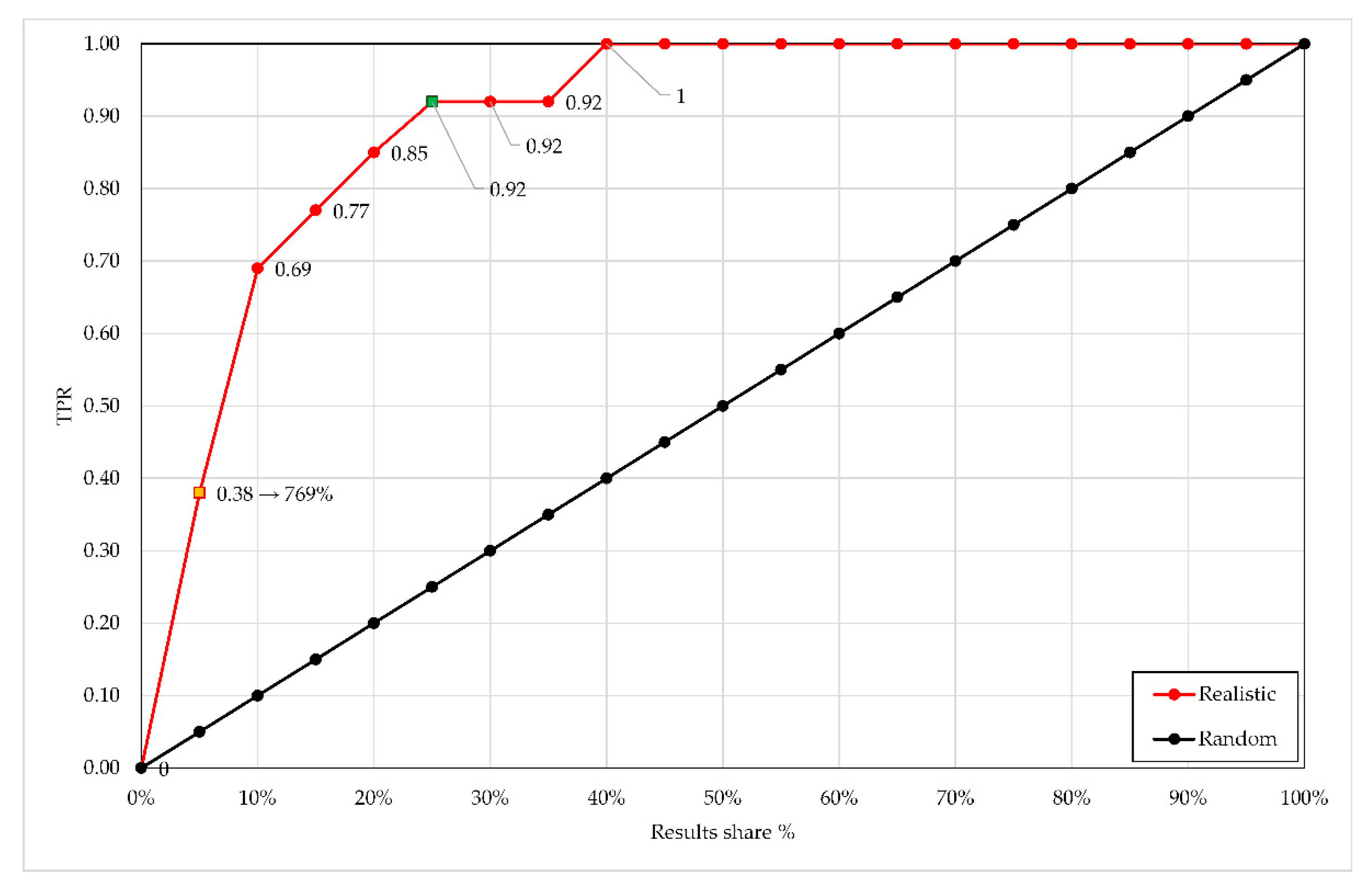
In the experiment, the classifications were optimized twice for both goals and the lift charts were split into 5% intervals. An example from the experiment is presented in
Figure 5 below. Here, the dataset was queried with a single keyword “man” and ranked using the Levenshtein algorithm.
In
Figure 5, the red curve represents the lift chart of the classifier used in the picture retrieval study and a random classifier is designated with the black line. The orange marker represents the maximum lift over a random classifier. As can be seen in
Figure 5, the maximum lift of 769% was achieved for
and
. All other data segments provided lower lifts.
Additionally, in
Figure 5, the green marker at 0.92 TPR represents the cutoff of optimization for recall because it indicates the lowest share of results (in this case 0.25 or 25%) where TPR ≥ 0.9. Thus, in this application for optimal recall, the cutoff must be set as
. Again, pictures with
will be presented as search results, and all other pictures with
will be omitted. The recall was increased, but in a trade-off, precision and accuracy were reduced.
In the experiment, ground truth annotations of images were available, but they were semantically inadequate to fully describe the pictures and their content. Subsequently, domain experts could not agree on the true rank of images and only the assignment into the two classes was possible. This kind of problem is especially suited for lift charts, as they can be used to quantitatively evaluate and compare different classifiers, even when document rank cannot be known.
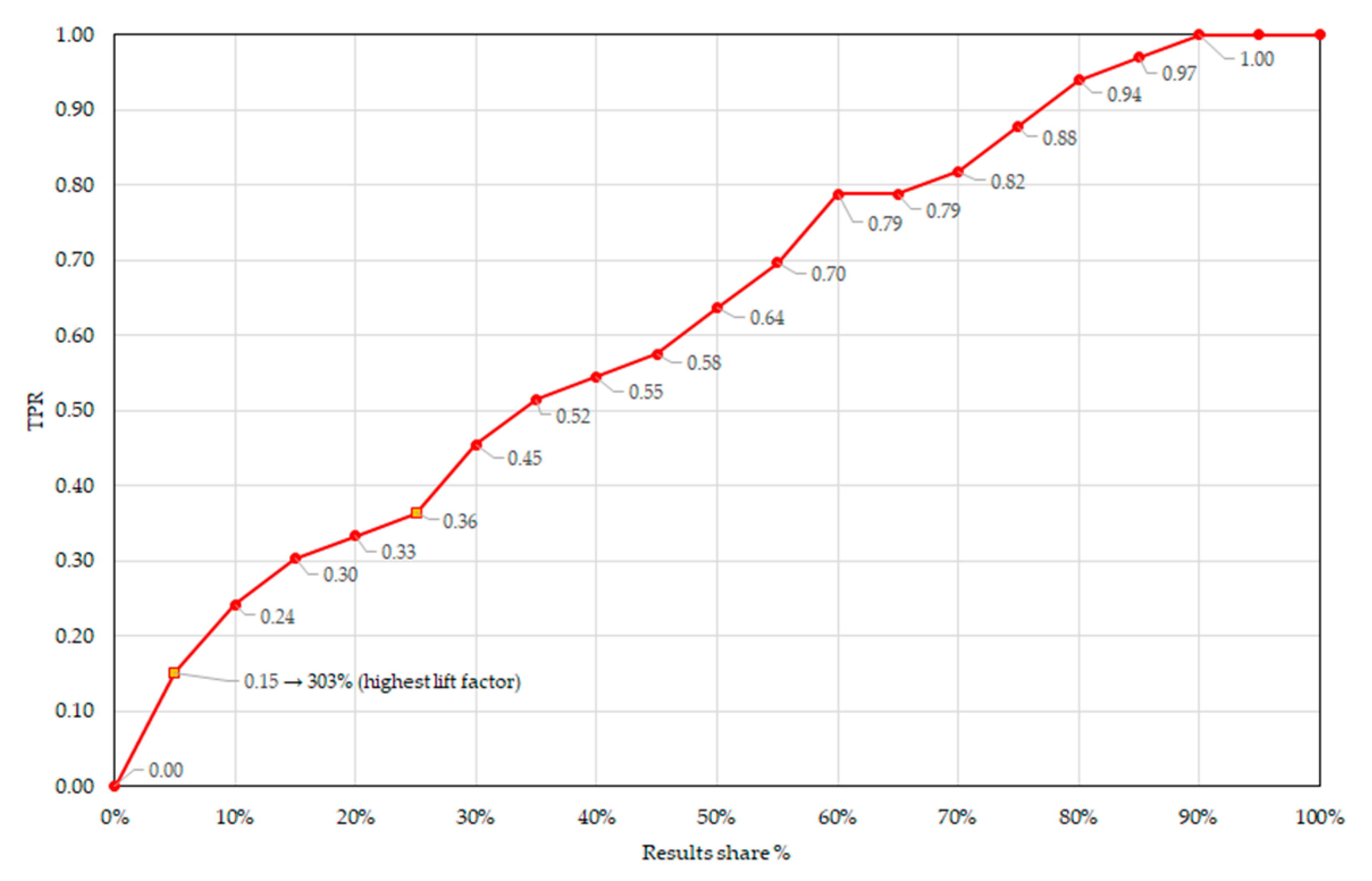
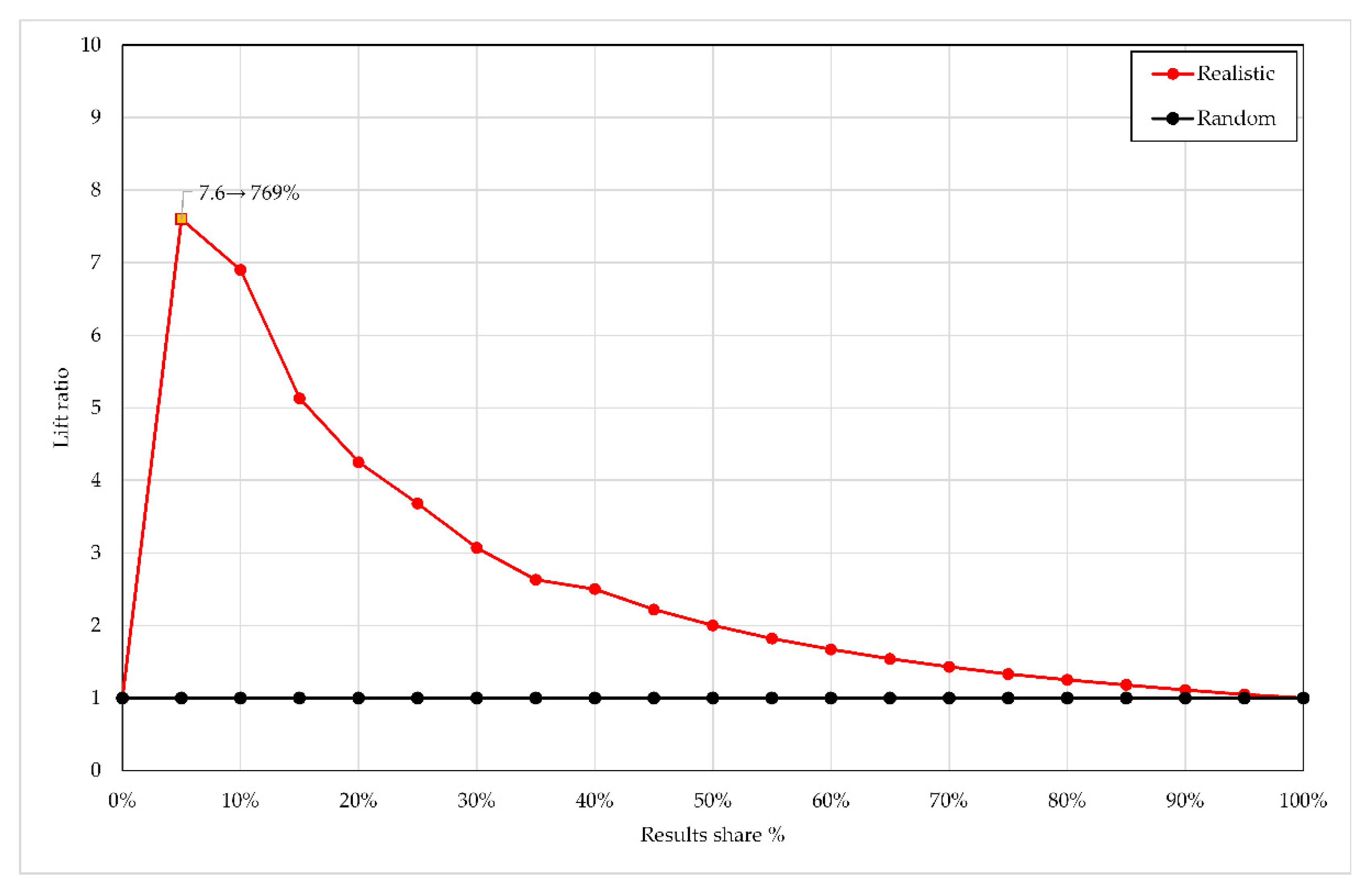
The detailed progress of the lift depending on the results share
is displayed in
Figure 6. Consequently, the 5% point must be chosen for cutoff in optimization for precision: pictures with rank
should be assigned to the class “
True” and displayed to users, and pictures with
to the class “
False“ and disregarded. With a cutoff at
,
or in other words, only 38% of the TP pictures in the set were retrieved. This contributes to poor performance in recall but improves precision and accuracy.
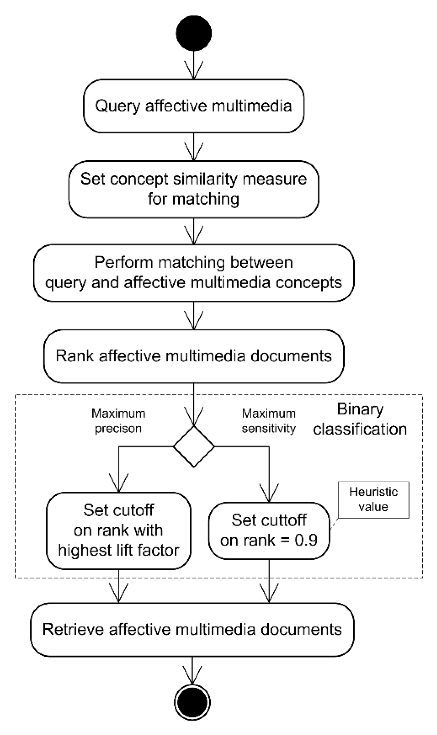
For better clarity, the entire affective multimedia retrieval process is displayed in the UML activity diagram in
Figure 7.
The affective multimedia retrieval starts with a user querying the affective multimedia database using an appropriate computer interface. The users enter free-text keywords as their query and select which concept similarity measure will be used for matching. The system calculates semantic similarity between the entered query and descriptions of multimedia in the database. This step could be time-consuming, depending on the computational complexity of the chosen similarity algorithm. The duration of the ranking also linearly depends on the size of the database. After ranking has finished, affective multimedia documents are sorted in the order proportional to the similarity of their describing concepts to the concepts in the posed query. Since documents are indexed, the sorting should be less complex than the ranking. In the next step, the binary classification using lift charts is performed. If the optimization for precision is desired, then the system will find the rank with the maximum lift factor and set the cutoff at that value. Alternatively, if the search must be optimized for recall while retaining the highest achievable level of precision, then the cutoff is set at a fixed rank of 0.9. All documents with a rank less than the cutoff value are classified as positive, and all others are classified as negative. The described binary classification of affective multimedia documents is a very important step and therefore has been explained in detail in this section. Finally, in the last step, the system will fetch all positively classified documents. All documents of positively classified instances are retrieved from the multimedia repository and presented to the user. This action may also be laborious and time-consuming, but its complexity hinges on the performance of storage and data transfer subsystems and on the processor, like the ranking.
6. Experiment Results
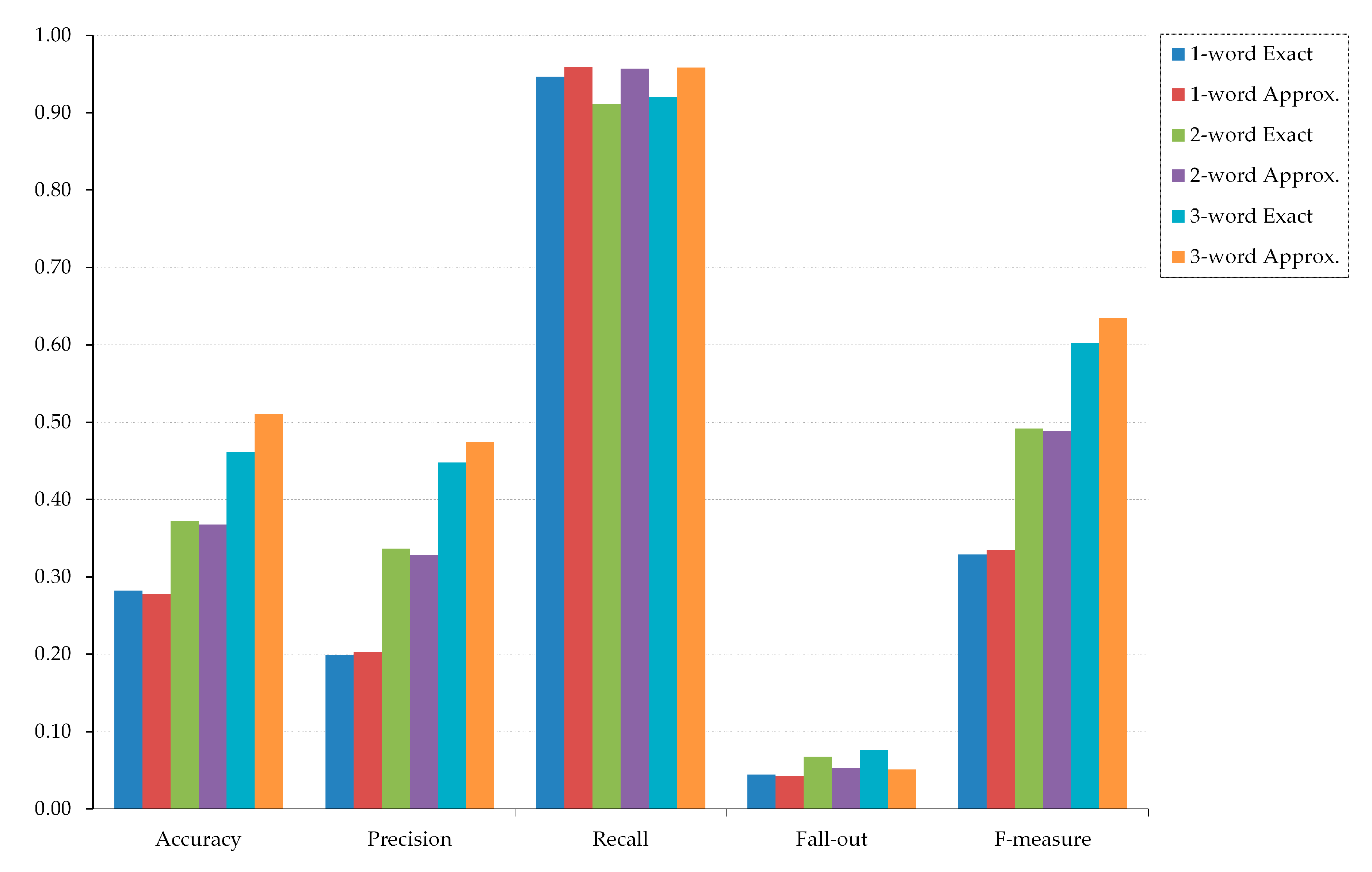
The aggregated retrieval results optimized for recall are shown in
Table 1, while those optimized for precision are shown in
Table 2. Each table presents five essential performance measures (accuracy, precision, recall, fall-out, and F-measure) for two lexical similarity algorithms (exact and approximate), which were used with one-, two-, and three-word queries. Furthermore, results from the tables are displayed as graphs in
Figure 8 and
Figure 9. The experiment in [
35] used a relatively similar portion of the IAPS dataset (62%) compared to this experiment (66.95%), which explains why some values obtained in these two experiments are identical. Statistically significant differences between exact and approximate lexical similarity algorithms are marked in
Table 1 and
Table 2. In
Table 3, we show the statistically significant differences between one-word, two-word, and three-word queries. Statistically insignificant differences are not depicted.
As can be seen from
Table 1 and
Figure 8, with classifications optimized for recall, where cutoff was set at 90% of TPR in the ranked results, multiword word queries performed better than single word queries in general: the performance of the three-word queries was better than the two-word queries, and they, in turn, were better than the queries with only one keyword. Particularly, from
Table 3, we observe that there were significant improvements in accuracy, precision and F-measure between the single- and two-word queries, and between the two- and three-word queries, both for the exact and for the approximate matching algorithms (only accuracy for one- vs. two-word queries for approximate matching was insignificant). Because the classification was optimized for recall, the recall measure remained continuously high throughout all queries, with statistically insignificant variations.
As can be seen from
Table 1 and
Figure 8, recall was very high, while fall-out was low for all query sizes. This indicates that the retrieval algorithm is very capable of avoiding false negative outcomes. Query results systematically showed far more false positives than false negatives. This can be explained with the prevalence of high cutoffs in optimization for recall, which entailed a small proportion of images being classified as False. Thus, false positive rate and, consequently, fall-out were almost negligible. Together, these results indicated that the retrieval optimized for recall was better in discrimination of non-relevant documents, while slightly less efficient in the identification of relevant documents.
The data in
Table 1 constantly show a smaller difference in performance measures between individual matching algorithms than between single- and multi-word queries. This would suggest that the choice of a relatedness algorithm is less important to retrieval than the query size. Indeed, when optimized for recall, all measures did not show statistically significant differences in
t-tests, except for three-word queries, where approximate matching achieved improved results. This could be explained by examining the semantic model and how approximate matching is applied to this model. Pictures are sparsely annotated with tags from an unmanaged glossary. When the query size increases, it should be expected that individual queries are more probable to approximately match with the picture tag. If the query size is smaller, this probability should also be proportionally lower. Furthermore, since the cutoff in lift charts optimized for recall does not need to be set explicitly at 90%, it is possible to change the threshold to other values (e.g., 75%, 80%, 85%, and 95%) and test how the overall retrieval performance will be affected. This seems like an interesting direction for investigation in subsequent experiments.
In the case where classification is optimized for precision—as can be seen in
Table 2 and
Figure 9—with a cutoff set at the rank with the highest lift factor, the approximate matching algorithms did not perform better than the naïve exact matching. Occasionally, the approximate matching results were even statistically worse than for exact matching, especially for three-word queries. This may be attributed to the fact that although the semantic model of the IAPS database contains many unique keywords and every picture is semantically described with a single keyword, a considerable proportion of pictures in the database are tagged with a common keyword. In other words, a small set of specific keywords (e.g., “man”, “woman”, “child”) is shared among a number of pictures in the database. If, on occasion, these very keywords appear in a query with exact matching, then it could be expected that the retrieved set will show higher accuracy compared to other queries with different matching methods. Regarding query sizes, only precision showed statistically significant improvement in results between one-word and three-word queries, both for the exact and approximate matching algorithms. Recall and fall-out showed statistically significant diminished results for one-word vs. two-word queries and then improved results between two-word and three-word queries for the exact matching algorithm. Overall, the results for multiword queries were diminished with respect to single word queries for all measures except for precision, which was optimized. These results are unlike those previously reported in optimization for recall. Indeed, precision for the three-word queries in
Table 2 was very high, even reaching 100% when the exact matching algorithm was used. However, this should be interpreted as an artifact of the experimental dataset, rather than a universal rule applying to all affective multimedia databases. Such very high precision results are a consequence of a very low classification threshold in almost all instances, of only 5% (i.e., the most closely related five images to the search query in
. In such a small sample, both algorithms could perform quite well and accurately rank documents. It can also be seen that the exact matching benefited from the choice of search keywords. Generally, in optimization for precision (in
Table 2 and
Figure 9), the one-word queries fared better in accuracy, recall, fall-out, and F-measure, but the three-word queries showed statistically significant better precision for both exact and approximate matching, as shown in
Table 3. It could be expected that, in a realistic setting, the users of a document retrieval system would add words to queries if they would not be satisfied with the results. The results showed that, in such circumstances, the optimization for the recall algorithm will give a satisfactory performance, because adding words to query string improves recall in the text-based retrieval of affective multimedia documents.
The AUC for recall and precision depended on the shape of the lift charts. In the case of recall, the curves were much flatter in appearance, because the cutoff was set at a relatively high rank to ensure that 90% or more TP images are returned. Conversely, lift curves adapted for precision had a much more pronounced elbow (i.e., a point with a high positive gradient), where TPR significantly increased. Such curves had a very high maximum lift. Subsequently, AUC for recall resembled more that of a random classifier than in the case of optimization for precision.
The highest attained accuracies were 51.06% and 81.83%, achieved in optimization for recall and precision, respectively. The first outcome was attained with a three-word approximate query and the second with a one-word approximate query. To improve accuracy over these values, several different actions are possible. Firstly, a semantic model could be upgraded by adding new unmanaged picture tags or by aligning tags with a managed glossary. Additionally, the existing model could be substituted with an entirely new model using linguistic networks, knowledge graphs or other knowledge representation formalisms such as ontologies. Secondly, different matching algorithms should be investigated. Correctly identifying semantic relationships between queries and image descriptors should improve accuracy in retrieval. Finally, it seems reasonable to assume that moving away from binomial logic towards reasoning with the imperfect (i.e., uncertain, imprecise, incomplete, or inconsistent) information and knowledge, which better describes the real world, might help in making a better system for retrieval of affective multimedia.
As already explained, the IAPS database may be regarded as a typical representative, or an archetype, of affective multimedia databases. Semantic and emotional image annotation models of almost all other such databases are virtually identical to IAPS. For these reasons, image retrieval performance achieved with IAPS may be considered indicative for all comparable datasets developed for experimentation in emotion and attention research.
In summary, the overall results suggest that tagging pictures with only one keyword from unsupervised glossaries gives poor information retrieval performance regardless of the classifier optimization. In such a sparse labeling approach, false positives and false negatives may be frequent. Moreover, query expansion from 1 to 3 keywords per query was shown to univocally improve precision, while better accuracy was possible only in classification optimized for recall. The recommended strategy for the retrieval of affective pictures may be summed up in the following two rules. First, the optimization for precision is the default type of retrieval if lift charts are used in the unsupervised mode for concept-based image retrieval. Second, if higher accuracy is important, then the query must be expanded with additional keywords and the classification optimized for recall should be the preferred choice.


