Identification of Malignancies from Free-Text Histopathology Reports Using a Multi-Model Supervised Machine Learning Approach


Abstract
:1. Introduction
2. Methods
2.1. Ethical Considerations
2.2. Software and Hardware
2.3. Data Source
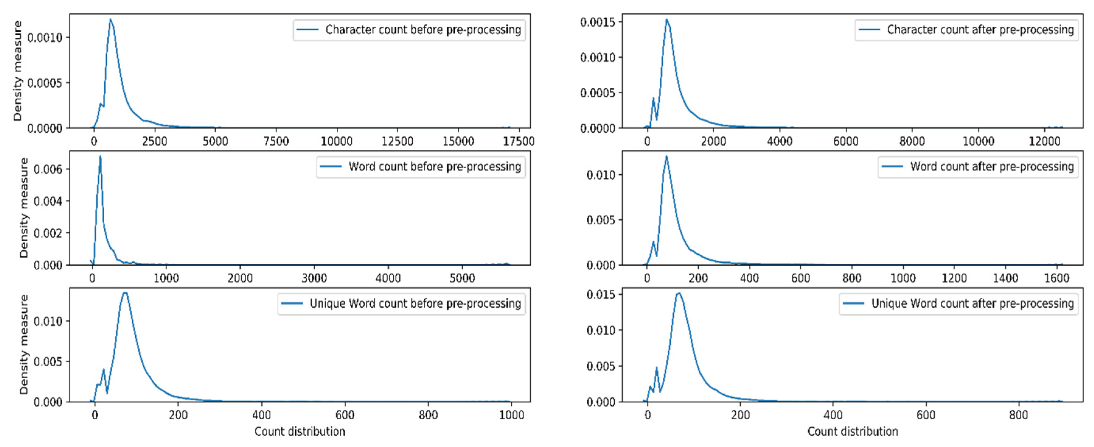
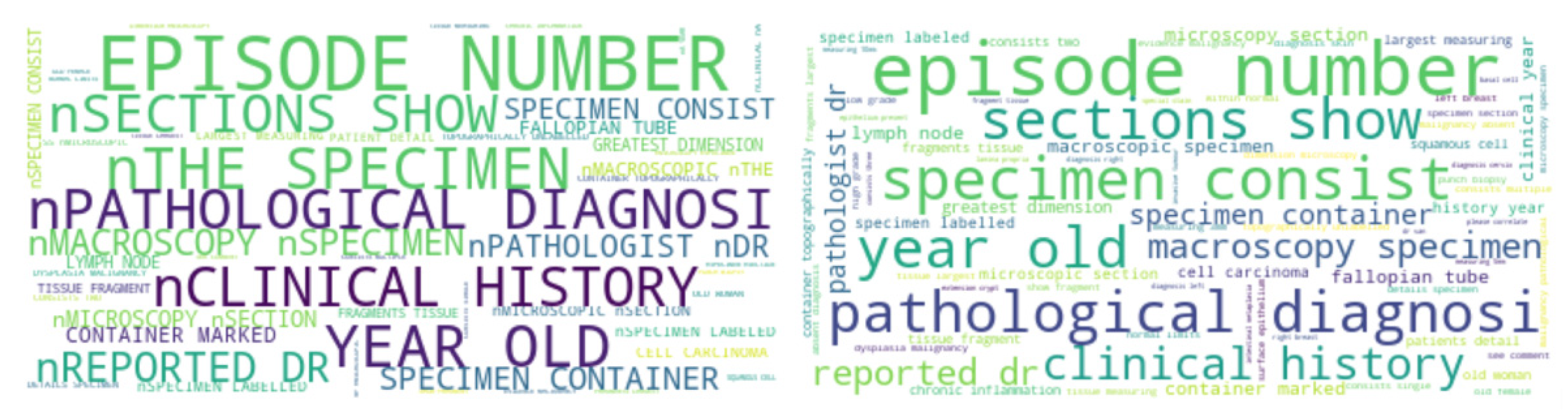
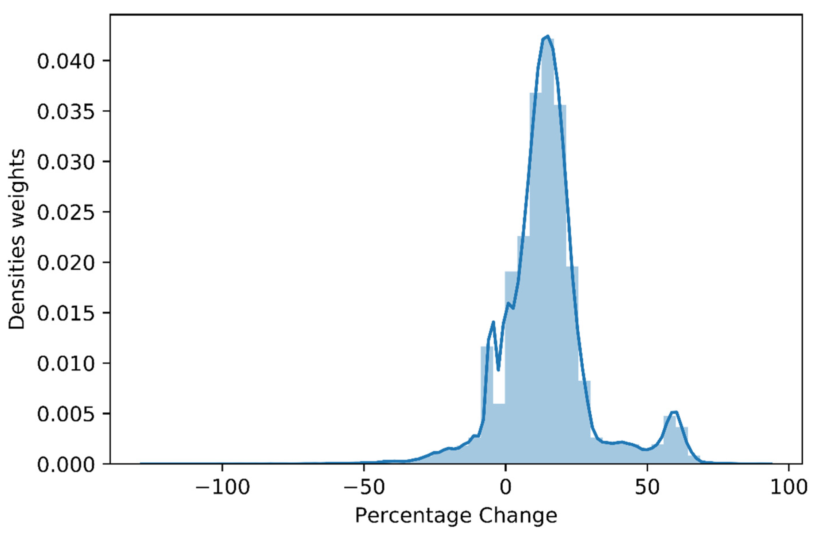
2.4. Pre-Processing
2.5. Feature Engineering
2.6. Classification
2.6.1. Gaussian Naïve Bayes (GNB)
2.6.2. Adaptive Boosting (AB)
2.6.3. Logistic Regression (LR)
2.6.4. Stochastic Gradient Descent (SGD)
2.6.5. K-Nearest Neighbor (KNN)
2.6.6. Support Vector Machine (SVM)
2.6.7. Decision Trees (DT)
2.6.8. Random Forest (RF)
2.7. Model Optimization
2.8. Evaluation
3. Results
3.1. Pre-Processing
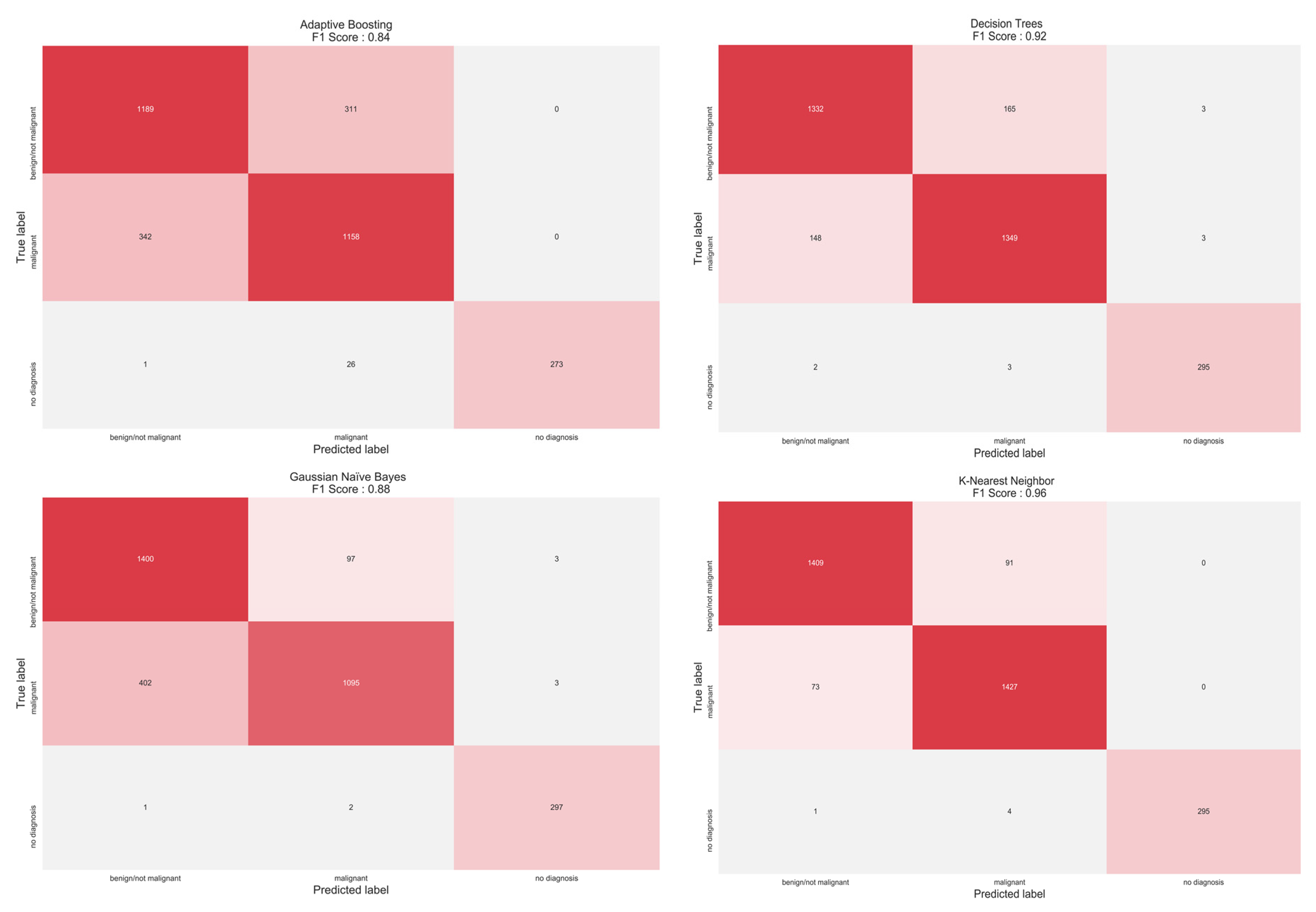
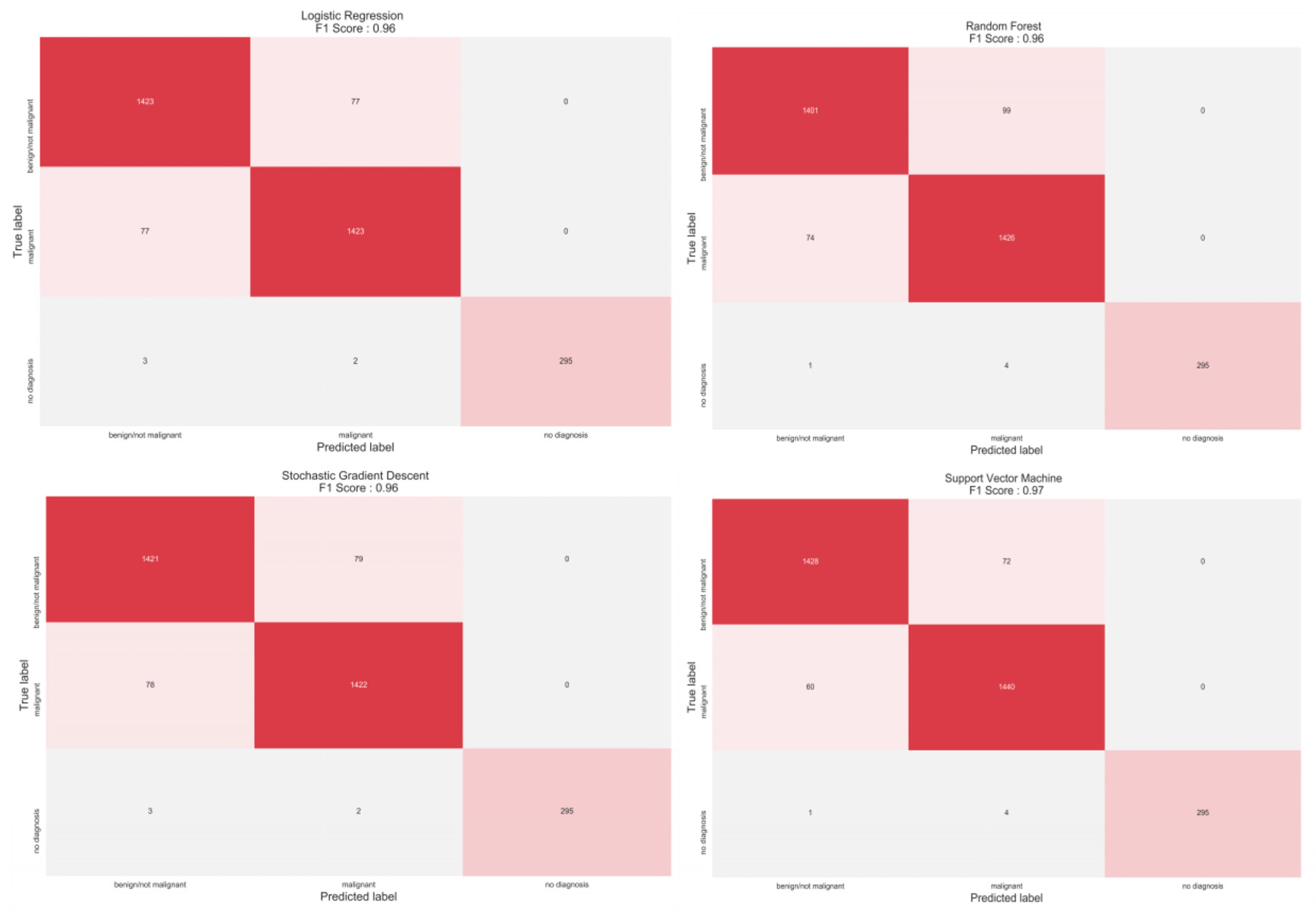
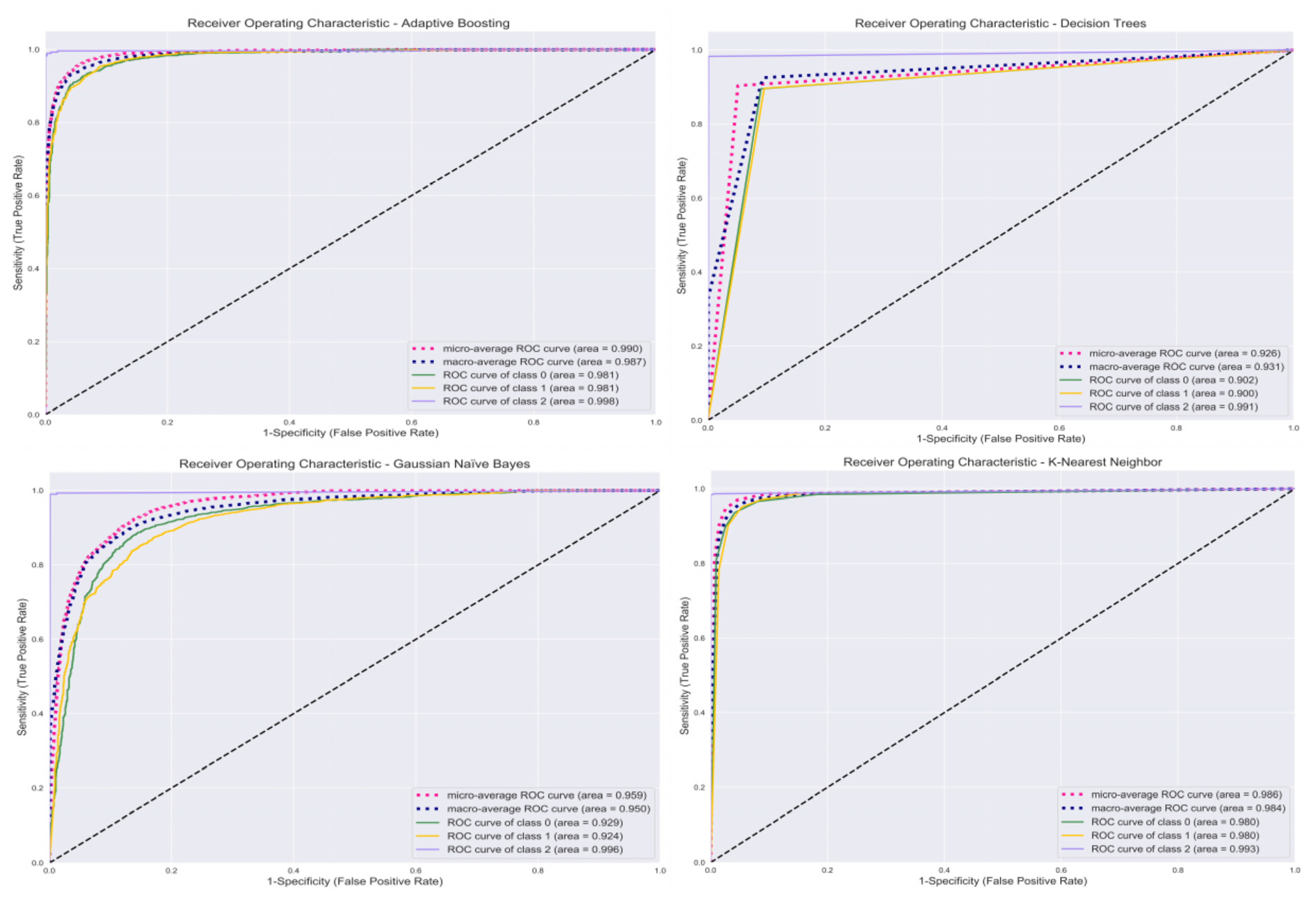
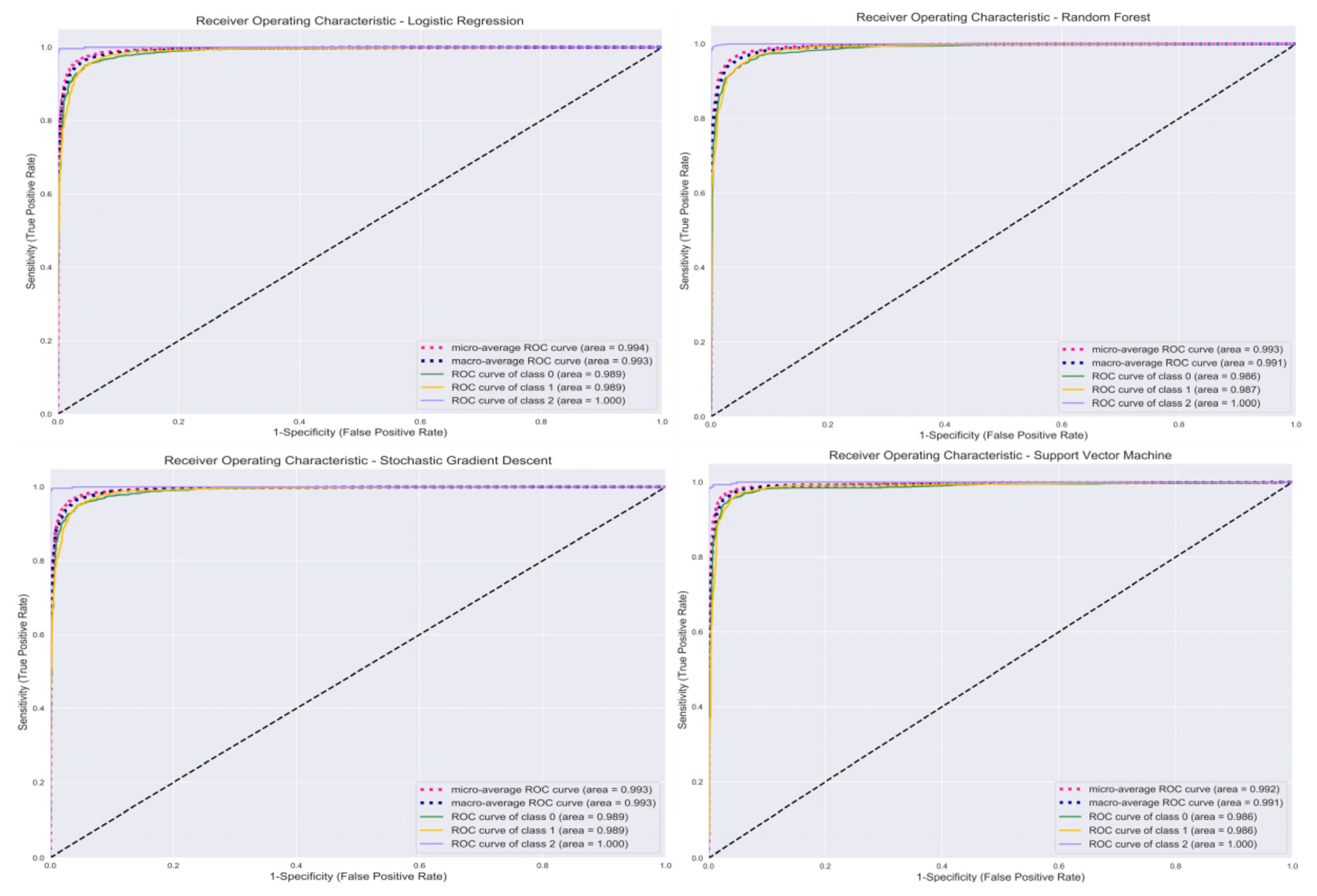
3.2. Classification
4. Discussion
5. Conclusions
Supplementary Materials
Author Contributions
Funding
Acknowledgments
Conflicts of Interest
Abbreviations
| SNOMED CT | Systematized Nomenclature of Medicine—Clinical Terms |
| ICD-O | International Classification of Diseases for Oncology |
| GridSearchCV | GridSearch Cross-Validation |
| SSA | Sub-Saharan Africa |
| SA | South Africa |
| NCR | South African National Cancer Registry |
| NHLS | National Health Laboratory Service |
| ML | Machine Learning |
| ID | Identification |
| SGD | Stochastic Gradient Descent |
| SVM | Support Vector Machine |
| AB | Adaptive Boosting |
| GNB | Gaussian Naïve Bayes |
| LR | Logistic Regression |
| DT | Decision Trees |
| KNN | K-Nearest Neighbor |
| RF | Random Forest |
| TF | Term Frequency |
| TF-IDF | Term Frequency Inverse Document Frequency |
| SVD | Singular Value Decomposition |
| LSA | Latent Sematic Analysis |
| BGD | Batch Gradient Descent |
| CM | Confusion Matrix |
| ROC | Receiver Operating Characteristics |
| AUC | Area Under Curve |
| TP | True Positive |
| TN | True Negative |
| FP | False Positive |
| FN | False Negative |
References
- Singh, E.; Underwood, J.M.; Nattey, C.; Babb, C.; Sengayi, M.; Kellett, P. South African National Cancer Registry: Effect of withheld data from private health systems on cancer incidence estimates. S. Afr. Med. J. 2015, 105, 107–109. [Google Scholar] [CrossRef] [PubMed] [Green Version]
- Singh, E.; Sengayi, M.; Urban, M.; Babb, C.; Kellett, P.; Ruff, P.; De Villiers, C.B. The South African National Cancer Registry: An update. Lancet Oncol. 2014, 15, e363. [Google Scholar] [CrossRef]
- Dube, N.; Girdler-Brown, B.; Tint, K.; Kellett, P. Repeatability of manual coding of cancer reports in the South African National Cancer Registry, 2010. S. Afr. J. Epidemiol. Infect. 2013, 28, 157–165. [Google Scholar] [CrossRef] [Green Version]
- Bray, F.; Parkin, D.M. Evaluation of data quality in the cancer registry: Principles and methods. Part I: Comparability, validity and timeliness. Eur. J. Cancer 2009, 45, 747–755. [Google Scholar] [CrossRef] [PubMed]
- Singh, E.; Ruff, P.; Babb, C.; Sengayi, M.; Beery, M.; Khoali, L.; Kellett, P.; Underwood, J.M. Establishment of a cancer surveillance programme: The South African experience. Lancet Oncol. 2015, 16, e414–e421. [Google Scholar] [CrossRef] [Green Version]
- Defossez, G.; Burgun, A.; Le Beux, P.; Levillain, P.; Ingrand, P.; Claveau, V.; Jouhet, V. Automated Classification of Free-text Pathology Reports for Registration of Incident Cases of Cancer. Methods Inf. Med. 2012, 51, 242–251. [Google Scholar] [CrossRef]
- O’Mara-Eves, A.; Thomas, J.; McNaught, J.; Miwa, M.; Ananiadou, S. Using text mining for study identification in systematic reviews: A systematic review of current approaches. Syst. Rev. 2015, 4, 5. [Google Scholar] [CrossRef] [PubMed] [Green Version]
- Harpaz, R.; Callahan, A.; Tamang, S.; Low, Y.; Odgers, D.; Finlayson, S.; Jung, K.; LePendu, P.; Shah, N.H. Text Mining for Adverse Drug Events: The Promise, Challenges, and State of the Art. Drug Saf. 2014, 37, 777–790. [Google Scholar] [CrossRef]
- Fleuren, W.W.; Alkema, W. Application of text mining in the biomedical domain. Methods 2015, 74, 97–106. [Google Scholar] [CrossRef]
- Rodriguez-Esteban, R.; Bundschus, M. Text mining patents for biomedical knowledge. Drug Discov. Today 2016, 21, 997–1002. [Google Scholar] [CrossRef] [PubMed]
- Zhu, F.; Patumcharoenpol, P.; Zhang, C.; Yang, Y.; Chan, J.; Meechai, A.; Vongsangnak, W.; Shen, B. Biomedical text mining and its applications in cancer research. J. Biomed. Inform. 2013, 46, 200–211. [Google Scholar] [CrossRef] [Green Version]
- Bui, D.D.A.; Zeng-Treitler, Q. Learning regular expressions for clinical text classification. J. Am. Med. Inform. Assoc. 2014, 21, 850–857. [Google Scholar] [CrossRef] [PubMed] [Green Version]
- Osborne, J.D.; Wyatt, M.; O Westfall, A.; Willig, J.; Bethard, S.; Gordon, G. Efficient identification of nationally mandated reportable cancer cases using natural language processing and machine learning. J. Am. Med. Inform. Assoc. 2016, 23, 1077–1084. [Google Scholar] [CrossRef] [PubMed]
- Bird, S.; Klein, E. Regular Expressions for Natural Language Processing; University of Pennsylvania: Philadelphia, PA, USA, 2006; pp. 1–7. Available online: http://courses.ischool.berkeley.edu/i256/f06/papers/regexps_tutorial.pdf (accessed on 2 May 2018).
- Hermawan, R. Natural Language Processing with Python; O’Reilly Media, Inc: Newton, MA, USA, 2011. [Google Scholar] [CrossRef]
- Spasic, I.; Livsey, J.; Keane, J.; Nenadic, G. Text mining of cancer-related information: Review of current status and future directions. Int. J. Med. Inform. 2014, 83, 605–623. [Google Scholar] [CrossRef] [PubMed]
- Kumar, S.; Goel, S. Enhancing Text Classification by Stochastic Optimization method and Support Vector Machine. Int. J. Comput. Sci. Inf. Technol. 2015, 6, 3742–3745. [Google Scholar]
- Bastanlar, Y.; Özuysal, M. Introduction to Machine Learning. Adv. Struct. Saf. Stud. 2013, 105–128. [Google Scholar] [CrossRef] [Green Version]
- Vural, S.; Wang, X.; Guda, C. Classification of breast cancer patients using somatic mutation profiles and machine learning approaches. BMC Syst. Biol. 2016, 10, 62. [Google Scholar] [CrossRef] [PubMed] [Green Version]
- Sarkar, D. Text Analytics with Python; Apress: New York, NY, USA, 2016. [Google Scholar]
- Navarre, S.W.; Steiman, H.R. Root-End Fracture During Retropreparation: A Comparison Between Zirconium Nitride-Coated and Stainless Steel Microsurgical Ultrasonic Instruments. J. Endod. 2002, 28, 330–332. [Google Scholar] [CrossRef] [PubMed]
- McCowan, I.; Moore, D.C.; Nguyen, A.N.; Bowman, R.V.; Clarke, B.E.; Duhig, E.E.; Fry, M.-J. Collection of Cancer Stage Data by Classifying Free-text Medical Reports. J. Am. Med. Inform. Assoc. 2007, 14, 736–745. [Google Scholar] [CrossRef]
- Kasthurirathne, S.N.; E Dixon, B.; Grannis, S. Evaluating Methods for Identifying Cancer in Free-Text Pathology Reports Using Various Machine Learning and Data Preprocessing Approaches. Stud. Health Technol. Inform. 2015, 216, 1070. [Google Scholar] [CrossRef]
- Nguyen, A.N.; Moore, J.; O’Dwyer, J.; Philpot, S. Automated Cancer Registry Notifications: Validation of a Medical Text Analytics System for Identifying Patients with Cancer from a State-Wide Pathology Repository. Available online: https://0-www-ncbi-nlm-nih-gov.brum.beds.ac.uk/pmc/articles/PMC5333242/pdf/2496545.pdf (accessed on 13 July 2019).
- van Guido, R.P. Development Team. The Python Language Reference; Python Software Foundation: Wilmington, DE, USA, 2013; p. 11. Available online: http://docs.python.org/2/reference/lexical_analysis.html (accessed on 28 October 2019).
- Anaconda, I. Anaconda Documentation, Release 2.0, Read Docs. Available online: https://docs.anaconda.com/anaconda/navigator/ (accessed on 27 October 2019).
- Ipython, T.; Team, D. IPython Documentation. Read Docs 2011, 3, 293–299. Available online: http://ipython.scipy.org/moin/ (accessed on 3 July 2019).
- Wes McKinney& PyData Development Team. Pandas: Powerful Python Data Analysis Toolkit Release 0.25.0. p. 2827. Available online: https://pandas.pydata.org/pandas-docs/stable/pandas.pdf (accessed on 19 July 2019).
- Gold, B.; Cankovic, M.; Furtado, L.V.; Meier, F.; Gocke, C.D. Do circulating tumor cells, exosomes, and circulating tumor nucleic acids have clinical utility? A report of the association for molecular pathology. J. Mol. Diagn. 2015, 17, 209–224. [Google Scholar] [CrossRef] [PubMed] [Green Version]
- Hosoya, H.; Pierce, B.C. Regular expression pattern matching for XML. J. Funct. Program. 2003, 13, 961–1004. [Google Scholar] [CrossRef] [Green Version]
- Pedregosa, F.; Varoquaux, G.; Gramfort, A.; Michel, V.; Thirion, B.; Grisel, O.; Blondel, M.; Prettenhofer, P.; Weiss, R.; Dubourg, V.; et al. Duchesnay, Fré. Scikit-Learn: Machine Learning in Python. J. Mach. Learn. Res. 2011, 12, 2825–2830. Available online: http://scikit-learn.sourceforge.net (accessed on 6 August 2020).
- National Health Laboratory Service. Annual Report; National Health Laboratory Service: Johannesburg, South Africa, 2017; Available online: http://www.nhls.ac.za/assets/files/an_report/NHLS_AR_2018.pdf (accessed on 18 July 2019).
- Miceli, P.A.; Blair, W.D.; Brown, M.M. Isolating Random and Bias Covariances in Tracks. In Proceedings of the 2018 21st International Conference on Information Fusion (FUSION), Cambridge, UK, 10–13 July 2018. [Google Scholar]
- Mujtaba, G.; Shuib, N.L.M.; Raj, R.G.; Rajandram, R.; Shaikh, K.; Al-Garadi, M.A. Automatic ICD-10 multi-class classification of cause of death from plaintext autopsy reports through expert-driven feature selection. PLoS ONE 2017, 12, e0170242. [Google Scholar] [CrossRef]
- Kowsari, K.; Meimandi, K.J.; Heidarysafa, M.; Mendu, S.; Barnes, L.; Brown, D.; Meimandi, J. Text Classification Algorithms: A Survey. Information 2019, 10, 150. [Google Scholar] [CrossRef] [Green Version]
- B.C. O’Leary, C.M.; Watson, L.; D’Antoine, H.; Stanley, F. Singular Value Decomposition (SVD); Carnegie Mellon University: Pittsburgh, PA, USA, 2012; pp. 1–36. [Google Scholar]
- National Cancer Institute. International Classification of Diseases for Oncology, 3rd ed.; World Health Organization: Geneva, Switzerland, 2020. [Google Scholar]
- Schapire, R.E. Using output codes to boost multiclass learning problems. In Proceedings of the Fourteenth International Conference on Machine Learning, San Francisco, CA, USA, 8–12 July 1997; pp. 313–321. [Google Scholar]
- Lin, C.-J.; Weng, R.C.; Keerthi, S.S.; Weng, R.C. Trust region Newton methods for large-scale logistic regression. In Proceedings of the 24th International Conference on Real-Time Networks and Systems—RTNS ’16; Association for Computing Machinery: New York, NY, USA, 2007; Volume 9, pp. 627–650. [Google Scholar] [CrossRef]
- Bottou, L. Large-Scale Machine Learning with Stochastic Gradient Descent. In Proceedings of COMPSTAT’2010; Physica-Verlag HD: Paris, France, 2010; pp. 177–186. [Google Scholar]
- Sharma, A. Guided Stochastic Gradient Descent Algorithm for inconsistent datasets. Appl. Soft Comput. 2018, 73, 1068–1080. [Google Scholar] [CrossRef]
- Lin, M.; Fan, B.; Lui, J.C.; Chiu, D.-M. Stochastic analysis of file-swarming systems. Perform. Eval. 2007, 64, 856–875. [Google Scholar] [CrossRef]
- Riggs, R.J.; Hu, S.J. Disassembly Liaison Graphs Inspired by Word Clouds. Procedia CIRP 2013, 7, 521–526. [Google Scholar] [CrossRef] [Green Version]
- Bray, F.; Jemal, A.; Grey, N.; Ferlay, J.; Forman, D. Global cancer transitions according to the Human Development Index (2008–2030): A population-based study. Lancet Oncol. 2012, 13, 790–801. [Google Scholar] [CrossRef]
- Koopman, B.; Karimi, S.; Nguyen, A.; McGuire, R.; Muscatello, D.; Kemp, M.; Truran, D.; Zhang, M.; Thackway, S. Automatic classification of diseases from free-text death certificates for real-time surveillance. BMC Med. Inform. Decis. Mak. 2015, 15, 53. [Google Scholar] [CrossRef] [PubMed] [Green Version]


| Model | Parameters |
|---|---|
| SGD | Alpha = 0.0001, average = False, class_weight = None, early_stopping = False, epsilon = 0.1, eta0 = 0.0, fit_intercept = True, l1_ratio = 0.15, learning_rate = ‘optimal’, loss = ‘log’, max_iter = 1000, n_iter_no_change = 5, n_jobs = None, penalty = ‘l2′, power_t = 0.5, random_state = None, shuffle = True, tol = 0.001, validation_fraction = 0.1, verbose = 0, warm_start = False |
| RF | bootstrap = True, ccp_alpha = 0.0, class_weight = None, criterion = ‘gini’, max_depth = None, max_features = ‘auto’, max_leaf_nodes = None, max_samples = None, min_impurity_decrease = 0.0, min_impurity_split = None, min_samples_leaf = 1, min_samples_split = 2, min_weight_fraction_leaf = 0.0, n_estimators = 100, n_jobs = None, oob_score = False, random_state = None, verbose = 0, warm_start = False |
| SVM | C = 1.0, break_ties = False, cache_size = 200, class_weight = None, coef0 = 0.0, decision_function_shape = ‘ovr’, degree = 3, gamma = ‘scale’, kernel = ‘rbf’, max_iter = −1, probability = True, random_state = None, shrinking = True, tol = 0.001, verbose = False |
| KNN | algorithm = ‘auto’, leaf_size = 30, metric = ‘minkowski’, metric_params = None, n_jobs = None, n_neighbors = 5, p = 2, weights = ‘uniform’ |
| AB | algorithm = ‘SAMME.R’, base_estimator = None, learning_rate = 1.0, n_estimators = 50, random_state = None |
| DT | ccp_alpha = 0.0, class_weight = None, criterion = ‘gini’, max_depth = None, max_features = None, max_leaf_nodes = None, min_impurity_decrease = 0.0, min_impurity_split = None, min_samples_leaf = 1, min_samples_split = 2, min_weight_fraction_leaf = 0.0, presort = ‘deprecated’, random_state = None, splitter = ‘best’ |
| LR | C = 1.0, class_weight = None, dual = False, fit_intercept = True, intercept_scaling = 1, l1_ratio = None, max_iter = 100, multi_class = ‘auto’, n_jobs = None, penalty = ‘l2′, random_state = 8, solver = ‘lbfgs’, tol = 0.0001, verbose = 0, warm_start = False |
| GNB | priors = None, var_smoothing = 1 × 10⁻⁹ |
| Report before Pre-Processing | Report after Pre-Processing | Text Class | Class |
|---|---|---|---|
| EPISODE NUMBER: \nXX1111111\n\n\nCLINICAL HISTORY: \nMULTIPLE GROWTH ABDOMEN RIGHT THIGH MOBILE 2 X 2CM. NIL SKIN CHANGE.\nSUBCUTANEOUS LESION RIGHT THIGH. LIPOMA.\n\n\nMACROSCOPY: \nSPECIMEN LABELED ¿LIPOMA RIGHT THIGH¿ CONSISTS OF A YELLOW FRAGMENT OF TISSUE MEASURING 15 X 8 X 5MM.\n\n\nMICROSCOPY:\nSECTION SHOWS LOBULES OF MATURE ADIPOCYTES WITH NUMEROUS INTERVENING SMALL BLOOD VESSELS. FIBRIN THROMBI ARE CONSPICUOUS WITHIN THE VESSELS. THERE IS NO EVIDENCE OF ATYPIA OR MALIGNANCY.\n\nPATHOLOGICAL DIAGNOSIS:\nSUBCUTANEOUS TISSUE OF RIGHT THIGH, EXCISIONAL BIOPSY: ANGIOLIPOMA.\n\nREPORTED BY: DR YYYYYY\n | episode number: xx1111111 clinical history: multiple growth abdomen right thigh mobile 2 × 2 cm nil skin change subcutaneous lesion right thigh lipoma macroscopy: specimen labeled lipoma right thigh consists yellow fragment tissue measuring 15 × 8 × 5 mm microscopy: section shows lobules mature adipocytes numerous intervening small blood vessels fibrin thrombi conspicuous within vessels no evidence atypia malignancy pathological diagnosis: subcutaneous tissue right thigh excisional biopsy: angiolipoma reported by: dr yyyyyy | Non-malignant | 0 |
| EPISODE NUMBER: \nXX2222222\n\n\nCLINICAL HISTORY: \nSKIN CANCER LEFT LOWER LEG. LONG STITCH = LATERAL, SHORT STITCH = SUPERIOR.\n\n\nMACROSCOPY:\nSPECIMEN LABELED ¿BCC LEFT LEG¿ CONSISTS OF AN ELLIPSE OF SKIN WITH A LARGE POLYPOID ULCERATED TUMOR MEASURING 65MM IN THE LONG AXIS AND 45MM IN THE SHORT AXIS. THE ULCER MEASURES 35 X 30MM.\n\n\nMICROSCOPY: \nSECTIONS SHOW A MODERATELY DIFFERENTIATED KERATINIZING SQUAMOUS CARCINOMA.\nMARGINS: \nLATERAL SKIN MARGIN 4MM\nMEDIAL 6MM\nPROXIMAL 12MM\nDISTAL 10MM\nDEEP RESECTION MARGIN 4-5MM\n\n\nPATHOLOGICAL DIAGNOSIS:\nSKIN OF LOWER LEG, EXCISION: SQUAMOUS CARCINOMA\n\nREPORTED BY: PROF XXXXXX\n | episode number: xx2222222 clinical history: skin cancer left lower leg long stitch lateral short stitch superior macroscopy: specimen labeled bcc left leg consists ellipse skin large polypoid ulcerated tumor measuring 65 mm long axis 45 mm short axis ulcer measures 35 × 30 mm microscopy: sections show moderately differentiated keratinizing squamous carcinoma margins: lateral skin margin 4 mm medial 6 mm proximal 12 mm distal 10 mm deep resection margin 4–5 mm pathological diagnosis: skin lower leg excision: squamous carcinoma reported: prof xxxxxx | Malignant | 1 |
| EPISODE NUMBER: \nXX3333333\n\n\nCLINICAL HISTORY: \nBMT\n\n\n\nPATHOLOGICAL DIAGNOSIS:\nIMMUNOHISTOCHEMISTRY PERFORMED AT THE DEPARTMENT OF ANATOMICAL PATHOLOGY, GROOTE SCHUUR HOSPITAL.\n\nRETURNED TO REFERRING CENTRE FOR REPORTING.\n | episode number: xx3333333 clinical history: bmt pathological diagnosis: immunohistochemistry performed department anatomical pathology groote schuur hospital returned referring centre reporting | No Diagnosis | 2 |
| Character Count before Pre-Processing | Character Count after Pre-Processing | Word Count before Pre-Processing | Word Count after Pre-Processing | Unique Words before Pre-Processing | Unique Words after Pre-Processing | Percentage Change | |
|---|---|---|---|---|---|---|---|
| Row count | 60,083 | 60,068 | 60,083 | 60,068 | 60,083 | 60,068 | |
| mean | 1032.12 | 863.09 | 143.32 | 110.12 | 88.10 | 81.69 | 14.41 |
| Standard deviation | 832.17 | 667.63 | 154.34 | 87.82 | 54.05 | 47.76 | 15.79 |
| min | 1 | 0 | 1 | 0 | 1 | 0 | −125 |
| 25% | 626 | 538 | 74 | 67 | 60 | 57 | 6.67 |
| 50% | 836 | 702 | 105 | 89 | 79 | 74 | 13.79 |
| 75% | 1180 | 982 | 164 | 125 | 104 | 96 | 20 |
| max | 16,961 | 12,419 | 5613 | 1607 | 983 | 884 | 90.14 |
| Model | Accuracy (%) | Precision (%) | Recall (%) | F1-Score (%) |
|---|---|---|---|---|
| SVM | 96 | 97 | 97 | 97 |
| LR | 95 | 96 | 96 | 96 |
| KNN | 95 | 96 | 96 | 96 |
| SGD | 95 | 96 | 96 | 96 |
| RF | 95 | 96 | 96 | 96 |
| DT | 90 | 93 | 92 | 92 |
| GNB | 85 | 89 | 88 | 88 |
| AB | 79 | 85 | 82 | 84 |
| Dummy | 41 | 32 | 32 | 32 |
| Model | Predicted | Label before | Total | |||
|---|---|---|---|---|---|---|
| Non-Malignant | Malignant | No Diagnosis | No Label | |||
| SDG | Non-malignant | 5193 | 689 | 12 | 36,019 | |
| Malignant | 208 | 10,000 | 3 | 5831 | 16,042 | |
| No diagnosis | 0 | 1 | 1283 | 830 | 2114 | |
| Total | 5401 | 10,690 | 1298 | 42,680 | ||
| SVM | Non-malignant | 5192 | 351 | 8 | 32,662 | 38,213 |
| Malignant | 209 | 10,338 | 7 | 9188 | 19,742 | |
| No diagnosis | 0 | 1 | 1283 | 830 | 2114 | |
| Total | 5401 | 10,690 | 1298 | 42,680 | ||
| RF | Non-malignant | 5379 | 282 | 1 | 29,199 | 34,861 |
| Malignant | 22 | 10,408 | 0 | 12,543 | 22,973 | |
| No diagnosis | 0 | 0 | 1297 | 938 | 2235 | |
| Total | 5401 | 10,690 | 1298 | 42,680 | ||
| KNN | Non-malignant | 5188 | 536 | 6 | 26,419 | 32,149 |
| Malignant | 213 | 10,153 | 8 | 15,425 | 25,799 | |
| No diagnosis | 0 | 1 | 1284 | 836 | 2121 | |
| Total | 5401 | 10,690 | 1298 | 42,680 | ||
| DT | Non-malignant | 5359 | 559 | 1 | 26,937 | 32,856 |
| Malignant | 40 | 10,126 | 1 | 13,900 | 24,067 | |
| No diagnosis | 2 | 5 | 1296 | 1843 | 3146 | |
| Total | 5401 | 10,690 | 1298 | 42,680 | ||
| AB | Non-malignant | 4142 | 2876 | 0 | 25,881 | 32,899 |
| Malignant | 1259 | 7810 | 17 | 15,834 | 24,920 | |
| No diagnosis | 0 | 4 | 1281 | 965 | 2250 | |
| Total | 5401 | 10,690 | 1298 | 42,680 | ||
| GNB | Non-malignant | 5000 | 3044 | 7 | 31,308 | 39,359 |
| Malignant | 398 | 7634 | 3 | 10,258 | 18,293 | |
| No diagnosis | 3 | 12 | 1288 | 1114 | 2417 | |
| Total | 5401 | 10,690 | 1298 | 42,680 | ||
| LR | Non-malignant | 5148 | 471 | 12 | 33,828 | 39,459 |
| Malignant | 253 | 10,218 | 3 | 8022 | 18,496 | |
| No diagnosis | 0 | 1 | 1283 | 830 | 2114 | |
| Total | 5401 | 10,690 | 1298 | 42,680 | ||
| Model | Misclassification Rates (%) | Approx. (Run Time) |
|---|---|---|
| SGD | 5.25 | 20 min |
| SVM | 3.31 | 2 h |
| RF | 1.75 | 8 h |
| KNN | 4.39 | 40 min |
| DT | 3.50 | 2 h |
| AB | 23.90 | 50 min |
| GNB | 19.94 | 4 min |
| LR | 4.26 | 10 min |
© 2020 by the authors. Licensee MDPI, Basel, Switzerland. This article is an open access article distributed under the terms and conditions of the Creative Commons Attribution (CC BY) license (http://creativecommons.org/licenses/by/4.0/).
Share and Cite
Olago, V.; Muchengeti, M.; Singh, E.; Chen, W.C. Identification of Malignancies from Free-Text Histopathology Reports Using a Multi-Model Supervised Machine Learning Approach. Information 2020, 11, 455. https://0-doi-org.brum.beds.ac.uk/10.3390/info11090455
Olago V, Muchengeti M, Singh E, Chen WC. Identification of Malignancies from Free-Text Histopathology Reports Using a Multi-Model Supervised Machine Learning Approach. Information. 2020; 11(9):455. https://0-doi-org.brum.beds.ac.uk/10.3390/info11090455
Chicago/Turabian StyleOlago, Victor, Mazvita Muchengeti, Elvira Singh, and Wenlong C. Chen. 2020. "Identification of Malignancies from Free-Text Histopathology Reports Using a Multi-Model Supervised Machine Learning Approach" Information 11, no. 9: 455. https://0-doi-org.brum.beds.ac.uk/10.3390/info11090455