A Frequent Pattern Conjunction Heuristic for Rule Generation in Data Streams


1
Research Department Marine Perception, German Research Center for Artificial Intelligence GmbH (DFKI), 26129 Oldenburg, Germany
2
Department of Computer Science, University of Reading, Reading RG6 6AY, UK
3
School of Computing and Digital Technology, Birmingham City University, Birmingham B4 7XG, UK
4
Faculty of Computer Science and Engineering, Galala University, Galala City 43511, Egypt
*
Author to whom correspondence should be addressed.
Information 2021, 12(1), 24; https://0-doi-org.brum.beds.ac.uk/10.3390/info12010024
Submission received: 3 December 2020
/
Revised: 30 December 2020
/
Accepted: 2 January 2021
/
Published: 9 January 2021
(This article belongs to the Special Issue Data Mining & Machine Learning Techniques for the Analysis of Stream Data)
Abstract
:This paper introduces a new and expressive algorithm for inducing descriptive rule-sets from streaming data in real-time in order to describe frequent patterns explicitly encoded in the stream. Data Stream Mining (DSM) is concerned with the automatic analysis of data streams in real-time. Rapid flows of data challenge the state-of-the art processing and communication infrastructure, hence the motivation for research and innovation into real-time algorithms that analyse data streams on-the-fly and can automatically adapt to concept drifts. To date, DSM techniques have largely focused on predictive data mining applications that aim to forecast the value of a particular target feature of unseen data instances, answering questions such as whether a credit card transaction is fraudulent or not. A real-time, expressive and descriptive Data Mining technique for streaming data has not been previously established as part of the DSM toolkit. This has motivated the work reported in this paper, which has resulted in developing and validating a Generalised Rule Induction (GRI) tool, thus producing expressive rules as explanations that can be easily understood by human analysts. The expressiveness of decision models in data streams serves the objectives of transparency, underpinning the vision of ‘explainable AI’ and yet is an area of research that has attracted less attention despite being of high practical importance. The algorithm introduced and described in this paper is termed Fast Generalised Rule Induction (FGRI). FGRI is able to induce descriptive rules incrementally for raw data from both categorical and numerical features. FGRI is able to adapt rule-sets to changes of the pattern encoded in the data stream (concept drift) on the fly as new data arrives and can thus be applied continuously in real-time. The paper also provides a theoretical, qualitative and empirical evaluation of FGRI.
1. Introduction
The advances in computing infrastructure and the emergence of applications that process a continuous flow of data records have led to the data stream phenomenon. Applications exist in science such as neuroscience, meteorology, and medicine as well as industry such as in aviation, finance, telecommunications and the chemical process industry. An important challenge in data mining is the learning process of large quantities of data through descriptive techniques. Contrary to predictive techniques, descriptive techniques aim to capture the relationships between features in order to explain the correlated relationships between any sub-sets of features to express interesting insights and patterns, rather than forecasting the value of a particular feature of unseen data instances.
A common approach to descriptive learning in data mining is frequent itemsets mining, which expresses many-many relationships between the items from a given number of itemsets. Association Rules learning is one of the techniques based on the concept of ‘Frequent Itemsets Mining’ to discover interesting relationships between items within itemsets. Association rules are in the general form of ‘IF THEN ’. For example, ‘IF a AND b THEN c’ where the presence of a and b are confirmed then the presence of c is highly likely with a minimum probability that is defined by the user in terms of support and confidence values of the rule. Further information about frequent itemsets mining as well as some important algorithms in this area are reviewed and discussed in the work of Christian Borgelt [1].
However, association rules only consist of binary values for each feature/item and this limits the flexibility and amount of information that a rule can represent [2,3]. An example of such an association rule in the context of market basket analysis could be IF {wine, cheese} THEN {bread, butter} indicating to an analyst if a customer buys wine and cheese the customer is also likely to by bread and butter. Here only the fact of presence or absence of an item/feature can be encoded but not an arbitrary value, which may be more informative of the feature/item.
Many real-life problems require more than the representation of a binary element to generate an output (where the output may also not be a binary value). For example, a temperature feature may be represented in the form of categorical values such as low, medium, high, or by a numerical value such as 20, 25.5, 30, etc. The antecedent of an association rule is a conjunction of a logical expression in the form of a feature-value’ pair and the specific form of this ‘feature-value’ pair depends on whether the feature is categorical or numerical. A rule representing such a more generalised and expressive relationship could be for example:
Assuming this rule is activated by a chemical process in a plant, it may express to the operator of the plant that the product flow is likely to be very low (between 1 and 5 litres per minute) and a pipe may be closed, because there is a high pressure and the temperature is between 60 and 15 degree Celsius. Based on this, the operator may investigate if the high pressure and temperature is caused by a blocked product release/overflow pipe. Please note that these are not predictive rules but rules that describe a frequent pattern in a data stream, i.e., the state of such a chemical plant/process.
The work on FGRI presented in this paper is motivated by the lack of algorithms available that can induce such expressive generalised rule-sets from data streams and also update the rule-set on the fly in real-time, when a concept drift is encountered. The Motivation for developing FGRI is the compelling need to unlock information of actionable value in a number of potential applications for which currently no data stream mining algorithms can be applied directly, some of which are outlined below. For example, techniques to predict network alarms and bottlenecks are employed in the UK national telecommunication network, however, the utilised methods often do not enable the tracing of the causality of such alarms [4]. A descriptive rule-set consisting of rules such as the above could enable applications to identify causality of alarms in telecommunication networks. However, such rule-sets would have to automatically adapt to concept drift due to unforeseen changes in the network structure, topology and external factors such as weather and demand. A further application could be to detect and quantify upcoming topics on Social Media such as on Twitter. Some work exists here using adaptive association rule mining techniques to induce and adapt rule-sets. Measuring the importance of upcoming rules and fading rules is used here to assess how recent/important a topic is and how it is developing. However, an adaptive rule-set with the ability to reflect numerical relationships such as those induced and maintained by FGRI, would enable more fine-grained tracing and detection of topics. In general the description of the states of systems is a possible type of application such as the aforementioned example with the states of a chemical plant. Here, large scale continuous chemical reaction facilities contain various sensors each representing a data feature. The sensor data is collected by a Process Control System [5]. A generalised rule-set would help the operator to identify important situations/states in the plant. However, such rule-sets would suffer from concept drift, i.e., due to changing outside temperatures, re-calibration of sensors, etc. The FGRI would be able to maintain an accurate and usable rule-set regardless of changes in the system.
This paper introduces and evaluates the first real-time method for concept drift adaptive generalised rule induction algorithm to represent frequent patterns, which is referred to as Fast Generalised Rule Induction (FGRI). The contributions of the paper are:
- 1
- An algorithm (FGRI) that can incrementally induce a set of generalised rules from a data stream in real-time, responsive to new data instances as these become available. The rules are explainable, expressive and can be applied on data streams with both, numerical and categorical features;
- 2
- A method in FGRI that is able to adapt the induced rule-set to concept drifts, i.e., changes of the pattern encoded in the data stream that occur in real-time. The method does not require a complete retraining of the rule-set but focuses on parts of the rule-set that are affected. It does this by removing rules that have become obsolete and adding rules for newly emerged concepts;
- 3
- A thorough evaluation of FGRI. This comprises: (i) an empirical evaluation on various data streams to examine the ability of FGRI to learn concepts in real-time and to adapt to concept drifts; (ii) a qualitative evaluation using real data to demonstrate the FGRI capability to produce explainable rule-sets; (iii) a theoretical complexity analysis to examine the FGRI scalability to larger and faster data streams.
Most rule learning algorithms for data streams to date aim at discovering comprehensible predictive models and this paper refers to these techniques as predictive rules learning, whereby a model consists of a set of rules induced from labelled training data and the model is used to predict the class label for unseen data examples. In contrast, the methodology proposed here, aims at finding expressive and thus understandable patterns described by individual rules; the methodology is referred to as descriptive rule learning and is designed for unlabelled data, as is the case for association rules. However, contrary to association rules the method can express a wider range of feature values (not just binary). In this context, if there is a special target feature, that the user always wishes to see in the output part of the rules, then this is referred to as classification. Whereas on the other hand the induced rules from FGRI are formulated in a more general context where the output part of the rule can be an arbitrary conjunction of ‘feature-value’ pairs. An important heuristic used in FGRI is that only most frequent feature-value pairs in categorical features are considered when inducing the rules. Such a heuristic not only speeds up the rule induction process, but also makes the descriptive rules an accurate representation of the current state of the system that rules are depicting.
The paper is organised as follows: Section 2 positions the proposed methodology in the context of related works and Section 3 describes the algorithm developed to induce modular generalised rules from training instances. Section 4 describes FGRI, the proposed algorithm to induce generalised adaptive rule-sets from streaming data directly and Section 5 provides an empirical and qualitative evaluation of FGRI. Finally, concluding remarks are set out in Section 6.
2. Related State-Of-The-Art
Charu Aggarwal [6] defines a data stream as a ‘sequence of data examples/instances’ which is produced at either a high rate, high volume or both. Some notable aspects can be used to distinguish conventionally stored data from data streams:
- –
- Data instances which arrive in real-time in any arbitrary sequence are to be processed in the order of their arrival; there is often no control over the order in which data instances arriving have to be seen, either within a data stream or across data streams.
- –
- Unbounded, the data instances are constantly arriving, and the exact quantity of the data instances is not known, also it is not known whether the stream would fit in the designated buffer or available hard drive space over time.
- –
- The concept in the data may change over time (concept drift).
Real-life applications involving streaming data can be seen in several domains including financial applications, computer networks, sensors monitoring and web applications. For example:
- –
- Popular on-line social networking sites such as Facebook, Twitter, and LinkedIn, offer their content tailored for each individual user. In order to do so, these services need to analyse huge amounts of data generated by the users in real-time to keep the content up to date [7].
- –
- Sensor Monitoring is a good example of applications in data stream mining [8]. More and more sensors are used in our personal daily lives and in industry. These sensors behave differently from traditional data sources because the data is periodically collected and discarded immediately, thus, the sensors do not keep a record of historical information. These unique challenges render traditional mining techniques and approaches inappropriate for mining real-time sensor data.
Given the above characteristics, conventional data mining approaches are not suitable for learning from data streams, because they were not designed to work directly on a rapid and continuous flow of individual data instances, as they are not inherently adaptive to changes temporally. There are notable algorithms in the literature that specifically deal with the unique challenges in building data mining models from streaming data in real-time. These models need to be adaptive to take concept drift into consideration, and thus need to be able to change when there are changes of the pattern encoded in the data stream. Various approaches exist to modify existing data mining algorithms for their application on data streams.
2.1. Windowing Techniques
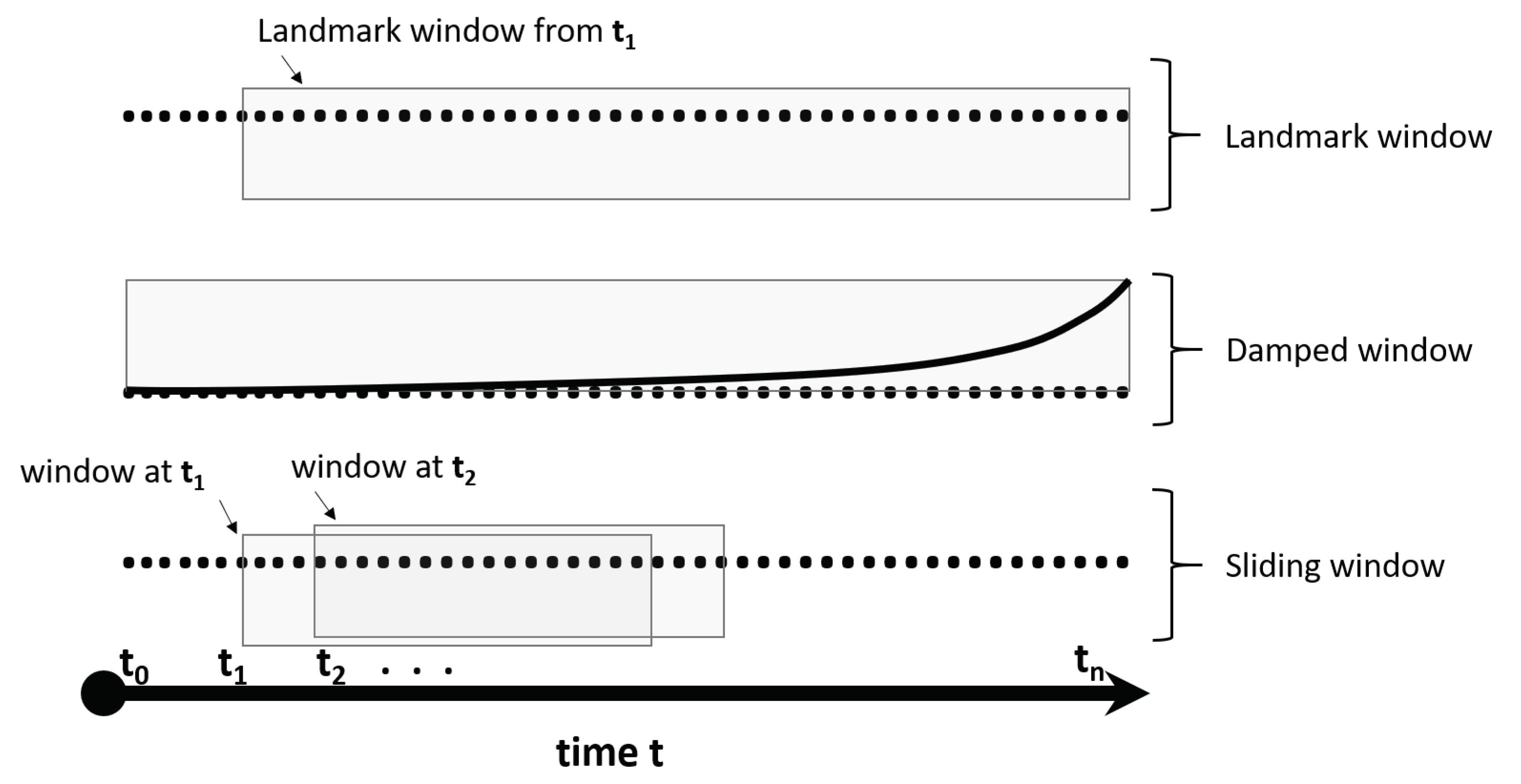
A well-known technique for adapting data mining algorithms to analysing data streams is windowing [9,10]. The idea of a windowing approach is to use an excerpt of typically the most recent and relevant data of the data instances from the stream for building and validating a data stream mining model. This excerpt is called a window. They can be broadly categorised in Landmark Windowing, Damped Windowing and Sliding Windows [11]. Figure 1 illustrates the three windowing categories.
The landmark window collects data instances at set epochal points, at which a new landmark is set, i.e., hourly, weekly, etc. When a new window is set, then the previous window including its data instances are deleted. Landmark windowing has been used in various real-time Data Stream Cluster Analysis algorithms such as CluStream, HPStream and StreamingKM++, etc. [12]. Siddique Ibrahim et al. [13] used this type of window to predict heart diseases.
The damped window associates a weight of recency to each data instance. Once the instance arrives the highest possible weight is assigned and thereafter decreased according to an ageing function. This model has been used in utility pattern mining, for example, Hyoju Nam et al. [14] proposed the DHUPL algorithm which mines high utility patterns using a list structure in which the difference in importance of data instances due to their arrival time is stored. Unil Yun et al. [15], developed an algorithm based on a high average utility pattern mining combined with damped windowing. Another example of the use of this technique is a network intrusion detection system [16] based on Data Stream Cluster Analysis and damped windowing.
The sliding can be of fixed or variable size w from a point in time t. As time passes the window slides and newly arriving data instances are included and older instances may be discarded. In its simplest form the sliding window is of fixed size and follows a first-in-first-out principle. A notable variable size sliding windowing technique is the ADaptive sliding WINdow method (ADWIN) [17]. ADWIN changes the window size based on observed changes. A Hoeffing bound based technique was proposed in [18] for mining classification rules, where the window size can adapt dynamically in order to provide sufficient data to capture the pattern being modelled and adapted. More recent techniques are, for example, the semi-supervised hybrid windowing ensembles [19] which are tailored for building ensemble classifiers from data streams. Unil Yun et al. [20] proposed an efficient and robust erasable pattern mining technique based on a sliding window approach in combination with a list structure. In [21], the authors developed a computationally efficient high utility pattern mining algorithm based on a sliding window approach.
Often windowing techniques are considered together with concept drift detection techniques in order to limit adaptation to cases where there is a change in the pattern encoded in the data.
2.2. Concept Drift Detection Techniques
Some common techniques here are the Drift Detection Method (DDM) [22] and the Early Drift Detection Method (EDDM) [23]. Both methods are based on error statistics and thresholding; whereas DDM performs well in detecting sudden concept drifts, it does not perform well in detecting gradual drifts for which, conversely, EDDM performs well. Some more recent developments are for example a framework which performs well on detecting a whole range of different types of drift for supervised algorithms [24], and a concept drift detection technique for unsupervised data mining based on Statistical Learning Theory (SLT) [25].
However, using windowing techniques in combination with concept drift detectors and batch data mining algorithms is a rather indirect and inflexible way to facilitate accurate model adaptation from data streams, as the models have to be retrained either periodically or when there is a concept drift. Therefore, data stream mining algorithms have been developed. These typically build adaptive models directly from streaming data without the need to retrain complete models. They can be broadly categorised into Predictive Adaptive DSM Algorithms and Descriptive Adaptive DSM Algorithms.
2.3. Predictive Adaptive DSM Algorithms
A notable family of predictive DSM algorithms are those based on the Hoeffding bound, known as Very Fast Machine Learning (VFML) techniques [26], with its first member being the Hoeffding tree, which is able to learn incrementally in real-time [27]. There have been various successors, such as the Concept Drift Very Fast Decision Tree (CVFDT), which is able to adapt the tree structure according to a concept drift and forget old concepts [28]. There are also highly expressive rule-based members of this family, i.e., Very Fast Decision Rules (VFDR) [29] or a more recent development termed Hoeffing Rules [18]. There are further recent expressive classifiers, i.e., Cano and Krawczyk [30] developed a rule-based algorithm using genetic programming that can adapt to concept drift, predictive fuzzy association rules [31] for real-time data; or rule-based granular systems for time series prediction [32].
Whereas the aforementioned methods generate expressive models, there are also less expressive techniques for predictive DSM. For example, ensemble-based approaches have been proposed to improve accuracy, enable fast recovery from concept drift and model switching. A representative here is the Evolutionary Adaptation to Concept Drifts (EACD) method [33], which uses evolutionary and genetic algorithms to adapt the ensemble to concept drift. Another DSM ensemble classifier is the Scale-free Network Classifier (SFNClassifier) [34], which represents the ensemble members as a single network. The Heterogeneous Dynamic Weighted Majority (HDWM) algorithm [35] proposes an ensemble approach that can intelligently switch between different types of base models. However, as non-expressive methods are less relevant for the work in this paper, they are not further discussed at this point.
2.4. Descriptive Adaptive DSM Algorithms
A large group of descriptive DSM algorithms are real-time cluster analysis methods. Although they are non-expressive by nature, they are mentioned here as they constitute an important type of descriptive Data Mining technique. An early representative here is CluStream [36] based on the notion of Micro-Clusters, which builds adaptive statistical summaries online while an offline component induces the actual spherical clusters for analytical purposes on demand. Various successors have been developed over the years, such as DenStream that can induce clusters of arbitrary shape on-demand [37]; or ClusTree [38] which supports agglomerative hierarchical cluster building. More recent developments here are evoStream [39] which uses evolutionary optimisation in idle times to refine clusters; SyncTree [40], which builds a hierarchical cluster structure and enables examining of cluster evolution; or the Evolving Micro-Clusters (EMC) method which is capable of determining new emerging concepts in the data stream [41]. However, there are very few expressive descriptive techniques capable to learning frequent patterns in real-time. Most are based on association rule mining and none of them are pure generalised rule induction techniques capable of handling tabular, numerical and categorical data features at the same time. For example, the Transaction-based Rule Change Mining (TRCM) technique [42], enables the detection of emerging, trending and disappearing rules, however, these rules are only applicable to tabular data. Tzung-Pei Hong et al. [43] developed an algorithm that generates association rules about concept drift patterns, but is limited to numerical data. Another rule-based algorithm, is again limited to tabular data but is able to adapt to concept drift [44].
2.5. Neural Networks for Data Stream Mining
The high accuracy of deep learning artificial neural networks has led to an increased research effort on applications using neural networks. In the area of Data Stream Mining, Spike Neural Networks (SNNs) are in use due to their ability to learn incrementally and continuously adapt responsive to new data. Furthermore, SNNs capable to learn time dependent relationships between features in the data stream. A recent example for SNNs in Data Stream Mining is [45]. The interested reader is referred to a survey about SNNs by Schliebs and Kasabov [46].
However, artificial neural networks are generally black-box models and the purpose of the research presented in this paper is to develop an explainable descriptive technique with rules containing expressive rule terms. As pointed out by the authors of [47], there has been an increase in research towards explainable ML, where some light is shed on black-box models, such as neural networks, through the extraction of a ‘post hoc’ model, for example such as in [48,49]. Rudin [47] points out further, that this is problematic, as explanations produced buy such ‘post hoc’ models are often not reliable and can even be misleading. They recommend using algorithms that are explainable and interpretable by nature, and thus are faithful to the model that they induce. Hence, artificial neural network techniques are not considered further for the work on FGRI presented in this paper.
2.6. Discussion
As can be seen in Section 2.3 and Section 2.4, earlier work on DSM aimed to address some of the aforementioned issues, i.e., there are expressive model generation techniques for predictive DSM. However, for descriptive expressive DSM to extract frequent patterns, such interpretable model and end-user friendly perspectives have been greatly neglected and are limited to very special cases such as transactional data. Features with different types of data cannot be handled at the same time. Hence, the users often do not trust DSM algorithms [50], which is a long-term unresolved issue.
Descriptive rules representing frequent patterns provide the users with more actionable information to make decisions, and thus enhance the trust in learning from streaming data sources. Rule-based data mining models are considered to be the most expressive models [18]. This paper introduces a novel technique to enable expressive exploration of streaming data in real-time in order to provide the end-user with an interpretable knowledge representation from streaming data in the form of descriptive rules.
Thus, the paper develops and evaluates a novel algorithm to induce a rule-set of descriptive generalised rules incrementally from raw data instances in real-time. The induced rules are not for special cases, but general and can be induced from raw data (comprising both categorical and numerical features) directly. Thereby the algorithm incrementally adapts the model (rule-set) over time to changes encoded in the data stream (concept drift), without the need to completely discard and re-induce the entire rule-set. To the best of the authors’ knowledge, this algorithm is the first of its kind to maintain and adapt generalised rules for streaming environments.
3. Generalised Rule Induction
This section describes the algorithm developed to induce modular generalised rules from training instances to express frequent patterns. The induced rules adhere to the following format:
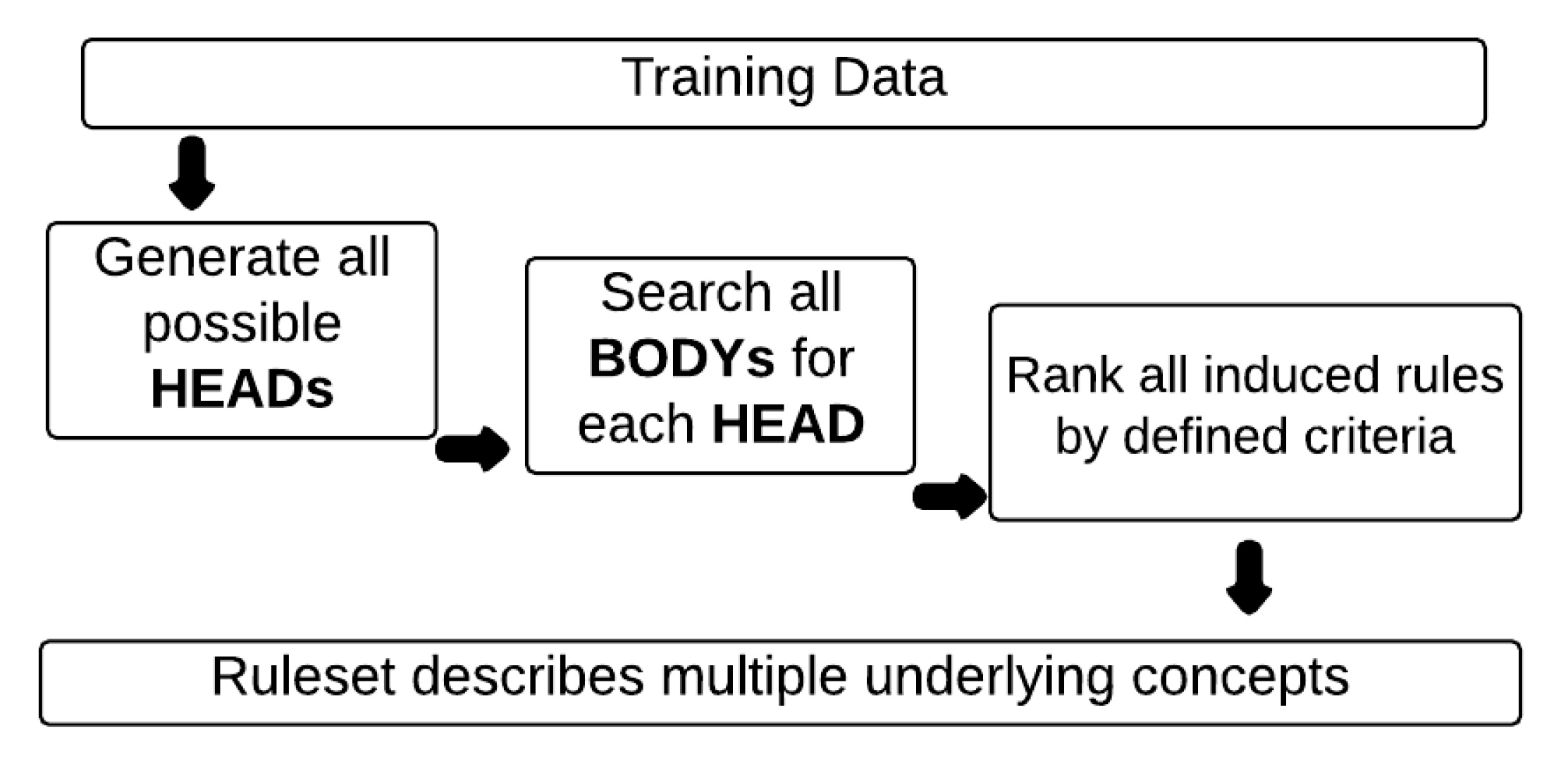
Figure 2 depicts the three processes of the proposed algorithm, which are (1) generating all possible HEADS, (2) for each HEAD generating all possible BODYs and (3) ranking of rules.
Both HEAD and BODY are represented as a conjunction of feature-value pairs where is a specific feature value, j is the feature index and i is the value index where there are n possible feature values. A feature can have either a finite (categorical) or an infinite (numerical) set of values. This paper refers to also as ‘rule term’. Rule terms of a finite (categorical) feature are expressed in the form of where . Rule terms of an infinite (numerical) feature are expressed in the form of , where . Section 3.2 describes how such rule terms are induced for numerical features. Loosely speaking, the algorithm aims to maximise the conditional probability of a particular HEAD and chooses rule terms accordingly.
3.1. Inducing Generalised Rules Using Separate and Conquer Strategy
A rule is made up of a maximum of n rule terms where n is the number of features in the data. In order to avoid contradicting rules, each feature can only appear once in the form of a rule term in a rule, no matter whether the feature was used in the HEAD or BODY of the rule. Furthermore, for a rule to be valid and meaningful it must have at least one rule term in the BODY and one in the HEAD part of the rule.
One possible way to find all possible conjunctions of rule terms is a brute-force exhaustive search [51], which can produce all possible conjunctions of terms up to a defined length l, this method does not use any heuristics for narrowing down the search space. This makes algorithms using this method very inefficient, and thus this approach is usually only discussed for academic purposes and theoretical studies. In this paper, covering or ‘Separate-and-Conquer’ search strategy is used to induce new rule terms for both BODY and HEAD. The concept of covering algorithms was first utilised in the 1960s by Michalski [52] for the AQ family of algorithms. However, the name ‘Separate-and-Conquer’ was not used until the 1990s by Pagallo and Haussler [53] when they attempted to formalise a theory to characterise this search strategy.
- –
- Separate part—Induce a rule that covers a part of the training data instances and remove the covered data instances from the training set.
- –
- Conquer part—Recursively learn another rule that covers some of the remaining data instances until no more data instances remain.
3.2. Inducing Rule Terms for Numerical Features Using Gaussian Distribution
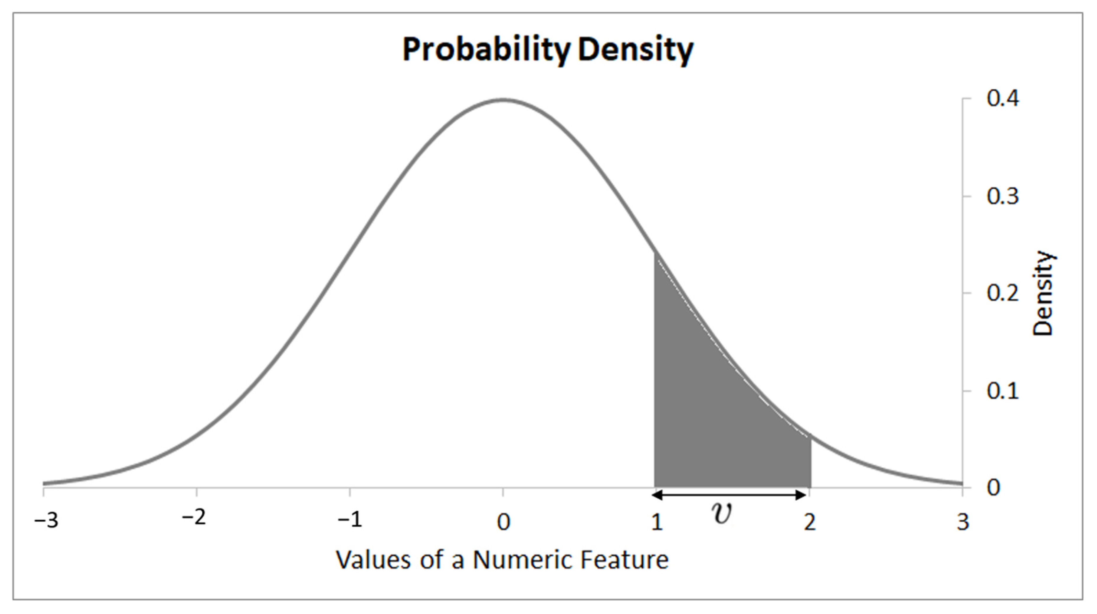
For a given HEAD the algorithm presented here provides a Gaussian distribution for each numerical feature as illustrated in Figure 3.
The generation of the rule HEADs is explained in Section 3.3. Assuming we have a set of HEADs , the most relevant value of a feature for a particular HEAD can be computed based on the Gaussian distribution of the feature values associated with this HEAD. The Gaussian distribution is calculated for a numerical feature with mean and variance from all feature values associated with HEAD, . The conditional density probability can be calculated by:
Next the posterior class probability , or equivalently is calculated to determine the probability of a HEAD for a valid value of continuous feature .
Then the probability of regions for these feature values, such that if then v belongs to a , is calculated. This does not necessarily capture the full details of the complex distribution of a numerical feature. However, it is computationally efficient in terms of processing time and memory consumption as the Gaussian distribution only needs to be calculated once. Subsequently the distribution only requires updates when instances are deleted from the training data due to the separate-and-conquer approach illustrated in Section 3.1. These updates are performed simply by re-calculating and of the distribution. According the central limit theorem [54,55], if a sample is large enough then it tends to be normally distributed regardless of the underlying distribution of the data. Thus, the algorithm assumes normally distributed numerical features as this work is concerned with the development of a rule induction algorithm for infinite streams of data. For more information and proofs about the Gaussian Probability Density function, the interested reader is referred to the work of Maria Isabel Ribeiro [56].
3.3. Inducing the HEAD of a Generalised Rule
In the current implementation, the HEAD only comprises rule terms induced from categorical features, where k is the number of all candidate rule terms and n is the number of features. In order to enable the user to inject domain knowledge, the maximum length of the HEAD can be set by the user. In addition, the implementation enables the user to specify which group of features is to be considered for the HEAD. By doing so, the user has the opportunity to use subjective measures of interestingness specific to their domain to influence the HEADs of the rules. In this case n would be the size of the group of features selected for generating HEADs. The number of possible rule term conjunctions for the HEAD is:
In order to avoid ambiguous rule terms each feature can only be used once in a rule.
Generating every possible permutation of rule terms can uncover most patterns encoded in the data, but it is also computationally very inefficient. Thus, for each feature, only one value is considered for the HEAD. In the current implementation, the candidate rule term of a feature with the highest frequency feature value is chosen. Alternatively, a feature value with the lowest frequency could be chosen; however, this is likely to result in many smaller rules (as lower frequency feature values cover less data instances). It is believed that many small rules are less convenient for the human analyst to interpret. The generation of all possible conjunctions of a HEAD (with the limitation described above) is described in Algorithm 1.
| Algorithm 1: Generate all possible HEAD conjunctions. |
D: original training data instances; : all possible terms (feature-value) from all features; : a collection of all possible conjunctions for HEAD; : number of maximum terms for conjunction; : a Head, represented by a conjunction of terms; : a collection of terms used for induced HEADs; Let ; Let
;  |
3.4. Inducing Rule BODYs for a HEAD
Algorithm 2 illustrates how all possible conditional parts (BODYs) for a particular HEAD are searched by using the separate-and-conquer strategy described in Section 3.1. The strategy maximises the conditional probability with which the BODY covers the HEAD of a rule. The algorithm aims to induce complete rules, which may potentially lead to a low coverage of data instances. Intuitively one may say that this can lead to overfitting of a rule/rule-set. In the case of predictive rules a low coverage may very well lead to overfitting. However, this may be different for descriptive rules, as illustrated in the example below:
- –
- Rule 1: IF AND THEN AND (covers 100%)
- –
- Rule 2: IF AND THEN AND (covers 98%)
- –
- Rule 3: IF AND THEN AND (covers 2%)
| Algorithm 2: Induce complete rules for each HEAD |
D: original training data instances; : The collection of all possible HEAD were generated in Algorithm 1; : A collection of all complete rules; : A list of all features in the dataset; : A list of used features;  |
From Rule 1 it is clear that if the reading from the sensor is as stated, then everything should be satisfactory. However, if then there is a high probability that the system was halted, and the temperature was high as it is in Rule 2. However, Rule 3 also contains the rule term yet everything is satisfactory, Rule 3 represents about 2 percent of the training data, in this fictitious example. In a predictive task such a rule would normally be discarded. However, Rule 2 may represent the normal behaviour of the system while Rule 3 represents an unusual outlier situation, i.e., such as the sensor itself is faulty. In a descriptive context, Rule 3 should be retained for further investigation by the analyst.
Overfitting is a fundamental problem for all learning algorithms [51]. In other words, overfitting means that learnt rules fit the training data very well which may result in inaccurate descriptions in unseen data instances. Typically, this problem occurs when the search space is too large. The reasons for overfitting are very diverse and can range from a constructed model that does not represent relevant domain characteristics to incomplete search spaces. One common problem is that real-world data usually contains noise such as erroneous or missing data instances.
A complete rule is not necessarily wrong, as it could also be an indicator of an unusual and thus interesting pattern in the data. Therefore, descriptive rule-sets retain all rules but rank them according to various metrics such as coverage, accuracy, interestingness, etc.
3.5. Pruning of Rules
In the proposed algorithm, a pre-pruning method was used to avoid overfitting during rule construction. It was decided to use rule length restriction as a pre-pruning method because of its simplicity and effectiveness as can be seen in our experimental evaluation in Section 5. However, if a more sophisticated pruning method for fine-tuning is desired, online or pre-pruning methods would be appropriate as the FGRI rule-set is not static, but constantly evolves over time. For example, an online pruning method that could be adapted to FGRI is the J-Pruning method [57]. J-Pruning measures the theoretical information content of a rule as it is being induced and stops inducing rule terms at the maximum theoretical information content of the rule. J-Pruning is not limited to a particular class label feature, and thus applicable to generalised rules. However, the development of a new rule pruning method is outside the scope of this research.
4. FGRI: Fast Generalised Rule Induction from Streaming Data
This section highlights the development of the proposed Fast Generalised Rules Induction algorithm conceptually. It is believed that this is the first kind of algorithm that is specifically designed to generate generalised rules from streaming data in real-time.
4.1. Real-Time Generalised Rules Induction from Streaming Data
The algorithm is based on a sliding window approach. A summary of windowing approaches including the sliding window approach is given in Section 2.1. A landmark window approach is not applicable to FGRI, as it is dependent on the application domain, and the objective of FGRI is to develop a generic algorithm that can be used in various contexts. A damped window approach is also not desirable, as it does not discard old data instances completely which will have negative computational implications on potentially infinite data streams. Sliding window approaches have been used successfully in various algorithms for streaming data including rule based predictive techniques, such as in [18,29].
Broadly speaking, when a sliding approach is used, the data instances in a window can be utilised for various tasks [58,59]:
- –
- To detect change/concept drift detection by using a statistic test to compare the underlying model between two different sub-windows.
- –
- To obtain updated statistics from recent data instances.
- –
- To rebuild or revise the learnt model after data has changed.
In addition, by using the sliding window approach, algorithms are not affected by stale data and an efficient amount of memory can be appropriately estimated [60]. However, the sliding window approach is not perfect and one of its main drawbacks is that the user will need to find a suitable window size before the learning process commences. This window size is then typically used throughout the entire learning process. The process of selecting a sliding window size is often made arbitrarily by the user or by trying different parameter settings and choosing the one that yields the best results from the evaluation metric used. A more robust and automatic method to choose a suitable sliding window size is desirable. This paper develops a sliding window approach embedded within FGRI which dynamically optimises the window size in real-time.
4.2. Inducing Generalised Rules from a Dynamically Sized Sliding Window
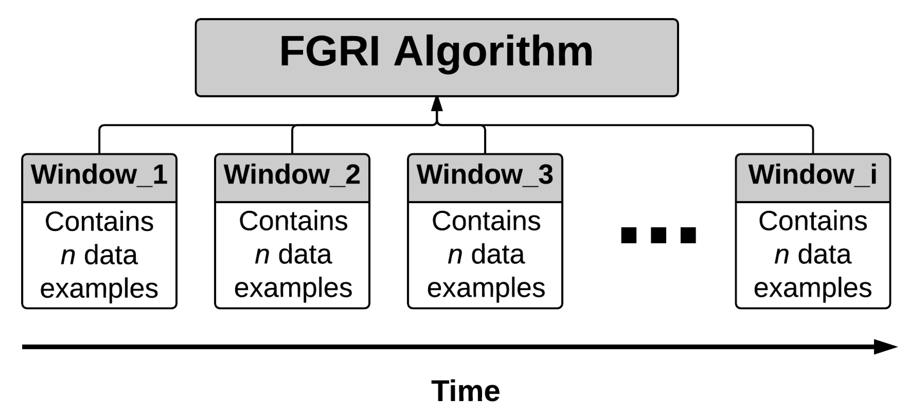
The complete algorithm to induce generalised decision rules from streaming data is proposed here with the combination of the algorithm as described in Section 3, a sliding window approach and a facility to adapt the window to an optimal size automatically and dynamically. For a better understanding of this Section, the sliding window approach is illustrated in Figure 4 and the FGRI pseudocode is available in Algorithm 3.
| Algorithm 3: Fast Generalised Rules Induction from streaming data |
 |
For this, the proposed algorithm makes use of the Hoeffding Inequality [27,29,61,62,63]. One can find the root of Hoeffding Inequality from the statistical literature of the 1960s. The properties of Hoeffding Inequality were utilised in streaming algorithms from the literature [26,29].
The proposed algorithm uses Hoeffding Inequality to estimate whether it is plausible to extend a particular decision rule or stopping the induction process for that rule. From the purely statistical perspective, ‘Hoeffding Inequality’ provides a statistical measurement of the confidence in the sample mean on n independent data instances where is the true mean and is the estimation of the true mean from an independent sample, then the difference in probability between and is bounded by:
where R is the possible range of the difference between and . From the bounds of the Hoeffding Inequality, it is assumed that with the confidence of , the estimation of the mean falls/lies within of the true mean. In other words:
From Equations (4) and (5) and solving for , a bound on how close the estimated mean is to the true mean after n observations, with a confidence of at least , is defined as follows:
For clarification, here is an example in a very simple scenario to show the property of the above Equation (6). A proof of the Hoeffding Bound or Hoeffding Inequality can be found [61] and its interpretation for use in data stream mining [27] and decision rule induction [18].
Problem: There is a vector of letters ‘A’ and ‘B’ and the probability of ‘A’ is exactly 0.30. In other words, if the vector size is 10,000 then there are 3000 times of ‘A’ and 7000 times of ‘B’.
Hypothesis: The concept of Equation (6) can be applied in this scenario to calculate the probability of ‘A’ from the given vector. Although, the real probability of ‘A’ is 0.3, let us assume that this value is not known, and it is necessary to calculate/estimate this value from a sample of values from the vector.
Defining Parameters: In this example, R = 1.0 because the probability of ‘A’ can only be between 0.0 and 1.0, therefore, the range, R, should be 1.0. and n are 0.05 and 200 respectively. However, n and are configurable and different values can be used.
Description: Based on the selected parameters, where n = 200, R = 1.0 and = 0.05 can then be calculated. Contextually, one can interpret that the estimated probability of ‘A’ from any 200 values sample from the initial vector of 10,000 should be smaller than with the certainty of 0.95. In other words, estimate the probability of ‘A’ from a sample of 200 random values from the original vector and repeat this process 100 times, then, at least 95 times the difference between the estimated probability of ‘A’ from the sample and the actual probability should be constrained by .
A bound based on ‘Hoeffding Inequality’ is used as a statistical metric to confirm whether a selected rule term from a given subset of data examples is also likely to be true if the rule term comes from an infinite set of data examples. In other words, for a given error, an extracted rule term from a much smaller and thus more manageable subset would be identical to that extracted from a much larger set of data examples.
An example of the use ‘Hoeffding Inequality’ can be described as in the following process:
1. Irrespective of whether we start inducing a rule term for either BODY or HEAD part we always start with all the training data instances from the window.
2. A heuristic is calculated for all possible rule terms at each iteration. Depending on whether a rule is induced for the BODY or the HEAD part then the coverage or conditional probability would be the corresponding heuristic.
3. As shown in Figure 5, the subset of data instances is reduced after each iteration, or after a new rule term is added to the rule being induced.
4. In a traditional ‘separate-and-conquer’ approach as in inducing a rule from static data, the process in Step 3 is repeated until the rule being induced covers 100% of data instances of the subset. However, this is where the Hoeffding Bound is effectively used in the algorithm. The algorithm will stop inducing/adding new rule terms as soon as the condition of ‘Hoeffding bound’ is not satisfied.
5. For the iteration as shown in Figure 5, a heuristic value, , is calculated for all possible rule terms. Let and be the best and second-best feature-value pair respectively of all calculated heuristic values then is as follows:
6. After any given iteration, if as in Equation (6) then the induction process of the rule is stopped.
4.3. Removing Obsolete Rules
Unless specified differently, all learnt rules are kept throughout the learning phase, but one can limit the number of rules at any given time by filtering out the rules with the lowest statistical metrics. For descriptive applications, multiple modular rules are useful when deeper examination of the emergent rule-set is deemed warranted. However, for a predictive application, then rules with a high misclassification rate ought to be removed. For each rule produced, there are statistical metrics that are maintained and updated after a new instance is seen:
For each rule produced, the following constitute the set of statistical metrics that are maintained and updated after each new rule instance is learnt.
- –
- True Positive Rate;
- –
- False Positive Rate;
- –
- Precision;
- –
- Recall;
- –
- F1-Score.
F1-Score is used as a default metric to rank descriptive rules, so that the top ‘k’ most meaningful rules can easily be extracted from the induced rule-set.
5. Evaluation
Experimental evaluations are presented in this section, and case studies for the algorithms realised in Section 3 and Section 4. The evaluation method employed uses a common evaluating technique for streaming data called Prequential Testing [29,64,65]. The algorithms were implemented in Java as an extension for WEKA and MOA [58]. The details and downloadable source code can be found on the project website (https://moa.cms.waikato.ac.nz/).
To date no other algorithms have been developed that are directly comparable to the algorithm presented by this study for the representation of generalised rules and to support adaptation to concept drifts in real-time. However, a thorough analysis and experiments are performed aiming to showcase the scalability, efficiency and effectiveness of the proposed algorithm both quantitatively and qualitatively.
5.1. Datasets
Both, artificial (stream generators in MOA) and real datasets are used in the experiments:
The Random Tree Generator [27] is based on a randomly generated decision tree and the number of features and classes can be specified by the user. New instances are generated by assigning uniformly distributed random values to features and the class label is determined using the tree. Because of the underlying tree-structure, decision-tree-based classifiers should perform better on this stream. Two versions of this data stream have been generated, one with five categorical and five continuous features, and three classifications called RT Generator 5-5-3, and the other also with 3 classifications but no categorical and only four continuous features called RT Generator 0-4-3. Both versions comprised 500,000 instances. The remaining settings were left at their default values, which are a tree random seed of 1, instance random seed option of 1, five possible values for each categorical feature, a maximum tree depth of 5; minimum tree level for leaf nodes of 3, and the fraction of leaves per level from the first leaf Level onward is 0.15.
The SEA Generator [65] generates an artificial data stream with two classes and three continuous features, whereas one feature is irrelevant for distinguishing between the two classes. This data generator has been used in empirical studies [29,66,67]. The default generator settings were used for this evaluation, which are concept function 1, a random instance seed of 1, enabling unbalanced classes and a noise level of 10%. 500,000 instances were generated.
The STAGGER Generator [68], describes a simple block world with three features that represent shapes, colour and size and concept drift is achieved through substitutions. It is commonly used as benchmark dataset [27,69,70,71].
Airlines, actually the Airlines Flight dataset, was created based on the regression dataset by Elena Ikonomovska, which was extracted from Data Expo 2009, consisting of about 500,000 flight records, the task being to use the information of scheduled departures to predict whether a given flight will be delayed. The dataset comprises three continuous and four categorical features. The dataset was also used in one of Elena Ikonomovska’s studies on data streams [72]. This real dataset was downloaded from the MOA website (http://moa.cms.waikato.ac.nz/datasets/) and used without any modifications.
Nursery [73], more expressively, the Nursery Admissions dataset, is extracted from a hierarchical decision model, which was designed to rank applications for nursery schools in Ljubljana, Slovenia over several years in 1980s. A set of 12,960 data instances was used from the Nursery Admissions dataset to extract rules. This has been used previously for empirical evaluation of Data Stream Mining algorithms [74].
5.2. Complexity Analysis of FGRI
In order to assess the applicability of FGRI on fast data streams, a time complexity analysis is provided.
It should be noted that the FGRI algorithm is a new type of analysis technique for data streams, and thus has no comparator techniques to date. FGRI produces descriptive rules from raw data instances incrementally and automatically updates the resulting descriptive rule-set in real-time, in responsive to emerging concept drifts in real data. As there are no algorithms of this kind for the real-time analysis of Data Streams yet, this complexity analysis is seen as a baseline against which future algorithms of this kind can be compared.
There are three components of FGRI that process data instances from the stream, and thus need to be analysed: (1) The validation of rules, (2) generation of rule HEADs, and (3) the induction of the rule body for each rule HEAD. In this analysis, the number of data instances is denoted N and the number of features M, which is constant.
With respect to component (1), this is in its worst case, a linear operation with respect to N, as each data instance and feature is at most used once to test a rule-set and only on the current rule-set active during the window the data instance was received. Hence the complexity of this component can described as . However, the user may limit the HEAD features manually or according to some subjective measure of interestingness, in which case the complexity with respect to the constant M would slow down the linear growth of the time complexity in N.
With respect to component (2), for categorical features ‘HEAD’ rule terms can be derived directly from the possible categorical values, whereas for numerical rule terms various calculations have to be performed, these are the calculation of , and (see Algorithm 2). Each received numerical instance would have to be used to update these statistics. Categorical features offer a limited finite number of possible ‘HEAD’ rule terms, which are simply the possible feature values. These are quite limited and do not have to be updated. Thus, the worst case is with respect to numerical features and is linear , as each data instance will be used to update the statistics for each feature.
With respect to component (3), the complexity of FGRI is based on updating , and for each feature. In an ideal case, there would be one feature that perfectly separates all the different rule HEADs, or simply all data instances would belong to the same rule HEAD. An average case is difficult to estimate, as the number of iterations of FGRI is dependent on the number of rules and rule terms induced, which in turn are dependent on the concept encoded in the data. However, it is possible to estimate the worst case. Furthermore, each feature will occur at most once (term) per rule, thus if it is contained in the HEAD already it will not be used for the Body part of the rule. In the worst case there will be one feature per HEAD and thus features will be used in total. Furthermore, in the worst case instances are encoded in a separate rule. The −1 is because if there is only one instance left, it cannot be used to divide the data further, which is needed for the rule induction process. The complexity (number calculations per instance) of inducing the rth rule is . The factor is the number of training instances not covered by the rules induced so far, as mentioned above, in the worst case, each rule covers only one training instance. These uncovered instances are used for the induction of the next rule. For example, the number of calculations for a term of the first rule , where the training data is still of size N, would be . The total number of calculations for the whole rule in this case would be as there are M rule terms and three properties to calculate (, and ). This, summed up for the whole number of rules, leads to:
this is equivalent to a complexity of . Please note that this estimate for the worst case is very pessimistic and unlikely to happen. In reality larger datasets often contain many fewer rules than there are data instances and in the case of FGRI, rules are limited to the k best rules. Hence, quadratic complexity is indeed highly unlikely for the average case.
5.3. The Expressiveness of Generalised Induced Rules
For a predictive learning task such as classification, the accuracy of the learnt model is normally referred to as correctly predicting the outcome for unseen data instances and a specific feature is only used in the ‘HEAD’ part. For example, in a classification task, more than one rule can cover a data instance and all the matched rules may not predict the same outcome, but the model still needs to settle on one outcome for the data instance and this is used as part of the evaluation process. Typically, a model will label an unseen data instance as one of the following scenarios:
- –
- True Positive ()—Both HEAD and BODY cover the data instance.
- –
- Abstained (A)—Neither HEAD nor BODY of a rule cover the data instance.
- –
- False Positive ()—BODY covers the data instance but the HEAD does not cover the data instance.
- –
- False Negative ()—BODY does not cover the data instance but the HEAD covers the data instance correctly.
Most evaluation metrics such as accuracy, sensitivity, specificity, precision, true positive rate, false positive rate, etc. are calculated based on true positive, true negative, false positive and false negative count. After a new data instance is evaluated the respective counts of true positive, true negative, false positive or false negative will be incremented by one and ‘total number of evaluated data instances’.
However, the performance of the algorithm is highly uncertain if these measurements are calculated for descriptive model evaluation as described above. The issues of concern here arise from: (i) whether or not an induced rule can correctly represent an unseen data instance and (ii) whether each rule contributes to the true positive, abstentions, false positive or false negative statistics rather than updating these measurements for each unseen data instance. Therefore, in the context of descriptive rule learning it is believed that, rather than considering the performance statistics derived from those on (i) and (ii) above, it is more appropriate to consider the absolute numbers of covered data instances by the induced rules [51,75].
Each rule should be interpreted and evaluated individually and the number of rules in the library is limited by default to 200. The number of relationships a person can meaningfully handle has been put between 150 to 250 [76]. Thus, a number of rules within this range, in this case 200, have been chosen. However, the rule limit can be set by the analyst to a different number. For all the experiments in this paper the default rule limit of 200 was used. Overly large rule-sets would also be time-consuming for the analyst to interpret. The rule limit does not interfere with the induction process nor the order of the rules. Therefore, the first 200 rules will always be the same even if a larger rule-set size were to be chosen. The algorithm learns and validates rules in real-time. In other words, invalid and out-of-date rules are removed and new rules which reflect current underlying concepts are added.
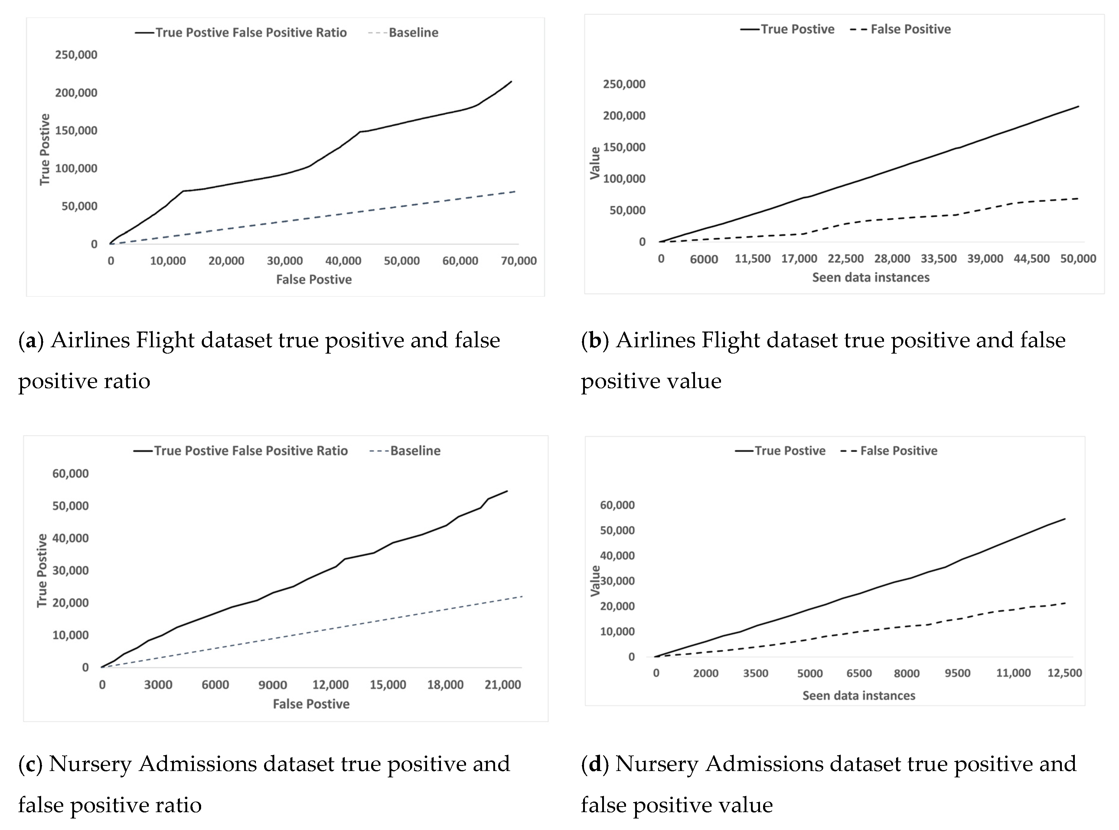
Figure 6 examines the evaluation metrics and on two real datasets Airlines Flight dataset and Nursery Admissions dataset. Here Figure 6a,c plot versus and the stream progresses steadily and proportionately from left to right along the horizontal axis and from bottom to top along the vertical axis respectively. For orientation a baseline has been included in the form of a dashed line. This is to indicate where a ratio of 1 would lie in the diagram. It is evident that the relationships are leaning more towards than indicating that the rules generated have learned the concept encoded in the data and are not random. Figure 6b,d plot the same and , but this time separately along the horizontal axis as the stream progresses. It can be seen that over time increases at a much higher rate than does, which shows that FGRI continues to adapt and improve the rule-set. This demonstrates that the learnt rules are statistically sound but whether the learnt rules are actually interesting in terms of domain information is subjective depending on many factors such as level of domain knowledge of theinterpreter, prior knowledge on the topic, etc.
The induced rule-sets are further examined from the perspective of their degree of interestingness. Both synthetic and real-life datasets are used in our experimental evaluations. How a data instance is generated by RandomTree and SEA synthetic data stream generators is understood as described. However, for a real-life dataset such as Airlines Flight dataset, the underlying patterns are unknown. A user can inspect induced rules directly from the Rules Library produced by the algorithm and can be confident that the rules correctly reflect the underlying pattern encoded in the data stream at any given time.
Some of the top rules in the 10,000 data instance snapshot are manually interpreted from the Airlines Flight dataset [72] to see if the rules can reveal any useful information. In a real-time streaming environment, there is often no control over the order of the flow of data instances and their speed. Therefore, if induced rules are interpreted at a 10,000 data instances snapshot then we can only expect the induced rules to describe patterns or concepts up to 10,000th data instance correctly. Data beyond this point should not be taken into account as future data has not been seen by the rule induction algorithm yet.
Airlines Flight dataset:
- –
- Rule 1: IF Delay THEN DayOfWeek .
- –
- Rule 2: IF Airline THEN Delay .
- –
- Rule 3: IF Airline THEN DayOfWeek .
- –
- Rule 4: IF Length THEN DayOfWeek .
- –
- Rule 5: IF AirportTo THEN Airline .
As shown above, the extracted rules are mostly self-explanatory. These rules were directly induced from the data and each rule was stored independently. However, these rules were confirmed with the first 10,000 data instances from the Airlines Flight dataset to see how the rules reflected the training data.
Airlines Flight dataset:
- –
- Rule 1: After first 10,000 data instance, out of 10,000 flights records are not delayed which is correctly suggested by this rule.
- –
- Rule 2: After first 10,000 data instances, 1139 records out of 1816, or 62, seen records for ‘WN’ airline are delayed.
- –
- Rule 3: The Airlines Flight dataset is sorted by ‘DayOfWeek’, so data for each day of the week is appended to each other. The first 10,000 records contain just records for all flights with ‘DayOfWeek = 3’.
- –
- Rule 4: Most of the flights have duration between 118 to 141 min. The first 10,000 records.
- –
- Rule 5: The majority of flights with destination as LAS are operated by WN airline. The first 10,000 records confirmed this.
The information from the inferred rules can be seen to be in line with the type of information extracted from the Data Expo competition (2009) where participants worked on a larger and more comprehensive Airlines Flight dataset. Unlike a classification task which only focuses on a specific feature, as shown above, the proposed algorithm can potentially reveal various forms of correlated information between features from training data in real-time as well as validating the rules to reflect the truth of the underlying concepts over time or at all/any times.
Another experiment was carried out, this time on the Nursery Admissions dataset [73], to show the effectiveness and robustness of the resulting rules in revealing expressive and actionable information from raw data. The data were extracted from a hierarchical decision model, which was designed to rank the applications for children to join the nursery schools in Ljubljana, Slovenia over several years in the 1980s. The data was used to understand the reasons behind the rejection decisions, which would have to be based on objective facts, as the rejected applications required objective decision making. The data contained the key features, which were used to make a final decision on each application. This consisted of three subcategories: (i) the occupation of the parents and the match to the nursery admission priorities, (ii) family structure and financial standing, and, (iii) social and health profile/status picture of the family [77].
Nursery Admissions dataset:
- –
- Rule 1: IF class = not_recom THEN health = not_recom.
- –
- Rule 2: IF parents = professional THEN has_nurs = very_crit.
- –
- Rule 3: IF health = priority THEN class = spec_prior.
- –
- Rule 4: IF form = complete THEN has_nurs = very_crit.
- –
- Rule 5: IF finance = convenient THEN parents = great_profession.
The above rules were discovered by the algorithm based on the 12,960 data examples from the Nursery Admissions dataset. The extracted rules were just as descriptive and self-explanatory as the rules extracted from the Airlines Flight dataset. The extra rules can be interpreted as follows:
Nursery Admissions dataset:
- –
- Rule 1: In a significant number of cases when the applications were not recommended then the main reason (THEN part) was because the health of the child was not recommended.
- –
- Rule 2: If the parent(s) had a professional job then the need for a nursery place is very high.
- –
- Rule 3: As a corollary of Rule 1, it was revealed that many accepted applications for a nursery place had an assigned priority value because of the health condition of the child.
- –
- Rule 4: In most completed/submitted applications, the child had a very critical need for a place.
- –
- Rule 5: When the financial standing of a family was comfortable then the parents’ occupation was likely to be a highly demanding professional position.
The algorithm learned the above rules directly from the training data example without any prior knowledge of the underlying concepts of the dataset.
5.4. Real-Time Learning and Adaptation to Concept Drift
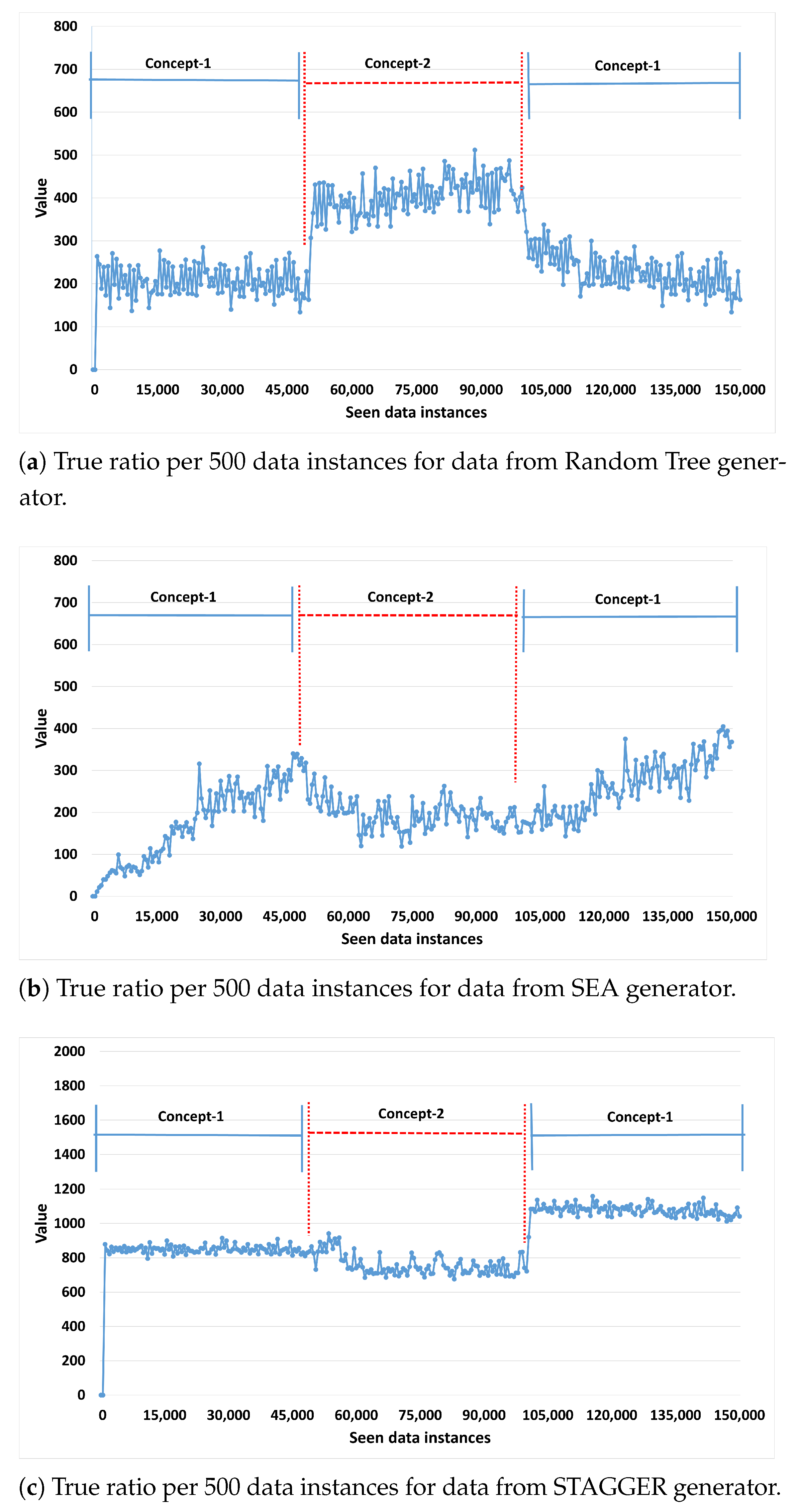
Concept Drift is likely and often unpredictable in non-stationary environments. The concept of the underlying data may change unpredictably at any time. Therefore, a streaming algorithm needs to be robust and have the ability to detect concept drift rapidly and effectively without expectation of any input from the user. This section aims to showcase the ability of FGRI to detect as well as adapt to new concepts in real-time autonomously. Figure 7a–c show evidence of the capability of FGRI to detect concept drift on the synthetic data streams. The reason why synthetic data stream generators have been used extensively is that they enable the induction of a concept drift deliberately and thus differently compared with real data streams, and the ground truth is known for evaluation. In each data stream observed there are two concept drifts, Concept 1 exists from 0 to the 50,000th data instance, Concept 2 from the 50,001st instance-to-instance 100,000 and then Concept 1 re-occurs. Thus, in each case two concept drifts occur. To indicate if a concept was picked up the True Positive rate over the last 500 instances at any time is calculated and plotted in the figures. The True Positive rate ranges from 0 to 1 and indicates the correctness/validity of the learned rules, 0 indicating the model does not fit the pattern and 1 indicating a perfect fit. Here, the reason for the inclusion of a reoccurring concept is that the model induced may have a different quality of fit for different concepts, even when not presented with a concept drift. Thus, ideally, the algorithm should respond to a recurring concept by reverting to its previous quality fit for that concept.
In Figure 7, the true positive rate is always above 0, indicating that the rule-set always contains at least some correct and valid rules. Regarding the Random Tree concept drifts (see Figure 7a) it can be seen that the true positive rate is stable at first and then increases after the first concept drift to concept 2, indicating that the algorithm adapts the model and can find an even better fit for concept 1. After the second concept drift, concept 1 re-appears and the algorithm adapts very quickly to the original level of the true positive rate, this fast recovery could be explained by the algorithm retaining some valid rules from concept 1 aiding in recovery of the true positive rate.
In Figure 7b, the model is applied on the SEA data stream. Here the algorithm learns more slowly, concept 1 improves over time, after the first Concept Drift it deteriorates a little, this is because the rule-set does not fit concept 2 well anymore. Generally, the algorithm does not adapt as responsively to concept 2 as very well; it does tend to adapt which is indicated by the true positive rate levelling off. However, then after the re-appearance of concept 1, the algorithm adapts more quickly and even improves upon the first fit to concept 1. This can be explained by the algorithm retaining some of the relevant rules for concept 1 after the first drift, so it can draw on a base rule-set to improve faster.
With regard to the STAGGER data stream (see Figure 7c) it can be seen that the drift has only a small effect on the true positive rate, indicating the algorithm is able to adapt and absorb some of the effects of the concept drift. It also recovers quickly after the 2nd concept drift, again indicating a portion of the previously valid rules were kept during concept 2 aiding in a quick recovery and even improvement after the 2nd concept drift.
6. Conclusions
This paper has presented the FGRI algorithm for inducing and maintaining an expressive and descriptive rule-set from data streams. The algorithm is able to automatically and incrementally induce a rule-set from streaming raw data (comprising categorical and numerical measurements). FGRI can adapt incrementally its rule-set to changes of the pattern encoded in the stream, and thus is applicable in real-time. Algorithms that induce this type of rule-set (generalised rules) only exist for static batch environments, but not for dynamically changing environments where the pattern encoded into the data stream may change (concept drift), and the rule-set needs to be adapted on the fly. Such dynamic and automatically adapting rule-sets can be used to (i) monitor the state of systems; (ii) explain changes to the analyst in real-time; (iii) provide actionable information to the human analyst. There are many possible fields of application, such as in the chemical process industry, telecommunications, social media tracking, etc. Currently, there are no comparable methods to FGRI that are applicable on data streams. This paper has provided FGRI evaluation at three levels: (1) theoretically, (2) qualitatively and (3) empirically. With respect to (1), a theoretical complexity analysis has been carried out. Unfortunately it is not possible to determine an accurate average case, as the complexity is dependent on the pattern encoded in the stream, and in turn the rule-set induced. All components with the exception of the induction of new rule bodies were linear. It was not possible to determine an average complexity for the induction of rule bodies, but only for an unlikely worst case resulting in a quadratic time complexity.However, it was further discussed that the average case is more likely to be linear, as it is limited by the number of rules induced which set the cut-off point in FGRI. With respect to (2), FGRI was evaluated in terms of its expressiveness to real data streams. The experiments captured the true positive and false positive ratios and absolute true positive and false positive values over time. The results showed that the rules induced were expressive, not random, and improved their expressiveness over time. In addition, regarding expressiveness, the rule-sets induced using the real datasets have been evaluated qualitatively and appear to reflect the concepts encoded in the stream correctly. FGRI was applied to two well-known datasets, treated as a stream, to qualitatively evaluate if the rules induced were plausible and matched the known relationships in the data. The rules induced reflected the knowledge available about the data, and thus it was concluded that FGRI enables the induction of meaningful and expressive rule-sets. With respect to (3), it was evaluated if FGRI can adapt its rule-set in real time to concept drift. For this, several data streams with known concept drifts were used, and the true positive rate over the rule-set over time was measured. In all cases FGRI successfully adapted to concept drift and successfully recovered.
Overall, the FGRI method constitutes a new kind of tool (data mining algorithm) in the Data Stream Mining toolbox and is as such complete. However, there are some limitations for which potential improvements as extensions to FGRI could be conducted in future research, As such, the induced rule-set is currently limited to 200 rules as this has been found to be consistent with the human cognitive-load-limit in terms of the number of rules a human can meaningfully handle for judgement and decision making in given context [76]. Yet a larger number of rules may be desired to capture more facets of the current concept in the data stream. For this, a possible research extension could be a layered dashboard that presents a contextualised and consolidated view of the rule-set. Furthermore, currently rules are limited to a maximum number of rule terms in order to avoid overfitting. Here a dynamic online-pruning method tailored for FGRI could be devised to improve rule quality further. Specific pointers and ideas in this direction are provided in Section 3.5. Although FGRI can handle both numeric and categorical data streams, it has been designed to be applied on tabular (symbolic) data streams and as such is not suitable for image data streams at sub-symbolic level. Extensions of FGRI towards image data streams are outside the scope of this project as these would require the prior establishment of the relevant human perceptual units of analysis and cognitive interpretation of sub-symbolic to symbolic structural labelling of semantic constituents of each image data frame.
Author Contributions
Conceptualisation, F.S.; Methodology, F.S., and T.L.; Software, T.L.; Validation, F.S., T.L., A.B., M.M.G.; Formal Analysis, T.L., F.S.; Visualization, F.S., T.L., A.B., M.M.G.; Investigation, F.S., T.L.; Resources, F.S.; Data Curation, T.L.; Writing Original Draft Preparation, F.S., T.L., A.B., M.M.G.; Writing Review Editing, F.S., A.B., M.M.G.; Supervision, F.S.; Project Administration, F.S.; Funding Acquisition, F.S. All authors have read and agreed to the published version of the manuscript.
Funding
This research has been supported by the UK Engineering and Physical Sciences Research Council (EPSRC) grant EP/M016870/1.
Institutional Review Board Statement
Not applicable.
Informed Consent Statement
Not applicable.
Conflicts of Interest
The authors declare no conflict of interest.
References
- Borgelt, C. Frequent item set mining. Wiley Interdiscip. Rev. Data Min. Knowl. Discov. 2012, 2, 437–456. [Google Scholar] [CrossRef]
- Liu, B.; Hsu, W.; Ma, Y.; Ma, B. Integrating Classification and Association Rule Mining. In Proceedings of the Fourth International Conference on Knowledge Discovery and Data Mining, New York, NY, USA, 27–31 August 1998. [Google Scholar]
- Agrawal, R.; Mannila, H.; Srikant, R.; Toivonen, H.; Verkamo, A.I. Fast Discovery of Association Rules. Adv. Knowl. Discov. Data Min. 1996, 12, 307–328. [Google Scholar]
- Wrench, C.; Stahl, F.; Fatta, G.D.; Karthikeyan, V.; Nauck, D. A Rule Induction Approach to Forecasting Critical Alarms in a Telecommunication Network. In Proceedings of the 2019 International Conference on Data Mining Workshops (ICDMW), Beijing, China, 8–11 November 2019; pp. 480–489. [Google Scholar]
- Nixon, M.J.; Blevins, T.; Christensen, D.D.; Muston, P.R.; Beoughter, K. Big Data in Process Control Systems. U.S. Patent App 15/398,882, 31 January 2017. [Google Scholar]
- Aggarwal, C. Data Streams: Models and Algorithms; Springer Science & Business Media: New York, NY, USA, 2007. [Google Scholar]
- Noyes, D. The Top 20 Valuable Facebook Statistics-Updated February 2014. 2014. Available online: https://zephoria.com/social-media/top-15-valuable-facebook-statistics (accessed on 6 January 2021).
- De Francisci Morales, G.; Bifet, A.; Khan, L.; Gama, J.; Fan, W. IoT Big Data Stream Mining. In Proceedings of the 22nd ACM SIGKDD International Conference on Knowledge Discovery and Data Mining-KDD ’16, San Francisco, CA, USA, 13–17 August 2016. [Google Scholar] [CrossRef] [Green Version]
- Motwani, R.; Babcock, B.; Babu, S.; Datar, M.; Widom, J. Models and issues in data stream systems. Invit. Talk. PODS 2002, 10, 543613–543615. [Google Scholar]
- Han, J.; Pei, J.; Kamber, M. Data Mining: Concepts and Techniques; Elsevier: Amsterdam, The Netherlands, 2011. [Google Scholar]
- Jin, R.; Agrawal, G. An algorithm for in-core frequent itemset mining on streaming data. In Proceedings of the Fifth IEEE International Conference on Data Mining (ICDM’05), Houston, TX, USA, 27–30 November 2005. [Google Scholar]
- Youn, J.; Shim, J.; Lee, S.G. Efficient data stream clustering with sliding windows based on locality-sensitive hashing. IEEE Access 2018, 6, 63757–63776. [Google Scholar] [CrossRef]
- Ibrahim, S.S.; Pavithra, M.; Sivabalakrishnan, M. Pstree based associative classification of data stream mining. Int. J. Pure Appl. Math. 2017, 116, 57–65. [Google Scholar]
- Nam, H.; Yun, U.; Vo, B.; Truong, T.; Deng, Z.H.; Yoon, E. Efficient approach for damped window-based high utility pattern mining with list structure. IEEE Access 2020, 8, 50958–50968. [Google Scholar] [CrossRef]
- Yun, U.; Kim, D.; Yoon, E.; Fujita, H. Damped window based high average utility pattern mining over data streams. Knowl. Based Syst. 2018, 144, 188–205. [Google Scholar] [CrossRef]
- Li, S.; Zhou, X. An intrusion detection method based on damped window of data stream clustering. In Proceedings of the 2017 9th International Conference on Intelligent Human-Machine Systems and Cybernetics (IHMSC), Hangzhou, China, 26–27 August 2017; Volume 1, pp. 211–214. [Google Scholar]
- Bifet, A.; Gavalda, R. Learning from time-changing data with adaptive windowing. In Proceedings of the 2007 SIAM International Conference on Data Mining, Minneapolis, MN, USA, 26–28 April 2007; pp. 443–448. [Google Scholar]
- Le, T.; Stahl, F.; Gaber, M.M.; Gomes, J.B.; Di Fatta, G. On expressiveness and uncertainty awareness in rule-based classification for data streams. Neurocomputing 2017, 265, 127–141. [Google Scholar] [CrossRef]
- Floyd, S.L.A. Semi-Supervised Hybrid Windowing Ensembles for Learning from Evolving Streams. Ph.D. Thesis, Université d’Ottawa/University of Ottawa, Ottawa, ON, Canada, 2019. [Google Scholar]
- Yun, U.; Lee, G.; Yoon, E. Advanced approach of sliding window based erasable pattern mining with list structure of industrial fields. Inf. Sci. 2019, 494, 37–59. [Google Scholar] [CrossRef]
- Yun, U.; Lee, G.; Yoon, E. Efficient high utility pattern mining for establishing manufacturing plans with sliding window control. IEEE Trans. Ind. Electron. 2017, 64, 7239–7249. [Google Scholar] [CrossRef]
- Gama, J.; Medas, P.; Castillo, G.; Rodrigues, P. Learning with Drift Detection. Brazilian Symposium on Artificial Intelligence; Springer: Berlin/Heidelberg, Germany, 2004; pp. 286–295. [Google Scholar]
- Baena-Garcıa, M.; del Campo-Ávila, J.; Fidalgo, R.; Bifet, A.; Gavalda, R.; Morales-Bueno, R. Early drift detection method. In Proceedings of the Fourth International Workshop on Knowledge Discovery from Data Streams, Berlin, Germany, 18–22 September 2006; Volume 6, pp. 77–86. [Google Scholar]
- Hammoodi, M.S.; Stahl, F.; Badii, A. Real-time feature selection technique with concept drift detection using adaptive micro-clusters for data stream mining. Knowl. Based Syst. 2018, 161, 205–239. [Google Scholar] [CrossRef] [Green Version]
- De Mello, R.F.; Vaz, Y.; Grossi, C.H.; Bifet, A. On learning guarantees to unsupervised concept drift detection on data streams. Expert Syst. Appl. 2019, 117, 90–102. [Google Scholar] [CrossRef]
- Hulten, G.; Domingos, P. VFML–A Toolkit for Mining High-Speed Time-Changing Data Streams. Software Toolkit. 2003, p. 51. Available online: http://www.cs.washington.edu/dm/vfml (accessed on 6 January 2021).
- Domingos, P.; Hulten, G. Mining high-speed data streams. In Proceedings of the Sixth ACM SIGKDD International Conference on Knowledge Discovery and Data Mining-KDD ’00, Boston, MA, USA, 20–23 August 2000; pp. 71–80. [Google Scholar] [CrossRef]
- Hulten, G.; Spencer, L.; Domingos, P. Mining time-changing data streams. In Proceedings of the Seventh ACM SIGKDD International Conference on Knowledge Discovery and Data Mining, San Francisco, CA, USA, 26–29 August 2001; pp. 97–106. [Google Scholar]
- Gama, J.; Kosina, P. Learning decision rules from data streams. In Proceedings of the Sixth ACM SIGKDD International Conference on Knowledge Discovery and Data Mining, Boston, MA, USA, 20–23 August 2000. [Google Scholar]
- Cano, A.; Krawczyk, B. Evolving rule-based classifiers with genetic programming on GPUs for drifting data streams. Pattern Recognit. 2019, 87, 248–268. [Google Scholar] [CrossRef]
- Nagaraj, S.; Mohanraj, E. A novel fuzzy association rule for efficient data mining of ubiquitous real-time data. J. Ambient. Intell. Humaniz. Comput. 2020, 11, 4753–4763. [Google Scholar] [CrossRef]
- Leite, D.; Andonovski, G.; Skrjanc, I.; Gomide, F. Optimal rule-based granular systems from data streams. IEEE Trans. Fuzzy Syst. 2019, 28, 583–596. [Google Scholar] [CrossRef]
- Ghomeshi, H.; Gaber, M.M.; Kovalchuk, Y. EACD: Evolutionary adaptation to concept drifts in data streams. Data Min. Knowl. Discov. 2019, 33, 663–694. [Google Scholar] [CrossRef] [Green Version]
- Barddal, J.P.; Gomes, H.M.; Enembreck, F. SFNClassifier: A scale-free social network method to handle concept drift. In Proceedings of the 29th Annual ACM Symposium on Applied Computing, Gyeongju, Korea, 24–28 March 2014; pp. 786–791. [Google Scholar]
- Idrees, M.M.; Minku, L.L.; Stahl, F.; Badii, A. A heterogeneous online learning ensemble for non-stationary environments. Knowl. Based Syst. 2020, 188, 104983. [Google Scholar] [CrossRef]
- Aggarwal, C.C.; Philip, S.Y.; Han, J.; Wang, J. A framework for clustering evolving data streams. In Proceedings 2003 VLDB Conference; Elsevier: Amsterdam, The Netherlands, 2003; pp. 81–92. [Google Scholar]
- Cao, F.; Estert, M.; Qian, W.; Zhou, A. Density-based clustering over an evolving data stream with noise. In Proceedings of the 2006 SIAM International Conference on Data Mining, Bethesda, MD, USA, 20–22 April 2006; pp. 328–339. [Google Scholar]
- Kranen, P.; Assent, I.; Baldauf, C.; Seidl, T. The ClusTree: Indexing micro-clusters for anytime stream mining. Knowl. Inf. Syst. 2011, 29, 249–272. [Google Scholar] [CrossRef]
- Carnein, M.; Trautmann, H. evostream–evolutionary stream clustering utilizing idle times. Big Data Res. 2018, 14, 101–111. [Google Scholar] [CrossRef]
- Shao, J.; Tan, Y.; Gao, L.; Yang, Q.; Plant, C.; Assent, I. Synchronization-based clustering on evolving data stream. Inf. Sci. 2019, 501, 573–587. [Google Scholar] [CrossRef]
- Din, S.U.; Shao, J. Exploiting evolving micro-clusters for data stream classification with emerging class detection. Inf. Sci. 2020, 507, 404–420. [Google Scholar] [CrossRef]
- Adedoyin-Olowe, M.; Gaber, M.M.; Dancausa, C.M.; Stahl, F.; Gomes, J.B. A rule dynamics approach to event detection in twitter with its application to sports and politics. Expert Syst. Appl. 2016, 55, 351–360. [Google Scholar] [CrossRef] [Green Version]
- Hong, T.P.; Wu, J.M.T.; Li, Y.K.; Chen, C.H. Generalizing concept-drift patterns for fuzzy association rules. J. Netw. Intell. 2018, 3, 126–137. [Google Scholar]
- Tang, F.; Huang, D.T.J.; Koh, Y.S.; Fournier-Viger, P. Adaptive Self-Sufficient Itemset Miner for Transactional Data Streams. In Pacific Rim International Conference on Artificial Intelligence; Springer: Berlin/Heidelberg, Germany, 2019; pp. 419–430. [Google Scholar]
- Lobo, J.L.; Laña, I.; Del Ser, J.; Bilbao, M.N.; Kasabov, N. Evolving spiking neural networks for online learning over drifting data streams. Neural Netw. 2018, 108, 1–19. [Google Scholar] [CrossRef]
- Schliebs, S.; Kasabov, N. Evolving spiking neural network—A survey. Evol. Syst. 2013, 4, 87–98. [Google Scholar] [CrossRef] [Green Version]
- Rudin, C. Stop explaining black box machine learning models for high stakes decisions and use interpretable models instead. Nat. Mach. Intell. 2019, 1, 206–215. [Google Scholar] [CrossRef] [Green Version]
- Angelov, P.; Soares, E. Towards explainable deep neural networks (xDNN). Neural Netw. 2020, 130, 185–194. [Google Scholar] [CrossRef]
- Vaughan, J.; Sudjianto, A.; Brahimi, E.; Chen, J.; Nair, V.N. Explainable neural networks based on additive index models. arXiv 2018, arXiv:1806.01933. [Google Scholar]
- Zliobaite, I.; Bifet, A.; Gaber, M.; Gabrys, B. Next challenges for adaptive learning systems. SIGKDD Explor. 2012, 14, 48–55. [Google Scholar] [CrossRef] [Green Version]
- Fürnkranz, J.; Gamberger, D.; Lavrač, N. Foundations of Rule Learning; Springer: Berlin, Germany, 2003; p. 334. [Google Scholar] [CrossRef]
- Michalski, R.S. On the Quasi-Minimal Solution of the General Covering Problem. 1969. Available online: http://ebot.gmu.edu/bitstream/handle/1920/1507/69-02.pdf?sequence=2&isAllowed=y (accessed on 6 January 2021).
- Bagallo, G.; Haussler, D. Boolean feature discovery in empirical learning. Mach. Learn. 1990, 5, 71–99. [Google Scholar] [CrossRef]
- Altman, D.G.; Bland, J.M. Statistics notes: The normal distribution. BMJ 1995, 310, 298. [Google Scholar] [CrossRef] [PubMed] [Green Version]
- Elliott, A.C.; Woodward, W.A. Statistical Analysis Quick Reference Guidebook: With SPSS Example; SAGE Publications: Thousand Oaks, CA, USA, 2007. [Google Scholar] [CrossRef]
- Ribeiro, M.I. Gaussian Probability Density Functions: Properties Furthermore, Error Characterization; Institute for Systems and Robotics: Lisboa, Portugal, 2004. [Google Scholar]
- Bramer, M. An information-theoretic approach to the pre-pruning of classification rules. In International Conference on Intelligent Information Processing; Springer: Berlin/Heidelberg, Germany, 2002; pp. 201–212. [Google Scholar]
- Bifet, A.; Holmes, G.; Pfahringer, B.; Kranen, P.; Kremer, H.; Jansen, T.; Seidl, T. MOA: Massive Online Analysis, a Framework for Stream Classification and Clustering. 2010. Available online: ebot.gmu.edu/bitstream/handle/1920/1507/69-02.pdf?sequence=2&isAllowed=y (accessed on 6 January 2021).
- Muthukrishnan, S. Data Streams: Algorithms and Applications; Now Publishers Inc.: Hanover, MA, USA, 2005. [Google Scholar]
- Babcock, B.; Babu, S.; Datar, M.; Motwani, R.; Widom, J. Models and issues in data stream systems. In Proceedings of the Twenty-First ACM SIGMODSIGACTSIGART Symposium on Principles of Database Systems PODS 02, Madiso, WI, USA, 3–5 June 2002; pp. 1–16. [Google Scholar]
- Hoeffding, W. Probability inequalities for sums of bounded random variables. J. Am. Stat. Assoc. 1963, 58, 13–30. [Google Scholar] [CrossRef]
- Haussler, D. Decision theoretic generalizations of the PAC model for neural net and other learning applications. Inf. Comput. 1992, 100, 78–150. [Google Scholar] [CrossRef] [Green Version]
- Maron, O.; Moore, A. Hoeffding Races: Accelerating Model Selection Search for Classification and Function Approximation. In Proceedings of the Advances in Neural Information Processing Systems, Denver, CO, USA, 28 November–1 December 1994; pp. 59–66. [Google Scholar]
- Gama, J.; Sebastião, R.; Rodrigues, P.P. On evaluating stream learning algorithms. Mach. Learn. 2013, 90, 317–346. [Google Scholar] [CrossRef] [Green Version]
- Street, W.N.; Kim, Y. A streaming ensemble algorithm (SEA) for large-scale classification. In Proceedings of the Seventh ACM SIGKDD International Conference on Knowledge Discovery and Data Mining, San Francisco, CA, USA, 26–29 August 2001; Volume 4, pp. 377–382. [Google Scholar] [CrossRef]
- Bifet, A.; Holmes, G.; Pfahringer, B.; Kirkby, R.; Gavaldà, R. New ensemble methods for evolving data streams. In Proceedings of the 15th ACM SIGKDD International Conference on Knowledge Discovery and Data Mining, Paris, France, 28 June–1 July 2009; pp. 139–148. [Google Scholar]
- Stahl, F.; Gaber, M.M.; Salvador, M.M. eRules: A Modular Adaptive Classification Rule Learning Algorithm for Data Streams. In International Conference on Innovative Techniques and Applications of Artificial Intelligence; Bramer, M., Petridis, M., Eds.; Springer: London, UK, 2012; pp. 65–78. [Google Scholar]
- Widmer, G.; Kubat, M. Learning in the presence of concept drift and hidden contexts. Mach. Learn. 1996, 23, 69–101. [Google Scholar] [CrossRef] [Green Version]
- Narasimhamurthy, A.; Kuncheva, L.I. A Framework for Generating Data to Simulate Changing Environments. In Proceedings of the 25th IASTED International Multi-Conference: Artificial Intelligence and Applications, AIAP’07, Phuket, Thailand, 2–4 April 2007; pp. 384–389. [Google Scholar]
- Delany, S.J.; Cunningham, P.; Tsymbal, A. A Comparison of Ensemble and Case-Base Maintenance Techniques for Handling Concept Drift in Spam Filtering. In Proceedings of the FLAIRS Conference, Melbourne Beach, FL, USA, 11–13 May 2006; pp. 340–345. [Google Scholar]
- Kuncheva, L.I. Classifier ensembles for changing environments. In International Workshop on Multiple Classifier Systems; Springer: Berlin/Heidelberg, Germany, 2004; pp. 1–15. [Google Scholar]
- Ikonomovska, E.; Gama, J.; Džeroski, S. Learning model trees from evolving data streams. Data Min. Knowl. Discov. 2010, 23, 128–168. [Google Scholar] [CrossRef] [Green Version]
- Olave, M.; Rajkovic, V.; Bohanec, M. An application for admission in public school systems. Expert Syst. Public Adm. 1989, 1, 145–160. [Google Scholar]
- Su, L.; Liu, H.Y.; Song, Z.H. A new classification algorithm for data stream. IJ Mod. Educ. Comput. Sci. 2011, 4, 32–39. [Google Scholar] [CrossRef] [Green Version]
- Fürnkranz, J.; Flach, P.A. ROC n’ rule learning-Towards a better understanding of covering algorithms. Mach. Learn. 2005, 58, 39–77. [Google Scholar] [CrossRef]
- Hernando, A.; Villuendas, D.; Vesperinas, C.; Abad, M.; Plastino, A. Unravelling the size distribution of social groups with information theory in complex networks. Eur. Phys. J. B 2010, 76, 87–97. [Google Scholar] [CrossRef]
- Bohanec, M.; Rajkovič, V. DEX: An expert system shell for decision support. Sistemica 1990, 1, 145–157. [Google Scholar]
Figure 1.
Overview of Windowing approaches to induce data mining models from streamining data.

Figure 2.
Main processes of generalised rule induction.

Figure 3.
Gaussian distribution of a classification from a continuous feature.

Figure 4.
Sliding windows approach to induce rules from streaming data.

Figure 5.
Iterations to specialise an inducing rule.

Figure 6.
Relationships between and on the real datasets as the data streams in and FGRI adapts.

Figure 7.
True ratio per 500 data instances from artificial streams.

Publisher’s Note: MDPI stays neutral with regard to jurisdictional claims in published maps and institutional affiliations. |
© 2021 by the authors. Licensee MDPI, Basel, Switzerland. This article is an open access article distributed under the terms and conditions of the Creative Commons Attribution (CC BY) license (http://creativecommons.org/licenses/by/4.0/).
Share and Cite
MDPI and ACS Style
Stahl, F.; Le, T.; Badii, A.; Gaber, M.M. A Frequent Pattern Conjunction Heuristic for Rule Generation in Data Streams. Information 2021, 12, 24. https://0-doi-org.brum.beds.ac.uk/10.3390/info12010024
AMA Style
Stahl F, Le T, Badii A, Gaber MM. A Frequent Pattern Conjunction Heuristic for Rule Generation in Data Streams. Information. 2021; 12(1):24. https://0-doi-org.brum.beds.ac.uk/10.3390/info12010024
Chicago/Turabian StyleStahl, Frederic, Thien Le, Atta Badii, and Mohamed Medhat Gaber. 2021. "A Frequent Pattern Conjunction Heuristic for Rule Generation in Data Streams" Information 12, no. 1: 24. https://0-doi-org.brum.beds.ac.uk/10.3390/info12010024
Note that from the first issue of 2016, this journal uses article numbers instead of page numbers. See further details here.