
A Workflow for Synthetic Data Generation and Predictive Maintenance for Vibration Data


1
Department of Electrical and Electronics Engineering, Bilkent University, 06800 Ankara, Turkey
2
TEKNOPAR, 06378 Ankara, Turkey
3
SINTEF, 7465 Trondheim, Norway
*
Author to whom correspondence should be addressed.
Information 2021, 12(10), 386; https://0-doi-org.brum.beds.ac.uk/10.3390/info12100386
Submission received: 20 August 2021
/
Revised: 10 September 2021
/
Accepted: 13 September 2021
/
Published: 22 September 2021
(This article belongs to the Special Issue Cognitive Digital Twins: Challenges and Opportunities for Process and Manufacturing Industries)
Abstract
:Digital twins, virtual representations of real-life physical objects or processes, are becoming widely used in many different industrial sectors. One of the main uses of digital twins is predictive maintenance, and these technologies are being adapted to various new applications and datatypes in many industrial processes. The aim of this study was to propose a methodology to generate synthetic vibration data using a digital twin model and a predictive maintenance workflow, consisting of preprocessing, feature engineering, and classification model training, to classify faulty and healthy vibration data for state estimation. To assess the success of the proposed workflow, the mentioned steps were applied to a publicly available vibration dataset and the synthetic data from the digital twin, using five different state-of-the-art classification algorithms. For several of the classification algorithms, the accuracy result for the classification of healthy and faulty data achieved on the public dataset reached approximately 86%, and on the synthetic data, approximately 98%. These results showed the great potential for the proposed methodology, and future work in the area.
1. Introduction
With the accelerated utilization of machine learning techniques in the context of industrial processes, predictive maintenance (PdM) has become a prominent research interest [1,2]. In an industrial context, the main goal of PdM is to optimize the maintenance schedule by predicting failures in machineries and processes. Such a process will result in reductions in unplanned downtimes of machinery, and fatal breakdowns [1,2]. Unplanned downtime can result in substantial losses for companies. Thus, it is crucial to reduce system downtime for the manufacturing industry. PdM reduces unnecessary maintenance, which further increases the machine’s life, considering that every maintenance operation causes downtime [3]. Another advantage of PdM is cost minimization, including minimizing fatal breakdowns and reducing the replacement of key components, which is closely related to the previously mentioned benefits [4]. Predictive maintenance may reduce maintenance costs by 25–35%, eliminate downtimes by 70–75%, reduce downtime by 35–45%, and increase productivity by 25–35% [1,2].
Aivaliotis et al. [5] investigated PdM for manufacturing resources by utilizing physics-based simulation models and the Digital Twin (DT) concept. In large industrial sectors, DT’s capability to predict the future performance of processes is seen as highly valuable [6,7]. Werner et. al. [8] suggested a holistic PdM strategy, employing a hybrid approach combining data and physics-based modeling to estimate remaining useful life [8]. In addition, in [9,10], an assessment of the application of machine learning techniques and ontologies in the context of PdM reported the application areas such as fault diagnosis, fault prediction, anomaly detection, time to failure, and remaining useful life estimation, which refer to the various stages of PdM.
The number of publications on the application of machine learning for PdM has increased dramatically [11]. A major challenge in developing and implementing a PdM procedure based on machine learning is data quality; quality training data are essential when building an ML-based predictive maintenance pipeline. It is difficult to obtain failure data of sufficient quality and in sufficient quantity. This is particularly true when the machine is new and without historical data. This current work involves exploration of the generation of synthetic data from physics-based models to create failure data. Vibration is the mostly studied measurement for PdM in manufacturing Table 5 in [11].
This paper validates the proposed approach and demonstrates its application to the COGNITWIN project use case pilot on Spiral Welded Machinery (SWP) in the steel pipe industry. In this industry, machinery is generally very large-scale, thus making it difficult to track conditions and monitor health, which are crucial for product quality and process safety. Under the COGNITWIN project scope, the hybrid digital twin was developed for the production process of Spiral Welded Steel Pipe machinery (SWP). Improving the operational performance of the production process is targeted by predicting and identifying the optimal operating parameters, based on both historical and real-time data and first-order physical models.
Synthetic data generation for predictive maintenance purposes is a developing concept drawing attention from various industrial sectors; thus, there have been many recent studies in this topic. For instance, in [12], there was a discussion of several different data generation approaches for use in predictive maintenance, including synthetic data generation based on a virtual simulation model or based on a simplified real-life physical model. However, for data generation, the authors suggested using, rather than a digital twin, a real-life simplified physical model of the system from which they actively measure data with placed sensors. In contrast, in this study, the synthetic data generation was heavily dependent on the digital twin model of the motor and gearbox; the data are the output of the virtual simulations conducted on this model. Several studies have recommended using virtual models for synthetic data generation (such as [5,13]). Most studies on predictive maintenance (especially on vibration data) found in a literature search have explained predictive maintenance workflow conceptually, rather than explicitly describing the steps of the workflow. In this study, we presented a complete workflow for the application of predictive maintenance for vibration signals. Steps in the proposed workflow are specialized to vibration data but can also be used to experiment with signals that have similar periodic characteristics (needed because of the proposed extracted condition indicators that belong in the frequency domain) and transient responses (needed because of the proposed pre-processing step), such as sinusoidal electrical circuits. Studies that have integrated deep learning structures (such as RNNs and LSTMs) into data-driven prognostic methods include [14], which explored transfer learning for remaining useful life predictions, and [15], which proposed adaptive time-series prediction for prognostics of lithium-ion batteries. Unlike these two papers, deep learning structures were not implemented in this study, as it was experimentally determined that other state-of-the-art classification algorithms functioned with acceptable accuracy for the experiments. However, it should be noted that deep learning structures are also compatible with the proposed algorithm.
Overall, the main objective of this study was to propose a viable means of generating synthetic vibration data for healthy and faulty conditions and to create a viable methodology for predictive maintenance of these vibration signals. Although predictive maintenance and digital twin concepts have been investigated in many studies, very few specifically target vibration signals, and prior work on the subject has been found to be lacking details regarding the proposed algorithms. Thus, the proposal of a novel and complete workflow for periodic signals would be useful and beneficial for numerous areas of industry using such data, which reflects the essential motivation for this paper. The contributions of this paper can be listed as follows:
- A method for building a digital twin model (of a motor and gearbox circuit specifically in this study) and generating synthetic healthy and faulty data using this model is proposed.
- A predictive maintenance algorithm to estimate the current state of the machine/digital twin is presented for all types of periodic signal (vibration data specifically in this study), and steps of this algorithm are described in detail to ensure reproducibility. The proposed predictive maintenance algorithm can work with both synthetic data and suitable real-life data.
- A publicly accessible vibration dataset and digital twin model-generated synthetic data were used to test the classification accuracy of the proposed predictive maintenance algorithm, in terms of correctly classifying healthy and faulty data.
2. Methodology
The methodology of this study can be described under three main sections: creating the digital model, constructing the predictive maintenance workflow, and testing the predictive maintenance algorithm. In this section, the methodology of the study is explained.
2.1. Creating the Digital Twin Model
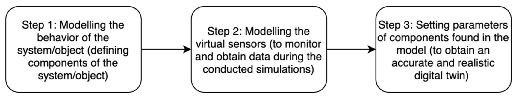
The first step in the methodology is creating the digital twin model for use throughout the study. In this step, the aim was to build a high-fidelity physical model of the real-life physical object or system under focus. The three main parts of this step are modeling the behavior of the individual components, modeling the behavior of the overall system (collection of components), and finally, modeling the sensors and fine-tuning the parameters [5], as shown in Figure 1 below.
The system modeled consists of a motor and gearbox. The circuit includes components from electrical, thermal, rotational motion, and translational motion domains. The system represents the motor circuit of the main driver of a metal sheet roller machine. Two main base components of the model are the universal (electrical and mechanical components) motor, driven by a DC voltage source, and the gearbox, which reduces the rotation of the motor. The DC-driven universal motor of the circuit is designed based on electrical (Kirchhoff’s voltage law) and mechanical (Newton’s second law of motion) equations. The two governing equations of the motor are (Kirchhoff’s voltage law), where is the input voltage, is the motor resistance, is the motor current, is the motor inductance, and is the back electromotive force, and (Newton’s law), where is the electromotive torque, is the load torque, is the total inertia, is the angular velocity, and is the angular friction. The two equations are connected by the relationship between electromotive force and angular velocity (, where is the back electromotive force constant), as well the relationship between the torque and current (, where is the torque constant). Figure 2 below shows a simple physics-based schematic of a DC-driven universal motor [16].
However, as stated, this study was focused on investigating the vibration signals. Thus, one of the key parts of the model is the vibration signal created by the subsystem that transforms the total rotational displacement at the output of the motor and gearbox to translational motion via masses and springs. The vibration signal is measured from the spring-damper chain found in this subsystem. The thermal domain components are temperature sensors, which can monitor the heat exchange between the motor and the environment. All measurements are gathered by respective sensors placed in the model (electrical sensors, thermal sensors, translational motion sensors, and rotational motion sensors). The main technical challenge in the model creation step was obtaining a reliable and accurate vibration output signal compatible with the digital twin model. With the initial version of the twin model, adding a subsystem that directly generates a vibration signal failed to yield desired results due to the operation mechanisms of the existing fault models. To ensure a satisfactory vibration output, the digital model was renovated, and several obsolete fault models and sensors were removed and replaced by new fault subsystems, as well as a subsystem to generate a vibration signal, creating more accurate vibrations from the digital twin. Another challenge was to find a suitable consistency tolerance for the solver configuration of the model. The default value for the consistency tolerance () provided by Simulink caused some simulations to raise error flags, and the interruption of the whole simulation process, due to calculational insensitivities of the motor current signals. This consistency tolerance was alleviated to to eliminate false error flags and obtain a smoother simulation process. The digital twin model was constructed in MATLAB Simulink, and all simulations/data generation and gathering related to the twin model were carried out in MATLAB. Figure 3 below shows the digital twin model created in MATLAB Simulink.
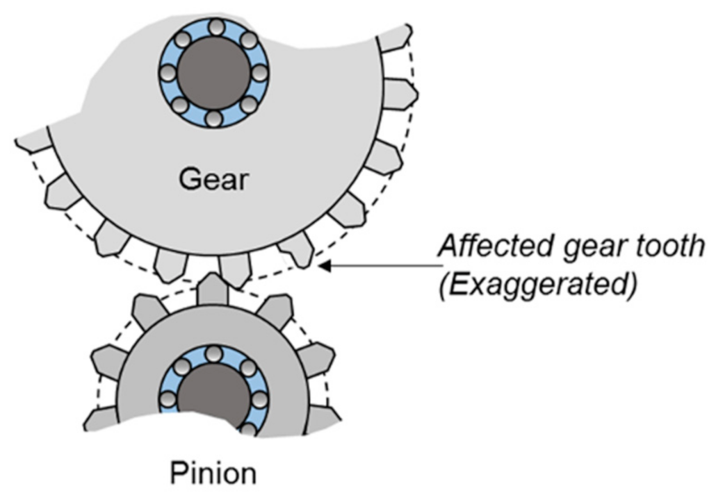
Fault modeling is a key part of a digital twin model used in predictive maintenance [17]. In this study, the main emphasis of the model was also the fault modeling. Two fault types were investigated and modeled in this study: gearbox tooth faults and vibration sensor errors. The tooth fault was modeled by inserting an undesired faulty torque at a fixed position (an error in a fixed tooth) in the turn of the gearbox shaft. A value of this disturbance torque of 0I indicates no error in the model. A visualization for gearbox tooth faults is shown in Figure 4. The second type of error source is in vibration sensors. In order to represent both the measurement errors and the intrinsic mechanical errors of these sensors, a simple offset was inflicted in the measurement of the vibration sensors; a value of 0 in this offset indicates no error in the measurement of vibration signals.
Both errors (gearbox tooth fault and vibration sensor drift) described in the previous paragraph are modeled as subsystems in the diagram shown in Figure 3 above. Another subsystem shown in the diagram functions as a tachometer, in case it was needed. Although this subsystem was not used in this study, it is potentially valuable in further work. The tachometer’s output (output of the subsystem) contains pulses that correspond to the rotations of the motor and the gearbox.
The content of the digital physics-based model is as explained above. The last part of the modeling step is setting the parameters of the components of the twin, as shown in Figure 1 above. For this part, the parameters of the components were carefully tuned and set, after consulting the owner of the SPW machinery, the firm NOKSEL. To create conditions that were as close to reality as possible, all the parameters were set to the values provided by the owning firm, and if the exact value of a parameter could not be obtained, an approximation was made that was known to be correct to the nearest order of magnitude. As can be seen from Figure 3 above, the digital twin model contains 87 components, and in consequence, many parameters. These parameters include the electrical power, inertia and rated speed of the universal DC motor, voltage of the DC supply that drives the motor, follower-to-base teeth ratio of the gearbox, resulting losses of the system due to friction, and values of masses and inertias in the damping components. As can be understood from this variety of components, for the purpose of the digital twin, it is crucial to be as close to the real values of parameters as possible. If the parameters of components are unrealistic, the behavior and the output signals of the digital twin would not reflect the actual behavior of the SPW machinery. Thus, a precise co-operation was conducted with NOKSEL to fine-tune the component parameters. After the parameter calibration step, the modeling was completed. The main benefit of a physics-based digital twin model is the ability to generate synthetic data. In this study, the described digital twin model was constantly used to generate both healthy and faulty synthetic data, for use in the later stages, during the predictive maintenance algorithms development.
2.2. Predictive Maintenance Workflow
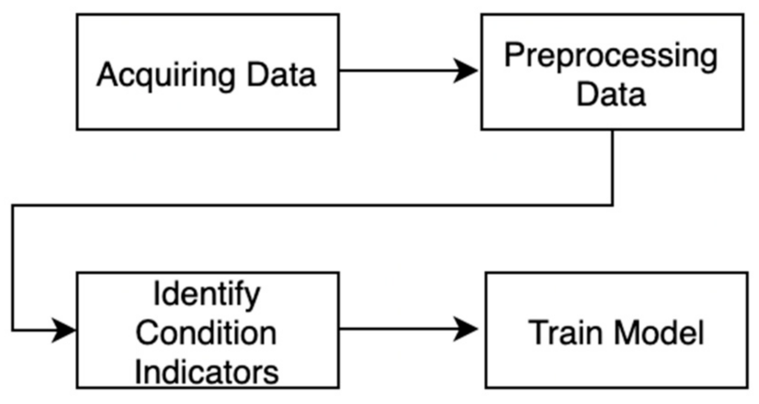
In general, a basic predictive maintenance workflow has four main steps [19]: data acquisition, preprocessing, identifying condition indicators, and training. An image depicting these four steps can be seen in Figure 5 below.
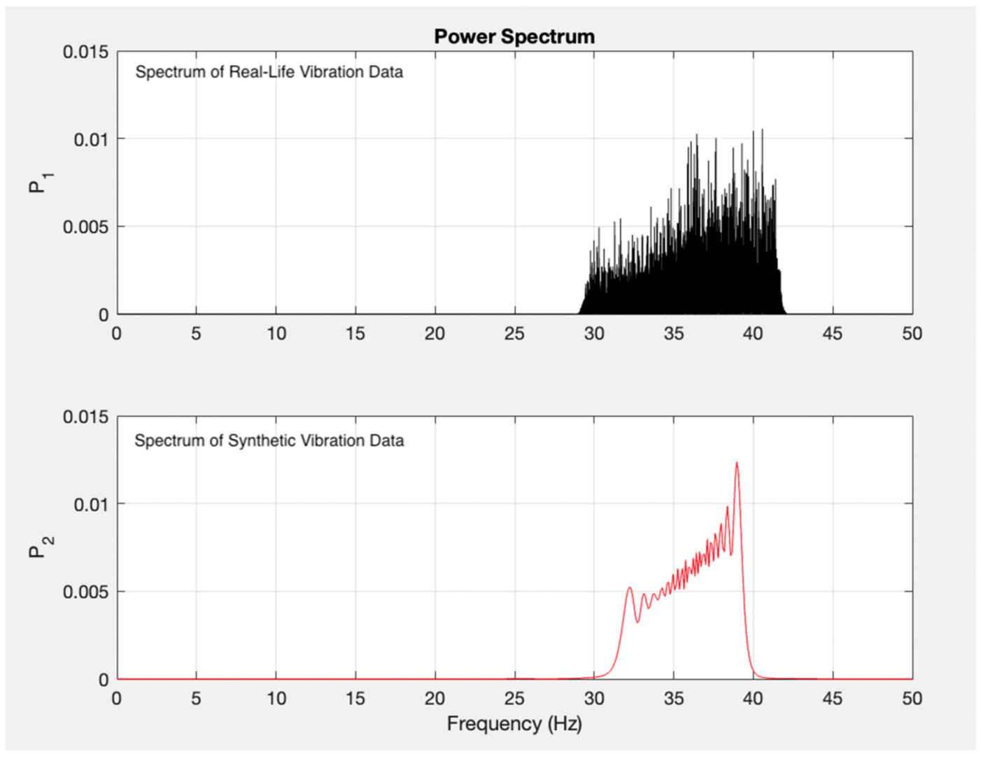
As shown in Figure 5, the first step of the algorithm is acquiring the data to be worked on. Each predictive maintenance workflow begins with data, either synthetic or real-life data [12]. In this study, synthetic data were generated via the digital twin model described in the previous subsection. The digital twin model is configured with error variables that describe the level of two error sources, namely gearbox tooth fault and sensor errors, as explained above. Changes in the values of these error variables in different simulation runs generate different vibration data. In order to ensure generalizability of the results, the values of error variables were assigned randomly in different simulations from a certain boundary of values. The synthetic data generation algorithm is briefly described in Algorithm 1 below. As well as the synthetic data, real life data were also used to test the created predictive maintenance algorithm (the testing process is explained in detail in the following section). Real life vibration data were acquired with a sampling period of 10 ms and the data included 411,863 datapoints. Furthermore, a frequency domain analysis was carried out to confirm the resemblance between the generated synthetic data and measured real-life data. Both real-life and synthetic data were transformed via the Fourier transform, and frequency contents were compared via power spectra and peak frequency analysis. The resulting graph of the power spectra analysis, shown in Figure 6 below reveals that the bandwidth of the synthetic data (spectrum shown in the bottom graph in Figure 6) and the bandwidth of the real-life vibration data (spectrum shown in the top graph in Figure 6) were both between approximately 30 and 45 Hz, and the peak frequencies were at approximately 39 Hz in both data. The boundary of power values for each data was also very close, indicated by the y-axis of both graphs in Figure 6.
| Algorithm 1 Synthetic Data Generation Algorithm |
| Input: Description of the List of Failures |
| (1) Develop Detailed Physics-Based Model of the Process |
| (2) Develop and Implement Modelling Strategies of the Failures |
| (3) Input Realistic Range of Variables Responsible of the Failures |
| Randomly vary the Variables Responsible of the Failures |
| Run Until Enough Data |
| Output: Supervised Dataset for Predictive Maintenance |
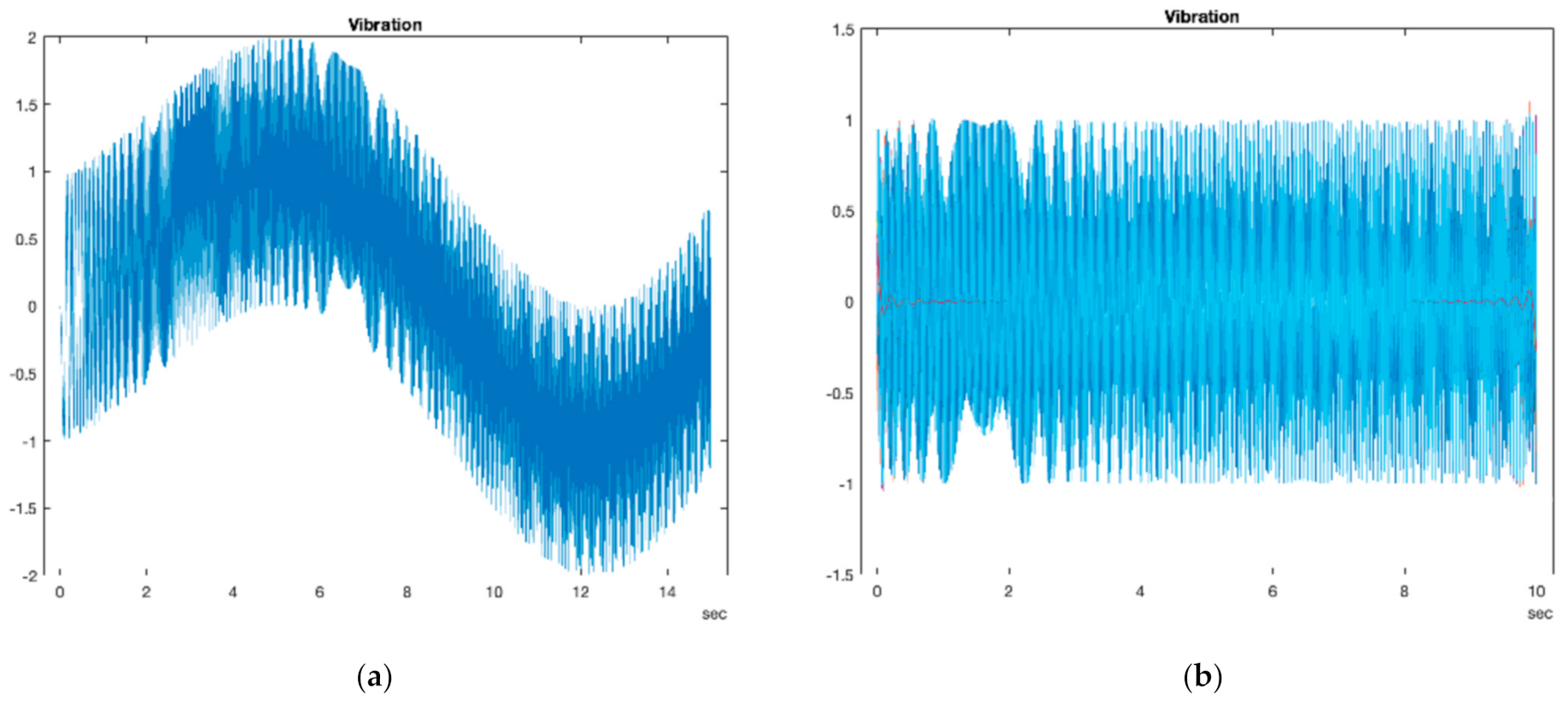
The next step of the predictive maintenance workflow is preprocessing. Preprocessing is essential for all applications of machine learning model development processes in the following step, extracting condition indicators [20]. In this step, the raw data are manipulated and transformed into a form that facilitates the extraction of features and indicators. In this study, the preprocessing step consisted of three sub-steps. First, the first section of simulation outputs, called the transient response of the simulation, was removed to obtain the actual frequency contents of the signal. Then, the signals were filtered to reduce the noise. Lastly, in this step, each simulation was classified based on the type of error. There are two different error variables, and either of these may or may not induce an error based on its value; thus, four different classes emerge. If both error variables are in the boundary, such that they induce no error, the simulation is said to be in the healthy condition (Class 0), and if both error variables are in the error interval, the simulation is said to be in Class 3 (both variables induce error). In Class 1, there is only a gearbox tooth fault present in the simulation, and in Class 2, only vibration sensor drift error. Another challenge in the synthetic data generation process was determining the threshold levels for the error source variables, which indicates whether a simulation condition is healthy or faulty. As the values for the error variables were randomly given from a specified interval, choosing very small healthy condition boundaries resulted in domination of the sampling of faulty conditions, lowering the accuracy of identification of the healthy conditions in the classifier model training step, because the healthy condition class was under-sampled. Such a sampling inequality was overcome by broadening the threshold values specifying the healthy conditions, leading to a greater overall accuracy of the classifier. Figure 7 below shows an example simulation output before the preprocessing step (Figure 7a) and after (Figure 7b). Note that the first 5 s of the signal (the initial transient response) in Figure 7a was removed, as well as the noise.
The following step was the identification of the condition indicators, also called features. Features are properties belonging to a particular dataset that change in an anticipated manner as the system itself changes or deteriorates [21]. Condition indicators are features involved in many different areas of signal analysis, including time domain features (e.g., mean and standard deviation), frequency domain features (e.g., power bandwidth and peak frequency), and time–frequency domain features (e.g., special entropy and special kurtosis). In this study, the following 18 different features from time and frequency domains were extracted from the preprocessed data: signal mean, median, RMS value, variance, peak value, peak-to-peak value, skewness, kurtosis, crest factor, median absolute deviation (MAD), range of cumulative sum, correlation dimension, approximate entropy, Lyapunov exponent, peak frequency, high-frequency power, envelope power, and spectral kurtosis. As seen, the features used belong to the time domain, frequency domain, and time–frequency domain. These features were chosen as being well-established types of evaluating signal data, in particular, signals that have distinct frequency content, as in the case of vibration signals [22]. After all 18 features were extracted from the data, neighborhood component analysis (NCA) was applied to the features for the two error sources in the model. NCA ensures that only relevant features (relevant condition indicators) are retained and that the others (those not useful in diversifying different error classes) are disregarded. This accelerates the final step of the predictive maintenance workflow, model training.
Model training is the final step of the predictive maintenance workflow of this study, as mentioned above. A trained model lies at the heart of the predictive maintenance algorithm. This model examines extracted condition indicators (or features), either to assess the system’s present state (fault detection and diagnosis) or to forecast its future state (remaining useful life prediction). After the features are extracted from the preprocessed data, and NCA is used to disregard undecisive features, and the remaining features are used to train a machine-learning model to determine the current error condition of the physics-based model. In both synthetic data and public dataset cases, the remaining features were the same, and for both cases, NCA decreased the number of features from 18 to 11: mean, median, peak, kurtosis, crest factor, MAD, range of cumulative sum, correlation dimension, approximate entropy, Lyapunov exponent, and envelope power. Determining the current condition of the digital twin model means assigning a class of error conditions to the current state of the model (according to current value of error variables) among the four error condition classes described earlier. Details of the model training are explained in the following subsection.
2.3. Testing the Predictive Maintenance Algorithm
The proposed predictive maintenance workflow described in the previous subsection was tested by two methods. The first test used bearing data provided by the public dataset of Case Western Reserve University (CWRU) [23,24]. This dataset provides bearing test data for normal and faulty bearings, which resembles the results aimed at by generating synthetic data (healthy and faulty conditions). As with the synthetic data, the CWRU data also included four classes, one healthy and three faulty. Data in the public dataset were collected at 12,000 samples per second. These collections were continuous measurements, and in different time intervals, different fault conditions were exposed. However, in order to create enough different data elements, the continuous measurements were segmented by 1001 data points (in order to accord with the synthetic data, which consisted of 1001 data points for different simulations, as explained subsequently). In order to test the proposed predictive maintenance algorithm, the dataset was first preprocessed as explained in the previous subsection. Then, the features listed in Section 2.2 were extracted from the preprocessed data, and NCA was applied to eliminate unhelpful features. The process concluded with the training of the diagnosis model (the model that estimates the current state of the digital twin). This training involved the feature table composed of all 11 relevant features remaining after NCA, as listed in the previous section, for all data elements. Then, this feature table was used for training with many different state-of-art machine learning algorithms, such as SVM, ensemble trees, naïve Bayesian, KNN, and discriminant methods. The accuracy of these predictions was examined with different algorithms to assess the success of the proposed predictive maintenance algorithm. Of the many classification algorithms that were used to train the model, the 5 above-listed algorithms yielded the most accurate results for both the synthetic data and the public CWRU dataset during classification. Thus, the classification accuracy for these 5 algorithms is presented in the graphs and discussed in the next section, Results and Discussion.
The second test of the algorithm was conducted on the generated synthetic data. This test resembles the test with the public CWRU dataset but using the synthetic data from the digital twin model instead of the bearing data from the public dataset. These synthetic data were also a continuous measurement for each simulation. Each simulation was run with different error variable values and lasted 15 s. In the preprocessing, the first 5 s was removed as the transient response, leaving 1001 measurements (1001 data points) in each simulation. For each error variable, 50 random variables were used; thus, in total, simulations were obtained, which means 2500 different elements were classified in the training model. The number of random variables (50) was deliberately chosen for computational efficiency, a priority in this study. In addition, 2500 simulations yielded a large enough dataset to run classification models, without producing very complex and time-consuming results. If computational efficiency had not been a concern, the number of different error variables could be increased, as discussed in the future work section. Once again, the features listed in Section 2.2. were extracted from the data, and NCA was applied to eliminate unhelpful features. The resulting feature table (with the remaining 11 features listed above in Section 2.2, as with the CWRU dataset case) was used in training with the same algorithms as listed in the previous paragraph, and once again, the accuracies of these predictions were examined to deduce the accuracy of the proposed algorithm. The overall, complete flowchart of the proposed workflow, including the synthetic data generation step, is shown in Figure 8 below. The classification accuracy results for the CWRU dataset and synthetic data are presented and discussed in the following section.
3. Results and Discussion
This section contains a discussion of the results of the classification accuracy after model training for the CWRU dataset and the synthetic data. First, Figure 9 below, showing the accuracies for the CWRU, reveals that, regardless of which algorithm is used to train the diagnosis model, the estimation of the current state of the system was better than chance. The best-performing algorithm was the ensemble bagged tree, with the accuracy of 85.85%. The yields in accuracy in classification were as follows: weighted KNN, 73.76%; cubic SVM, 67.82%; quadratic discriminant, 59.72%; and naïve Bayesian, 56.94%. The better-than-chance training accuracy for each algorithm, and the models’ ability to estimate the current state of the system with over 70% accuracy for some algorithms, showed that the algorithm works as desired for the CWRU dataset. In Figure 10, the accuracy results for the synthetic data are shown. Notice that the limits of the y-axis in Figure 10 are different than those in Figure 9.
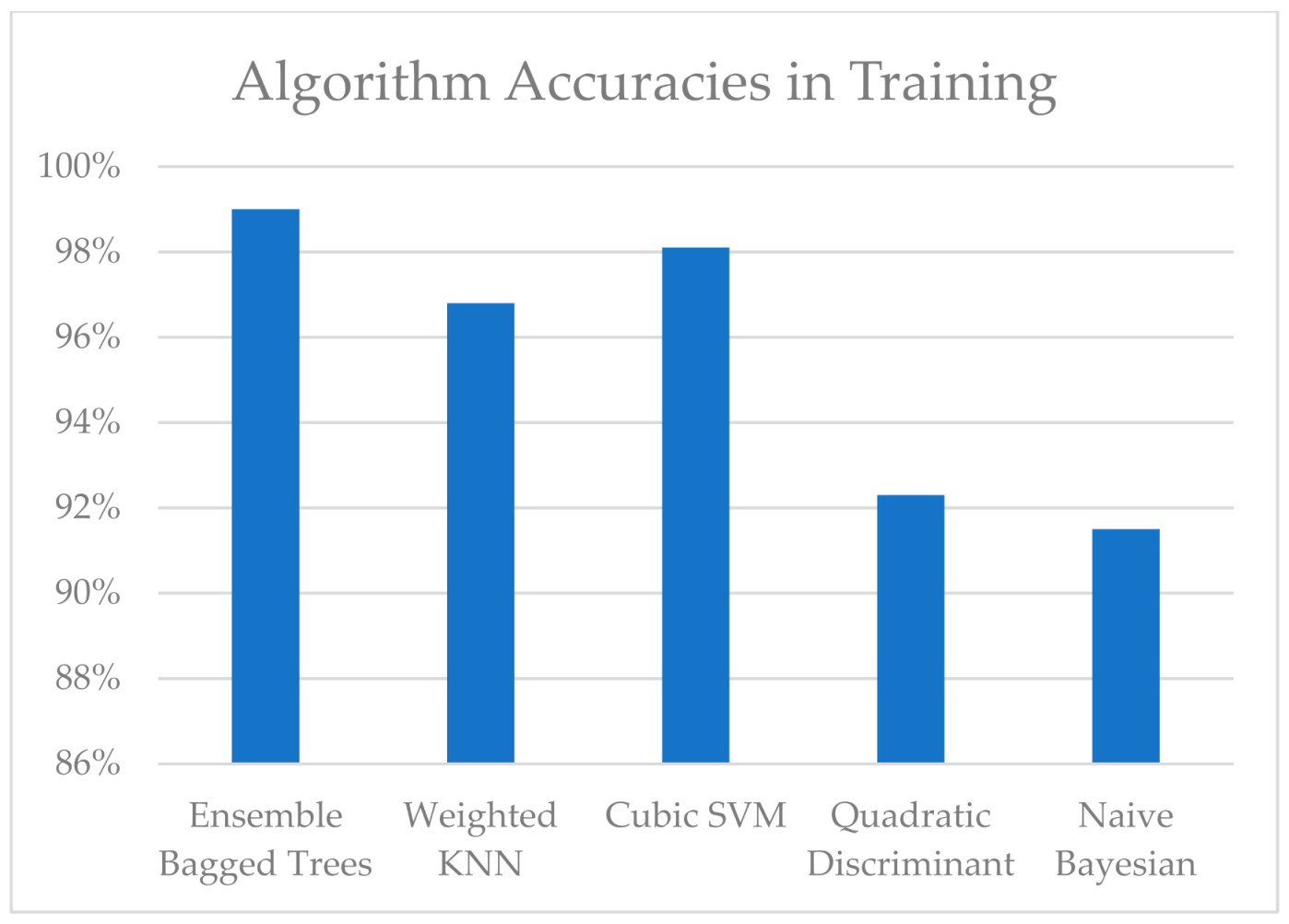
As can be seen from Figure 10, for all algorithms, the accuracy of state estimation was greater than 90%. The highest accuracy was once again with ensemble bagged trees, at 99%. The accuracies for cubic SVM, weighted KNN, quadratic discriminant, and naïve Bayesian were 99%, 98.1%, 96.8%, 92.3%, and 91.5%, respectively. It can be deduced that the proposed predictive maintenance algorithm worked exceptionally well for the synthetic data. However, there was a clear performance difference between the synthetic data and CWRU dataset because the measurements in the CWRU dataset were taken from a real-life device, making it practically impossible to obtain the same measurements and characteristics for a certain error class at different times. However, synthetic data generation is a theoretical process, and the characteristics of an error class can be exactly replicated in different runs. Thus, the classification gives very accurate results for synthetic data, as the characteristics for different classes can be exactly replicated for different elements in a particular class.
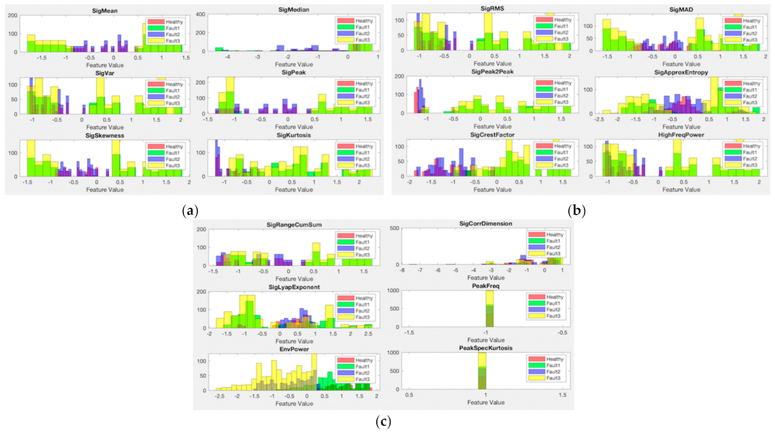
In Figure 11 below, feature vs. classes histograms for the classification in the synthetic data case with the ensemble bagged tree algorithm are shown, where, in each graph, the y-axis corresponds to the number of datapoints. Graphs in Figure 11 show the feature vs. class diagrams for each feature (before applying NCA and eliminating features) for the synthetic data. It can clearly be seen that peak spectral kurtosis (shown on the bottom right in Figure 11c) is an irrelevant feature for classifying the different faulty conditions, as it is unable to separate different classes, and will likely be eliminated through applying NCA. On the other hand, Figure 11b shows that approximate entropy is a good feature to separate healthy conditions from faulty conditions and will likely be used as a feature in the classification model. Figure 10 clearly demonstrates that some features can easily differentiate between different classes, and through multiple features, the trained model can classify different error conditions and estimate the current system state with very high accuracy.
4. Conclusions
The main goal of this study was to suggest a viable workflow to generate healthy and faulty synthetic vibration data, and to bring forward a feasible predictive maintenance algorithm to classify these faulty and healthy data. This main objective was met by a process involving creating an algorithm consisting of a digital twin model of the system, generating the synthetic data, preprocessing the synthetic data, and extracting condition indicators (also called features) from the preprocessed data and machine learning model training. The success of this proposed methodology was assessed through two test processes. First, the proposed methodology was applied to the CWRU public-bearing dataset, and the success of the workflow in classifying the faulty conditions was better than chance for five different state-of-the-art machine learning algorithms. For some of these algorithms, the classifying accuracy reached approximately 85%. Secondly, the proposed methodology was tested on the synthetic data generated by the digital twin model. For the synthetic data, the workflow was very successful in classifying different simulation conditions (different faults), with the accuracy of classifications above 90% for the same five ML algorithms, and in some cases, reaching approximately 99%. These results showed that the proposed methodology functions as desired, with acceptable accuracy in classification.
The scope of the future work in this area should consider several key aspects. One of these is the size of the synthetic data dataset. In this study, two error variables were used to generate 2500 unique simulations and the classification accuracy was very high. In order to further test the proposed methodology, more error variables may be used in the digital twin model, to obtain more than 2500 unique simulations. It should be remembered, however, that this would increase the computational cost and decrease the time-efficiency of the study. Furthermore, the digital twin model used in the study may be upgraded to a cognitive twin model, and also state estimation filters, such as Kalman filtering, may be used to update the component parameters to obtain more realistic data from the physics-based model. In summary, the proposed methodology was successful in creating faulty and healthy synthetic data, and in classifying the faulty conditions within the desired boundaries.
Author Contributions
Conceptualization, Ş.Y.S., M.J. and P.Ü.; introduction, P.Ü. and Ö.A.; methodology, Ş.Y.S. and M.J.; validation, M.J. and P.Ü.; formal analysis, Ş.Y.S.; investigation, Ş.Y.S.; writing—original draft preparation, Ş.Y.S.; writing—review and editing, Ş.Y.S., P.Ü., Ö.A. and M.J.; visualization, Ş.Y.S.; supervision, M.J. and P.Ü.; project administration. All authors have read and agreed to the published version of the manuscript.
Funding
This research was funded by the European Union’s Horizon 2020 research and innovation programme, under grant number 870130 (the COGNITWIN project).
Data Availability Statement
Case Western Reserve University’s fault test data were analyzed in this study. This data can be found here: https://engineering.case.edu/bearingdatacenter. The generated synthetic data from the digital twin model are not publicly available due to privacy.
Acknowledgments
The authors thank TEKNOPAR for its administrative and technical support.
Conflicts of Interest
The authors declare no conflict of interest.
References
- Krupitzer, C.; Wagenhals, T.; Züfle, M.; Lesch, V.; Schäfer, D.; Mozaffarin, A.; Edinger, J.; Becker, C.; Kounev, S. A survey on predictive maintenance for industry 4.0. arXiv 2020, arXiv:2002.08224. [Google Scholar]
- Jimenez, J.J.M.; Schwartz, S.; Vingerhoeds, R.; Grabot, B.; Salaün, M. Towards multi-model approaches to predictive maintenance: A systematic literature survey on diagnostics and prognostics. J. Manuf. Syst. 2020, 56, 539–557. [Google Scholar] [CrossRef]
- Baidya, R.; Ghosh, S.K. Model for a Predictive Maintenance System Effectiveness Using the Analytical Hierarchy Process as Analytical Tool. IFAC-PapersOnLine 2015, 48, 1463–1468, ISSN 2405-8963. [Google Scholar] [CrossRef]
- Deloux, E.; Castanier, B.; Bérenguer, C. Predictive maintenance policy for a gradually deteriorating system subject to stress. Reliab. Eng. Syst. Saf. 2009, 94, 418–431. [Google Scholar] [CrossRef] [Green Version]
- Aivaliotis, P.; Georgoulias, K.; Chryssolouris, G. The Use of Digital Twin for Predictive Maintenance in Manufacturing. Int. J. Comput. Integr. Manuf. 2019, 32, 1067–1080. Available online: https://www.researchgate.net/profile/Luca-Romeo-2/publication/327334242_Machine_Learning_approach_for_Predictive_Maintenance_in_Industry_40/links/5e15db8792851c8364badb48/Machine-Learning-approach-for-Predictive-Maintenance-in-Industry-40.pdf (accessed on 3 August 2021). [CrossRef]
- Melesse, T.Y.; Di Pasquale, V.; Riemma, S. Digital Twin models in industrial operations: State-of-the-art and future research directions. IET Collab. Intell. Manuf. 2021, 3, 37–47. [Google Scholar] [CrossRef]
- Liu, M.; Fang, S.; Dong, H.; Xu, C. Review of digital twin about concepts, technologies, and industrial applications. J. Manuf. Syst. 2021, 58, 346–361. [Google Scholar] [CrossRef]
- Werner, A.; Zimmermann, N.; Lentes, J. Approach for a holistic predictive maintenance strategy by incorporating a digital twin. Procedia Manuf. 2019, 39, 1743–1751. [Google Scholar] [CrossRef]
- Melesse, T.Y.; Di Pasquale, V.; Riemma, S. Digital twin models in industrial operations: A systematic literature review. Procedia Manuf. 2020, 42, 267–272. [Google Scholar] [CrossRef]
- Dalzochio, J.; Kunst, R.; Pignaton, E.; Binotto, A.; Sanyal, S.; Favilla, J.; Barbosa, J. Machine learning and reasoning for predictive maintenance in Industry 4.0: Current status and challenges. Comput. Ind. 2020, 123, 103298. [Google Scholar] [CrossRef]
- Nacchia, M.; Fruggiero, F.; Lambiase, A.; Bruton, K. A Systematic Mapping of the Advancing Use of Machine Learning Techniques for Predictive Maintenance in the Manufacturing Sector. Appl. Sci. 2021, 11, 2546. [Google Scholar] [CrossRef]
- Klein, P.; Bergmann, R. Data Generation with a Physical Model to Support Machine Learning Research for Predictive Maintenance. LWDA 2018, 2191, 179–190. [Google Scholar]
- Saxena, A.; Goebel, K.; Simon, D.; Eklund, N. Damage propagation modeling for aircraft engine run-to-failure simulation. In Proceedings of the 2008 International Conference on Prognostics and Health Management, Denver, CO, USA, 6–9 October 2008. [Google Scholar]
- Zhang, W.; Li, X.; Ma, H.; Luo, Z.; Li, X. Transfer learning using deep representation regularization in remaining useful life prediction across operating conditions. Reliab. Eng. Syst. Saf. 2021, 211, 107556. [Google Scholar] [CrossRef]
- Zhang, W.; Li, X.; Li, X. Deep learning-based prognostic approach for lithium-ion batteries with adaptive time-series prediction and on-line validation. Measurement 2020, 164, 108052. [Google Scholar] [CrossRef]
- J Humaidi, A.; Kasim Ibraheem, I. Speed Control of Permanent Magnet DC Motor with Friction and Measurement Noise Using Novel Nonlinear Extended State Observer-Based Anti-Disturbance Control. Energies 2019, 12, 1651. [Google Scholar] [CrossRef] [Green Version]
- El-Thalji, I.; Jantunen, E. A summary of fault modelling and predictive health monitoring of rolling element bearings. Mech. Syst. Signal Process 2015, 60, 252–272. [Google Scholar] [CrossRef]
- Vibration Analysis of Rotating Machinery. Mathworks Help Center. 2021. Available online: https://uk.mathworks.com/help/signal/ug/vibration-analysis-of-rotating-machinery.html (accessed on 9 August 2021).
- Isermann, R. Fault-Diagnosis Systems: An Introduction from Fault Detection to Fault Tolerance; Springer Science & Business Media: Berlin/Heidelberg, Germany, 2005. [Google Scholar]
- Kotsiantis, S.B.; Kanellopoulos, D.; Pintelas, P.E. Data preprocessing for supervised leaning. Int. J. Comput. Sci. 2006, 1, 111–117. [Google Scholar]
- Designing Algorithms for Condition Monitoring and Predictive Maintenance; Mathworks Help Center: Natick, MA, USA, 2021; Available online: https://uk.mathworks.com/help/predmaint/gs/designing-algorithms-for-condition-monitoring-and-predictive-maintenance.html (accessed on 8 August 2021).
- Using Simulink to Generate Fault Data; Mathworks Help Center: Natick, MA, USA, 2021; Available online: https://uk.mathworks.com/help/predmaint/ug/Use-Simulink-to-Generate-Fault-Data.html (accessed on 8 August 2021).
- Smith, W.A.; Randall, R.B. Rolling element bearing diagnostics using the Case Western Reserve University data: A benchmark study. Mech. Syst. signal Process 2015, 64, 100–131. [Google Scholar] [CrossRef]
- Bearing Data Center. Case Western Reserve University Bearing Data Center Website. Available online: https://csegroups.case.edu/bearingdatacenter/pages/welcome-case-western-reserve-university-bearing-data-center-website (accessed on 10 August 2021).
Figure 1.
Modeling step—first step of the methodology.

Figure 2.
Physics-based schematic of a DC-driven universal motor.
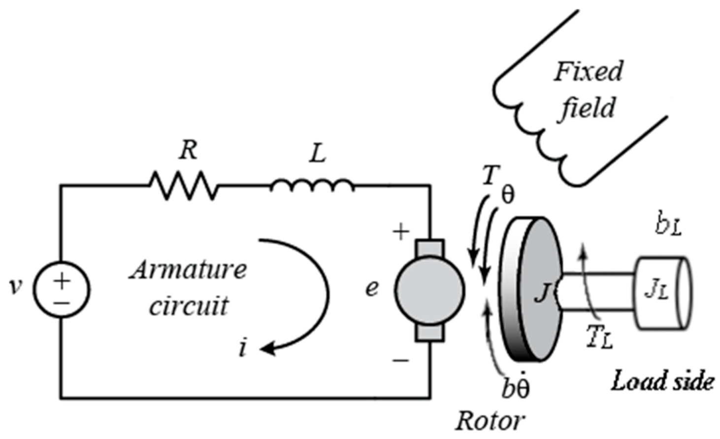
Figure 3.
Diagram of the digital twin model.
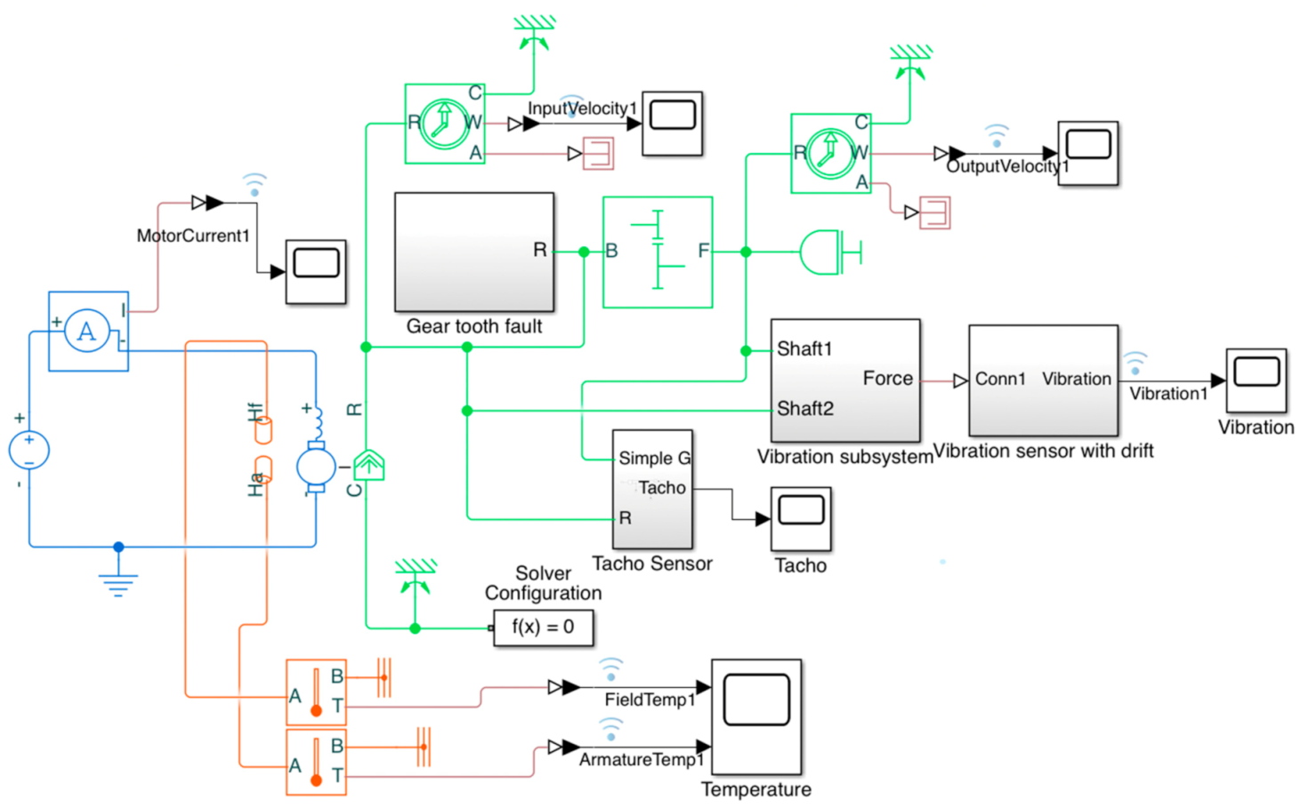
Figure 4.
A visualization for gearbox tooth faults [18].
Figure 4.
A visualization for gearbox tooth faults [18].

Figure 5.
Predictive maintenance workflow.

Figure 6.
Result of the power spectra analysis.

Figure 7.
Effect of the preprocessing step proposed above, on an example vibration signal: (a) Vibration data before the proposed preprocessing step; (b) Vibration data after the proposed preprocessing step.
Figure 7.
Effect of the preprocessing step proposed above, on an example vibration signal: (a) Vibration data before the proposed preprocessing step; (b) Vibration data after the proposed preprocessing step.

Figure 8.
Overall flowchart of the proposed workflow.
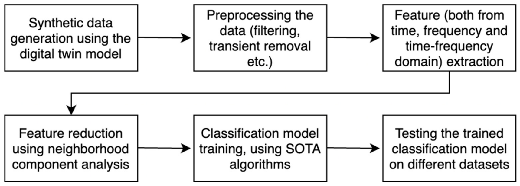
Figure 9.
Accuracy results for different algorithms for the CWRU dataset.
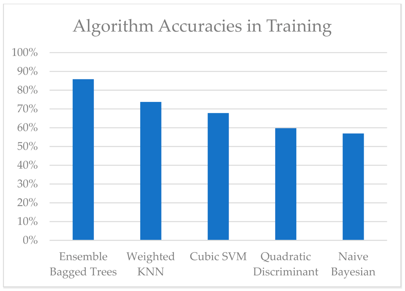
Figure 10.
Accuracy results for different algorithms for the synthetic data.

Figure 11.
Features vs. classes graphs for the synthetic data with ensemble bagged tree algorithm: (a) Feature vs. classes graphs for mean, median, variance, peak value, skewness and kurtosis; (b) Feature vs. classes graphs for RMS value, MAD, peak-to-peak value, approximate entropy, crest factor and high-frequency power; (c) Feature vs. classes graphs for range of cumulative sum, correlation dimension, Lyapunov exponent, peak frequency, envelope power and spectral kurtosis.

Publisher’s Note: MDPI stays neutral with regard to jurisdictional claims in published maps and institutional affiliations. |
© 2021 by the authors. Licensee MDPI, Basel, Switzerland. This article is an open access article distributed under the terms and conditions of the Creative Commons Attribution (CC BY) license (https://creativecommons.org/licenses/by/4.0/).
Share and Cite
MDPI and ACS Style
Selçuk, Ş.Y.; Ünal, P.; Albayrak, Ö.; Jomâa, M. A Workflow for Synthetic Data Generation and Predictive Maintenance for Vibration Data. Information 2021, 12, 386. https://0-doi-org.brum.beds.ac.uk/10.3390/info12100386
AMA Style
Selçuk ŞY, Ünal P, Albayrak Ö, Jomâa M. A Workflow for Synthetic Data Generation and Predictive Maintenance for Vibration Data. Information. 2021; 12(10):386. https://0-doi-org.brum.beds.ac.uk/10.3390/info12100386
Chicago/Turabian StyleSelçuk, Şahan Yoruç, Perin Ünal, Özlem Albayrak, and Moez Jomâa. 2021. "A Workflow for Synthetic Data Generation and Predictive Maintenance for Vibration Data" Information 12, no. 10: 386. https://0-doi-org.brum.beds.ac.uk/10.3390/info12100386
Note that from the first issue of 2016, this journal uses article numbers instead of page numbers. See further details here.