
Detecting and Mitigating Adversarial Examples in Regression Tasks: A Photovoltaic Power Generation Forecasting Case Study

 , , and
Abstract
:1. Introduction
- A novel scheme able to detect and mitigate adversarial attacks on DL regression models;
- A study of adversarial attacks on photovoltaic power generation forecasting;
- A comparison of Long-Short Term Memory (LSTM) and Temporal Convolutional Network (TCN) when under attack;
- An investigation regarding One-class Support Vector Machine (OCSVM) and Local Outlier Factor (LOF) as detectors of adversarial examples.
2. Background
2.1. Time Series
2.2. Adversarial Machine Learning
2.2.1. Attack Classification
- A white-box attack, which implies that the attacker has access to the entire set of components.
- A black-box attack, which implies that the attacker lacks substantial knowledge about the system components.
- A gray-box attack, which lies between the previous attacks. In this case, the attacker may have partial access to the training data, knowing the training algorithm or the feature space.
2.2.2. Adversarial Examples Generation
2.2.3. Defense Approaches
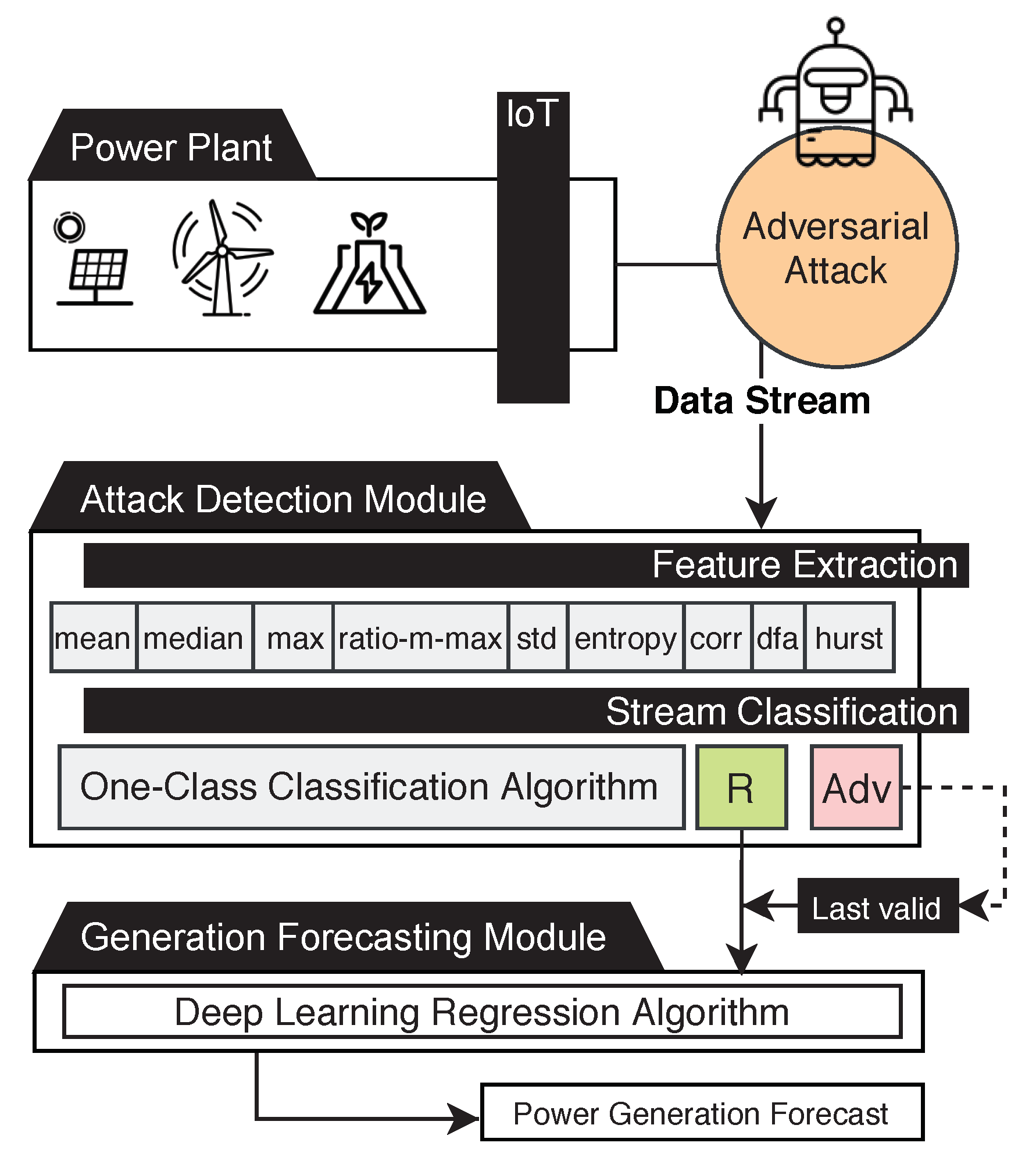
3. Proposed Approach
4. Materials and Methods
4.1. Dataset
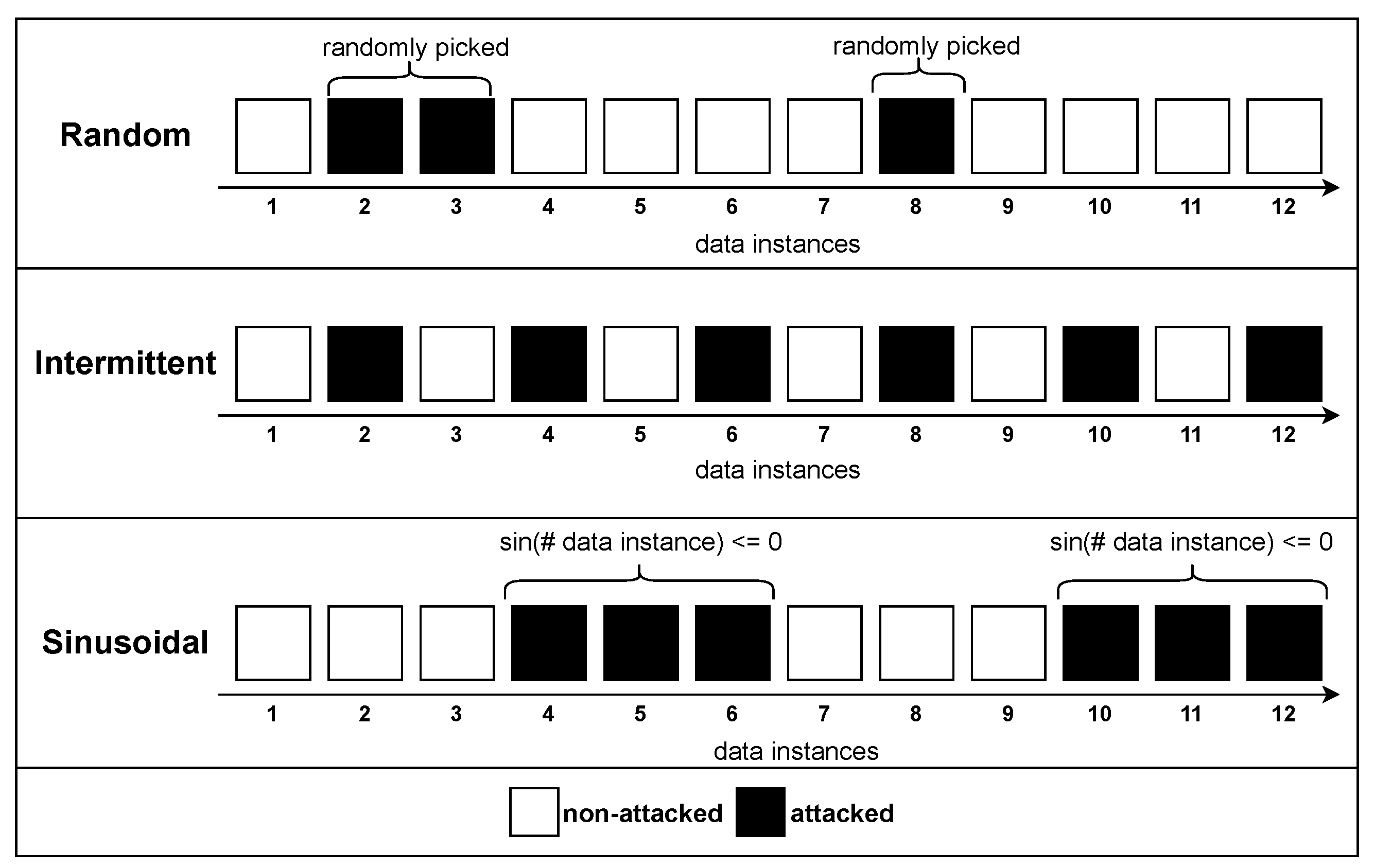
4.2. Threat Model
4.3. Attack Detection Module
4.4. Generation Forecasting Module
4.5. Evaluation Metrics
5. Results and Discussion
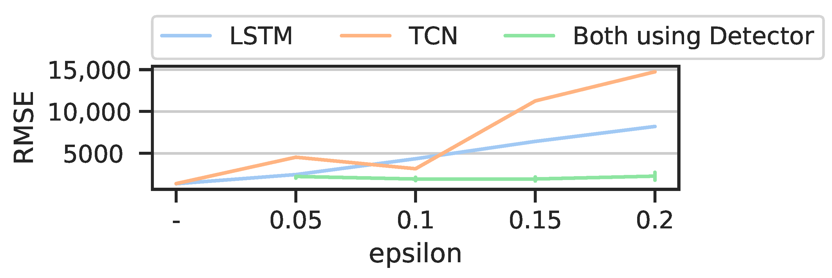
5.1. Adversarial Examples’ Mitigation
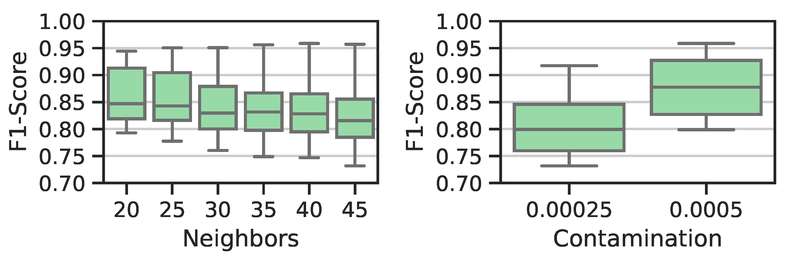
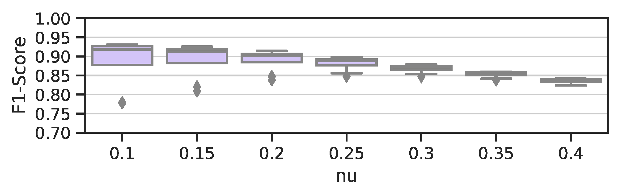
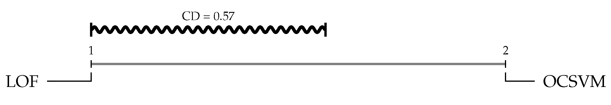
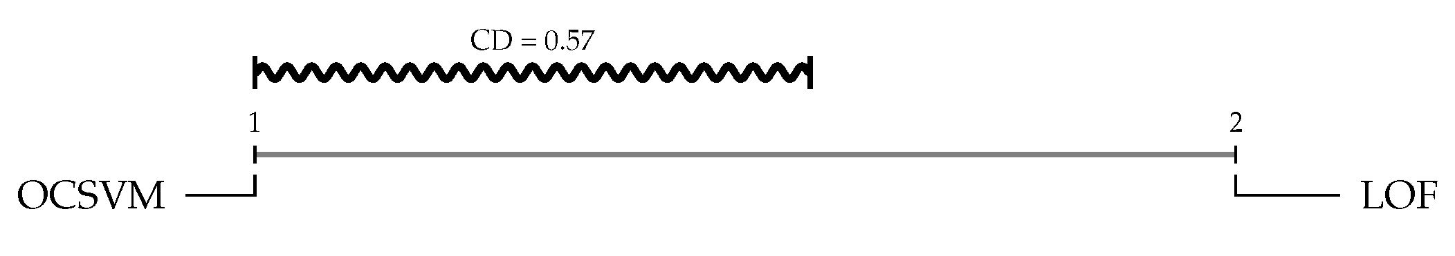
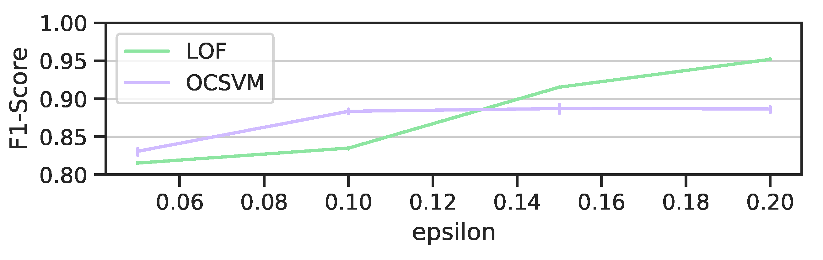
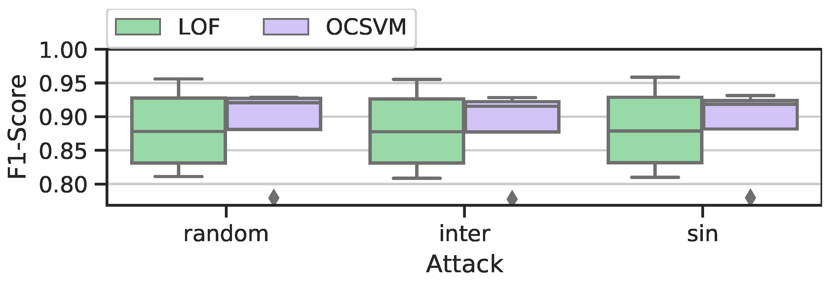
5.2. Attack Detection Module’s Efficacy in Detecting Adversarial Examples
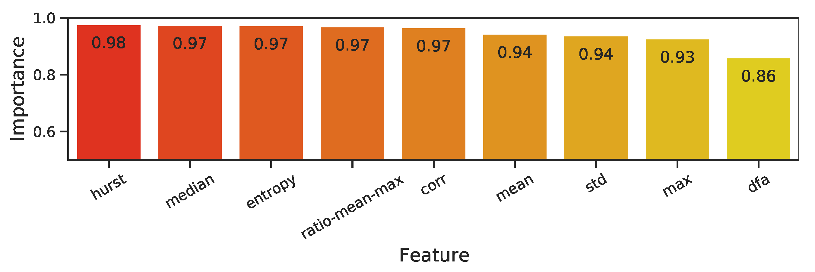
5.3. Feature Importance
5.4. Discussion
6. Conclusions
Author Contributions
Funding
Institutional Review Board Statement
Informed Consent Statement
Data Availability Statement
Conflicts of Interest
Abbreviations
| ARIMA | Autoregressive Integrated Moving Average |
| BIM | Basic Iterative Method |
| CD | Critical Difference |
| CNN | Convolutional Neural Network |
| DL | Deep Learning |
| DFA | Detrended Fluctuation Analysis |
| DTW | Dynamic Time Warping |
| FCN | Fully Convolutional Network |
| FGSM | Fast Gradient Sign Method |
| JSMA | Jacobian-based Saliency Map Attack |
| LOF | Local Outlier Factor |
| LR | Logistic Regression |
| LSTM | Long Short-term Memory Network |
| ML | Machine Learning |
| OCSVM | One Class Support Vector Machine |
| PV | Photovoltaic |
| ReLU | Rectified Linear Unit |
| RMSE | Root Mean Squared Error |
| RNN | Recurrent Neural Networks |
| SPEC | Spectral Feature Selection for Supervised and Unsupervised Learning |
| TCN | Temporal Convolutional Neural Network |
References
- Das, U.K.; Tey, K.S.; Seyedmahmoudian, M.; Mekhilef, S.; Idris, M.Y.I.; Van Deventer, W.; Horan, B.; Stojcevski, A. Forecasting of photovoltaic power generation and model optimization: A review. Renew. Sustain. Energy Rev. 2018, 81, 912–928. [Google Scholar] [CrossRef]
- López-Vargas, A.; Fuentes, M.; Vivar, M. IoT Application for Real-Time Monitoring of Solar Home Systems Based on Arduino™ With 3G Connectivity. IEEE Sens. J. 2019, 19, 679–691. [Google Scholar] [CrossRef]
- Antonanzas, J.; Osorio, N.; Escobar, R.; Urraca, R.; Martinez-de Pison, F.J.; Antonanzas-Torres, F. Review of photovoltaic power forecasting. Sol. Energy 2016, 136, 78–111. [Google Scholar] [CrossRef]
- Wang, K.; Qi, X.; Liu, H. A comparison of day-ahead photovoltaic power forecasting models based on deep learning neural network. Appl. Energy 2019, 251, 113315. [Google Scholar] [CrossRef]
- Yen, C.F.; Hsieh, H.Y.; Su, K.W.; Leu, J.S. Predicting Solar Performance Ratio Based on Encoder-Decoder Neural Network Model. In Proceedings of the 2019 11th International Congress on Ultra Modern Telecommunications and Control Systems and Workshops (ICUMT), Dublin, Ireland, 28–30 October 2019; pp. 1–4. [Google Scholar]
- Ibrahim, M.S.; Dong, W.; Yang, Q. Machine learning driven smart electric power systems: Current trends and new perspectives. Appl. Energy 2020, 272, 115237. [Google Scholar] [CrossRef]
- Fawaz, H.I.; Forestier, G.; Weber, J.; Idoumghar, L.; Muller, P.A. Adversarial attacks on deep neural networks for time series classification. In Proceedings of the 2019 International Joint Conference on Neural Networks (IJCNN), Budapest, Hungary, 14–19 July 2019; pp. 1–8. [Google Scholar]
- Hua, B.; Zhang, K.; Wei, H.; Zhang, J.; Xie, L. A Multilevel Fire Detection Platform Based on Multi-Source Heterogeneous Information Fusion. In Proceedings of the 2020 International Conference on Pattern Recognition and Intelligent Systems, Athens, Greece, 30 July–2 August 2020; pp. 1–5. [Google Scholar]
- Kumar, R.S.S.; Nyström, M.; Lambert, J.; Marshall, A.; Goertzel, M.; Comissoneru, A.; Swann, M.; Xia, S. Adversarial machine learning-industry perspectives. In Proceedings of the 2020 IEEE Security and Privacy Workshops (SPW), San Francisco, CA, USA, 21–21 May 2020; pp. 69–75. [Google Scholar]
- Niazazari, I.; Livani, H. Attack on Grid Event Cause Analysis: An Adversarial Machine Learning Approach. In Proceedings of the 2020 IEEE Power & Energy Society Innovative Smart Grid Technologies Conference (ISGT), Washington, DC, USA, 17–20 February 2020; pp. 1–5. [Google Scholar]
- Karim, F.; Majumdar, S.; Darabi, H. Adversarial attacks on time series. IEEE Trans. Pattern Anal. Mach. Intell. 2020, 43, 3309–3320. [Google Scholar] [CrossRef] [Green Version]
- Abdu-Aguye, M.G.; Gomaa, W.; Makihara, Y.; Yagi, Y. Detecting Adversarial Attacks In Time-Series Data. In Proceedings of the ICASSP 2020-2020 IEEE International Conference on Acoustics, Speech and Signal Processing (ICASSP), Barcelona, Spain, 4–8 May 2020; pp. 3092–3096. [Google Scholar]
- Santana, E.J.; Silva, R.P.; Zarpelão, B.B.; Barbon Junior, S. Photovoltaic Generation Forecast: Model Training and Adversarial Attack Aspects. In Proceedings of the Brazilian Conference on Intelligent Systems, Rio Grande, Brazil, 20–23 October 2020; pp. 634–649. [Google Scholar]
- Parzen, E. An approach to time series analysis. Ann. Math. Stat. 1961, 32, 951–989. [Google Scholar] [CrossRef]
- Tabassi, E.; Burns, K.J.; Hadjimichael, M.; Molina-Markham, A.D.; Sexton, J.T. A Taxonomy and Terminology of Adversarial Machine Learning. NIST IR 2019, 1–29. [Google Scholar] [CrossRef]
- Biggio, B.; Roli, F. Wild patterns: Ten years after the rise of adversarial machine learning. Pattern Recognit. 2018, 84, 317–331. [Google Scholar] [CrossRef] [Green Version]
- Papernot, N.; McDaniel, P.; Goodfellow, I. Transferability in machine learning: From phenomena to black-box attacks using adversarial samples. arXiv 2016, arXiv:1605.07277. [Google Scholar]
- Yuan, X.; He, P.; Zhu, Q.; Li, X. Adversarial examples: Attacks and defenses for deep learning. IEEE Trans. Neural Netw. Learn. Syst. 2019, 30, 2805–2824. [Google Scholar] [CrossRef] [PubMed] [Green Version]
- Goodfellow, I.J.; Shlens, J.; Szegedy, C. Explaining and harnessing adversarial examples. arXiv 2014, arXiv:1412.6572. [Google Scholar]
- Rozsa, A.; Rudd, E.M.; Boult, T.E. Adversarial diversity and hard positive generation. In Proceedings of the IEEE Conference on Computer Vision and Pattern Recognition Workshops, Las Vegas, NV, USA, 27–30 June 2016; pp. 25–32. [Google Scholar]
- Dong, Y.; Liao, F.; Pang, T.; Su, H.; Zhu, J.; Hu, X.; Li, J. Boosting adversarial attacks with momentum. In Proceedings of the IEEE Conference on Computer Vision and Pattern Recognition, Salt Lake City, UT, USA, 18–23 June 2018; pp. 9185–9193. [Google Scholar]
- Papernot, N.; McDaniel, P.; Wu, X.; Jha, S.; Swami, A. Distillation as a defense to adversarial perturbations against deep neural networks. In Proceedings of the 2016 IEEE Symposium on Security and Privacy (SP), San Jose, CA, USA, 22–26 May 2016; pp. 582–597. [Google Scholar]
- Tian, J.; Li, T.; Shang, F.; Cao, K.; Li, J.; Ozay, M. Adaptive Normalized Attacks for Learning Adversarial Attacks and Defenses in Power Systems. In Proceedings of the 2019 IEEE International Conference on Communications, Control, and Computing Technologies for Smart Grids (SmartGridComm), Beijing, China, 21–23 October 2019; pp. 1–6. [Google Scholar]
- Liu, X.; Cheng, M.; Zhang, H.; Hsieh, C.J. Towards robust neural networks via random self-ensemble. In Proceedings of the European Conference on Computer Vision (ECCV), Munich, Germany, 8–14 September 2018; pp. 369–385. [Google Scholar]
- Meng, D.; Chen, H. Magnet: A two-pronged defense against adversarial examples. In Proceedings of the 2017 ACM SIGSAC Conference on Computer and Communications Security, Dallas, TX, USA, 15 September 2017; pp. 135–147. [Google Scholar]
- Lu, J.; Issaranon, T.; Forsyth, D. Safetynet: Detecting and rejecting adversarial examples robustly. In Proceedings of the IEEE International Conference on Computer Vision, Venice, Italy, 22–29 October 2017; pp. 446–454. [Google Scholar]
- Zarpelão, B.B.; Barbon, S.; Acarali, D.; Rajarajan, M. How Machine Learning Can Support Cyberattack Detection in Smart Grids. In Artificial Intelligence Techniques for a Scalable Energy Transition; Springer: Berlin/Heidelberg, Germany, 2020; pp. 225–258. [Google Scholar]
- Martins, N.; Cruz, J.M.; Cruz, T.; Abreu, P.H. Adversarial machine learning applied to intrusion and malware scenarios: A systematic review. IEEE Access 2020, 8, 35403–35419. [Google Scholar] [CrossRef]
- Li, J.; Yang, Y.; Sun, J.S.; Tomsovic, K.; Qi, H. Conaml: Constrained adversarial machine learning for cyber-physical systems. In Proceedings of the 2021 ACM Asia Conference on Computer and Communications Security, Hong Kong, China, 7–11 June 2021; pp. 52–66. [Google Scholar]
- Duy, P.T.; Khoa, N.H.; Nguyen, A.G.T.; Pham, V.H. DIGFuPAS: Deceive IDS with GAN and Function-Preserving on Adversarial Samples in SDN-enabled networks. Comput. Secur. 2021, 109, 102367. [Google Scholar] [CrossRef]
- Anthi, E.; Williams, L.; Javed, A.; Burnap, P. Hardening machine learning denial of service (DoS) defenses against adversarial attacks in IoT smart home networks. Comput. Secur. 2021, 108, 102352. [Google Scholar] [CrossRef]
- Chen, Y.; Tan, Y.; Deka, D. Is machine learning in power systems vulnerable? In Proceedings of the 2018 IEEE International Conference on Communications, Control, and Computing Technologies for Smart Grids (SmartGridComm), Aalborg, Denmark, 29–31 October 2018; pp. 1–6. [Google Scholar]
- Bulusu, S.; Kailkhura, B.; Li, B.; Varshney, P.; Song, D. Anomalous Instance Detection in Deep Learning: A Survey; Technical Report; Lawrence Livermore National Lab.(LLNL): Livermore, CA, USA, 2020. [Google Scholar]
- Kontouras, E.; Tzes, A.; Dritsas, L. Hybrid Detection of Intermittent Cyber-Attacks in Networked Power Systems. Energies 2019, 12, 4625. [Google Scholar] [CrossRef] [Green Version]
- Schölzel, C. Nonlinear Measures for Dynamical Systems. 2019. Available online: https://zenodo.org/record/3814723#.YUzRj7hKjIU (accessed on 1 September 2021).
- Cortes, C.; Vapnik, V. Support-vector networks. Mach. Learn. 1995, 20, 273–297. [Google Scholar] [CrossRef]
- Breunig, M.M.; Kriegel, H.P.; Ng, R.T.; Sander, J. LOF: Identifying density-based local outliers. In Proceedings of the 2000 ACM SIGMOD International Conference on Management of Data, Dallas, TX, USA, 16–18 May 2000; pp. 93–104. [Google Scholar]
- Peng, W.; Liu, R.; Wang, R.; Cheng, T.; Wu, Z.; Cai, L.; Zhou, W. EnsembleFool: A method to generate adversarial examples based on model fusion strategy. Comput. Secur. 2021, 107, 102317. [Google Scholar] [CrossRef]
- Appiah, B.; Qin, Z.; Abra, A.M.; Kanpogninge, A.J.A. Decision tree pairwise metric learning against adversarial attacks. Comput. Secur. 2021, 106, 102268. [Google Scholar] [CrossRef]
- Cerqueira, V.; Torgo, L.; Soares, C. Machine Learning vs Statistical Methods for Time Series Forecasting: Size Matters. arXiv 2019, arXiv:1909.13316. [Google Scholar]
- Hochreiter, S.; Schmidhuber, J. Long short-term memory. Neural Comput. 1997, 9, 1735–1780. [Google Scholar] [CrossRef]
- Kim, D.; Kwon, D.; Park, L.; Kim, J.; Cho, S. Multiscale LSTM-Based Deep Learning for Very-Short-Term Photovoltaic Power Generation Forecasting in Smart City Energy Management. IEEE Syst. J. 2020, 15, 346–354. [Google Scholar] [CrossRef]
- Ahmed, R.; Sreeram, V.; Mishra, Y.; Arif, M. A review and evaluation of the state-of-the-art in PV solar power forecasting: Techniques and optimization. Renew. Sustain. Energy Rev. 2020, 124, 109792. [Google Scholar] [CrossRef]
- Zhao, Z.; Liu, H. Spectral feature selection for supervised and unsupervised learning. In Proceedings of the 24th International Conference on Machine Learning, Corvalis, OR, USA, 20–24 June 2007; pp. 1151–1157. [Google Scholar]


| Reference | Dataset | Model | Output | Attack | Transferability | Defence |
|---|---|---|---|---|---|---|
| Chen et al. (2018) | Simulated data on power quality and building load | NN and RNN | C and R | FGSM | Yes | - |
| Favaz et al. (2019) | Several univariate time series | ResNet | C | FGSM and BIM | No | - |
| Niazazari and Livani (2020) | Simulated data of grid events | CNN | C | FGSM and JSMA | No | Adversarial training |
| Karim et al. (2020) | Several time series datasets | 1-NN DTW and FCN | C | FGSM and ATN | No | Adversarial training |
| Abdu-Aguye et al. (2020) | Several univariate time series | ResNet | C | FGSM and BIM | No | OC-SVM |
| Parameters | Experimented Hyper-Parameters | |
|---|---|---|
| LSTM | Number of stacked layers | 1, 2, 3 |
| Units | 32, 64, 128 | |
| TCN | Number of filters | 32, 64 |
| Kernel | 2, 3 | |
| Dilations | [1, 4, 12, 48], [1, 2, 4, 8, 12, 24, 48], [1, 4, 16, 32], [1, 2, 4, 8, 16, 32], [1, 3, 6, 12, 24], [1, 2, 6, 12, 24], [1, 2, 4, 8, 16], [1, 4, 16], [1, 2, 4, 8], [1, 4, 8] | |
| Blocks | 1, 2 |
| Detector | Forecast RMSE * (% **) | ||
|---|---|---|---|
| LSTM | TCN | ||
| - | - | 1370.35 | 1388.24 |
| 0.05 | - | 2466.18 (79.97%) | 4538.75 (226.94%) |
| 0.10 | - | 4356.53 (217.91%) | 3160.94 (127.69%) |
| 0.15 | - | 6427.32 (369.03%) | 11,261.55 (711.21%) |
| 0.20 | - | 8213.34 (499.36%) | 14,746.09 (962.21%) |
| 0.05 | OCSVM | 2433.76 (77.60%) | 2087.62 (50.38%) |
| 0.10 | OCSVM | 2143.56 (56.42%) | 1764.01(27.07%) |
| 0.15 | OCSVM | 2198.36 (60.42%) | 1729.19 (24.56%) |
| 0.20 | OCSVM | 2921.47 (113.19%) | 2358.44(69.89%) |
| 0.05 | LOF | 2427.25 (77.13%) | 2008.58 (44.68%) |
| 0.10 | LOF | 2116.04 (54.42%) | 1719.30 (23.85%) |
| 0.15 | LOF | 2161.84 (57.76%) | 1661.70 (19.70%) |
| 0.20 | LOF | 2145.56 (56.57%) | 1686.87 (21.51%) |
Publisher’s Note: MDPI stays neutral with regard to jurisdictional claims in published maps and institutional affiliations. |
© 2021 by the authors. Licensee MDPI, Basel, Switzerland. This article is an open access article distributed under the terms and conditions of the Creative Commons Attribution (CC BY) license (https://creativecommons.org/licenses/by/4.0/).
Share and Cite
Santana, E.J.; Silva, R.P.; Zarpelão, B.B.; Barbon Junior, S. Detecting and Mitigating Adversarial Examples in Regression Tasks: A Photovoltaic Power Generation Forecasting Case Study. Information 2021, 12, 394. https://0-doi-org.brum.beds.ac.uk/10.3390/info12100394
Santana EJ, Silva RP, Zarpelão BB, Barbon Junior S. Detecting and Mitigating Adversarial Examples in Regression Tasks: A Photovoltaic Power Generation Forecasting Case Study. Information. 2021; 12(10):394. https://0-doi-org.brum.beds.ac.uk/10.3390/info12100394
Chicago/Turabian StyleSantana, Everton Jose, Ricardo Petri Silva, Bruno Bogaz Zarpelão, and Sylvio Barbon Junior. 2021. "Detecting and Mitigating Adversarial Examples in Regression Tasks: A Photovoltaic Power Generation Forecasting Case Study" Information 12, no. 10: 394. https://0-doi-org.brum.beds.ac.uk/10.3390/info12100394