
Pear Defect Detection Method Based on ResNet and DCGAN


College of Information and Electrical Engineering, China Agricultural University, Beijing 100083, China
*
Author to whom correspondence should be addressed.
†
These authors contributed equally to this work.
Information 2021, 12(10), 397; https://0-doi-org.brum.beds.ac.uk/10.3390/info12100397
Submission received: 12 August 2021
/
Revised: 8 September 2021
/
Accepted: 13 September 2021
/
Published: 28 September 2021
(This article belongs to the Special Issue Artificial Intelligence and Neural Networks at the Intersection of Society, Business, and Science)
Abstract
:To address the current situation, in which pear defect detection is still based on a workforce with low efficiency, we propose the use of the CNN model to detect pear defects. Since it is challenging to obtain defect images in the implementation process, a deep convolutional adversarial generation network was used to augment the defect images. As the experimental results indicated, the detection accuracy of the proposed method on the 3000 validation set was as high as 97.35%. Variant mainstream CNNs were compared to evaluate the model’s performance thoroughly, and the top performer was selected to conduct further comparative experiments with traditional machine learning methods, such as support vector machine algorithm, random forest algorithm, and k-nearest neighbor clustering algorithm. Moreover, the other two varieties of pears that have not been trained were chosen to validate the robustness and generalization capability of the model. The validation results illustrated that the proposed method is more accurate than the commonly used algorithms for pear defect detection. It is robust enough to be generalized well to other datasets. In order to allow the method proposed in this paper to be applied in agriculture, an intelligent pear defect detection system was built based on an iOS device.
1. Introduction
As the prominent component of the modern agriculture industry, the pear industry is quite sensitive to the products’ quality and overall profits [1]. One of the crucial evaluation criteria of pear grade is the defect of pears, for example, blackspot [2], one of the relatively pervasive pear defects. Once the defect occurs and corresponding treatments are not taken in time, a series of fruits cracking and falling will follow irreversibly, resulting in significant economic losses. At present, the detection of pear defects still relies on a labor workforce, with long working hours, high cost, and low efficiency. With the prosperity of computer vision technology, plenty of artificial neural network structures have been proposed and applied in various fields, with significant advantages. As regards pear blackspot, the traditional detection method is time-consuming and inefficient. With the flourishing of convolutional neural networks in computer vision, various network structures based on them have been applied to pear defect detection and achieved terrific results.
A convolutional neural network can effectively overcome the demerits mentioned above. Lecun put forward LeNet in 1999 [3], while Alexei won the ImageNet image recognition race champion and slashed the top-5 error in 2012 [4]. During this period, further research led to the boom of convolutional neural networks. The convolutional neural network was rapidly popularized in wide application scenarios of computer vision and made a breakthrough in agricultural production. For instance, the LeNet-5 network model was improved by Lichao Zhang et al. [5] and used for crop variety identification. The detection accuracy was as high as 93.7%, which was considerably increased in this domain. Additionally, crop lesions were detected based on DBN (Deep Belief Nets) structure by Zhaoyong Zhou et al. [6], and this practice has proved it works better than the traditional algorithm.
In recent years, with the continuous rise of Kaggle and ImageNet visual data mining and computer network events, several brilliant convolutional neural network structures with superior properties have emerged, such as the VGG series [7], ResNet series [8], GoogLeNet series [9], and DenseNet series [10]. All the network structures above have obtained the ImageNet Challenge’s championship and proven their outstanding robustness and generalization capability in many kinds of product identification and positioning problems. Hitherto, the pear defect detection still mainly depends on the traditional algorithm, such as the support vector machine (SVM) algorithm [11]. Yet, the convolutional neural network use in agriculture remains rarely investigated [12,13,14].
In this study, we adopted the accuracy parameter to conduct experiments, and ResNet50 was compared with mainstream CNNs, including the champion network of the ImageNet Challenge and traditional algorithms. Experiments indicated that after data enhancement and augmentation and using warm-up and other training techniques, ResNet50 could reach an accuracy of 97.35%.
Since a convolutional neural network requires a lot of data for training, and image data of defective pears are usually tricky to obtain in reality, the deep convolutional adversarial generation network was used to train fewer real defective images. It automatically generated defective images to provide training materials for CNNs, which could balance the unbalanced positive and negative sample ratio and achieve good results.
2. Materials and Methods
2.1. Experimental Materials and System Configuration
In this paper, Korla pear [15] in Xinjiang was selected as the empirical material. The image acquisition equipment was Apple’s intelligent mobile terminal, and the lighting equipment was BenQ Wit. The pear was placed on the rotating tripod head in the vertical direction of the calyx and horizontal direction to the ground. A total of 2000 images were taken, including 1500 positive samples and 500 negative samples, as shown in Table 1.
The experiment was completed in Ubuntu operating system. The computer is configured as Intel i9, the memory is 16 GB, and the GPU is GeForce RTX 3080. The experimental conclusions and code in this paper are based on Python 3.9.
2.2. Data Pre-Processing
2.2.1. Data Augmentation
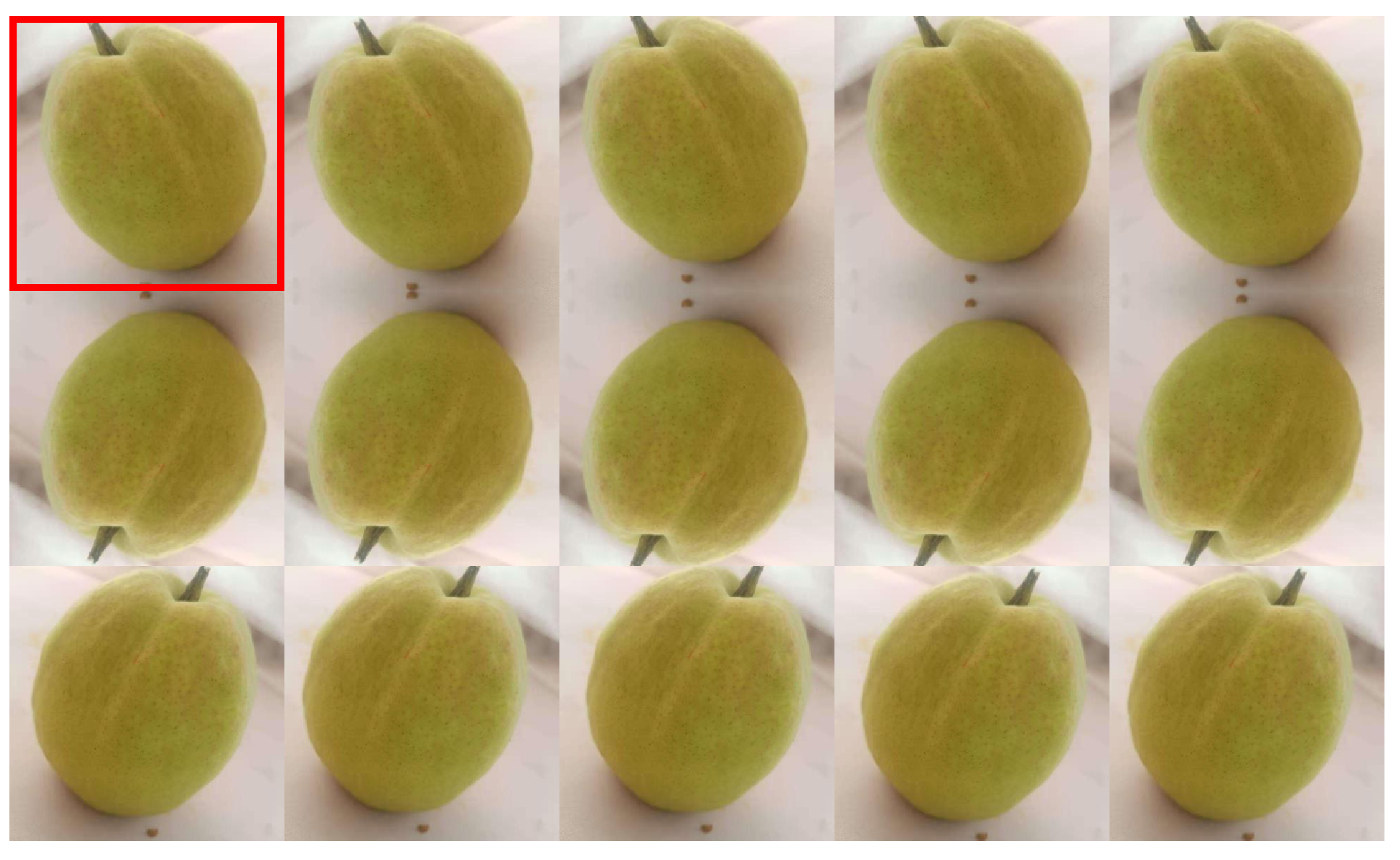
Data augmentation is a standard pre-processing tool in computer vision, mainly to solve the performance degradation problem caused by inadequate training or overfitting of the network due to insufficient data. Traditional data augmentation methods include image translation, image rotation, image flipping, image horizontal, and vertical flipping, image cropping, and repositioning. This paper referred to the method proposed by Alex et al. First of all, every image was cropped by cutting out five parts, which were then flipped horizontally and vertically. As shown in Figure 1, each original image will eventually generate fifteen augmented images.
2.2.2. Image Graying
The color value of each pixel on a grayscale image is called grayscale [16]. Image graying can be used as a pre-processing step in image processing to prepare for later higher-level operations such as image segmentation, image recognition, and image analysis.
The image we collected is in the RGB color mode, and the three RGB components are disposed of separately when processed. Nevertheless, in the defect detection problem faced here, RGB does not reflect the morphological features of the picture but only blends colors from the principle of optics.
Since the visual features of the defect can still be retained after image graying, converting it into grayscale images can cut down the number of parameters of the model and accelerate the training and inference session. As shown in Figure 2, the colorful RGB three-channel images are hence grayed out firstly.
2.2.3. Dilation and Erosion
Erosion and dilation [17] belong to the morphological scope, where the logical expression of the dilation operation is shown as follows:
The logical expression of the erosion operation is formulated as:
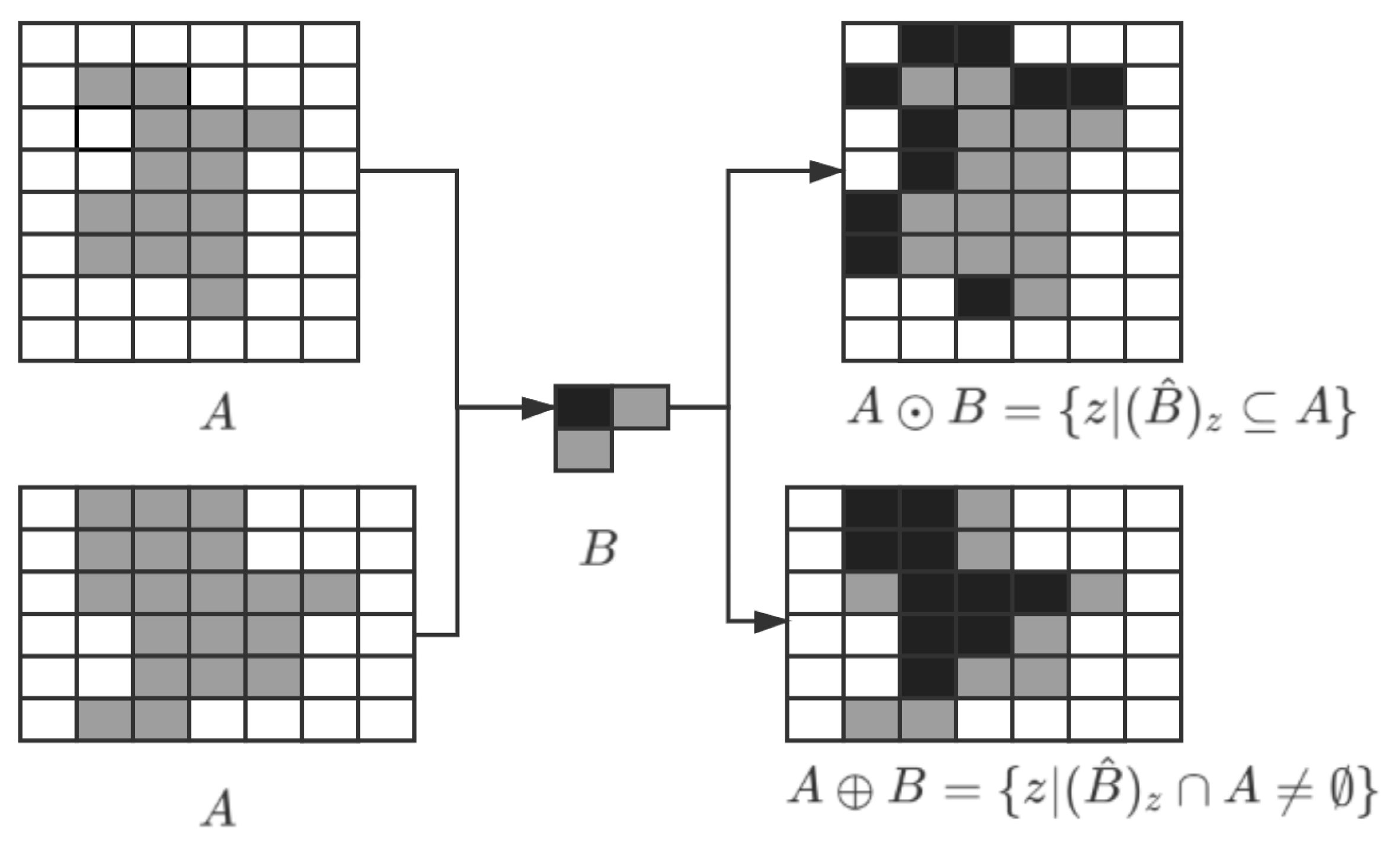
In the field of graphics, dilation and corrosion techniques are known as morphological manipulation of binary images. Dilation expands and magnifies bright areas in a photo by adding pixels to the boundaries of objects in the picture. Erosion does the opposite, removing pixels along the borders of objects in the image and reducing their size. Usually, these two operations are performed sequentially to enhance essential features of objects in the picture. In Formulas (1) and (2), A represents the original image, and B represents the operator. The process of applying it to the binary graph is shown in Figure 3. B corresponds to a matrix core moving over the image, such as a filter, turning the pixel white if any surrounding pixel is white in the window.
An opening operation [18] can be realized through erosion and dilation, which can eliminate small objects and separate them at a satisfactory level and smooth the boundaries of large objects without significantly changing their areas. By applying the opening operation to the grayscale image, the typical fine spots on the pear surface can be lessened to avoid interfering with the model’s defect detection, as shown in Figure 4.
2.3. Data Augmentation Based on DCGAN
In our datasets, the extreme shortage of defective images, which accounted for only a quarter of the total datasets, and the imbalance of positive and negative samples, make CNN training difficult. For instance, the loss of the positive sample was higher than that of the negative samples, which led to an inability to acquire features of the negative samples; therefore, synthetic data generation is a crucial step before model training. In this paper, the Gaussian-based sampling method [19] was adopted to generate lesion images based on available conventional data. The two parameters required are the mean and standard deviation. The probability density distribution of Gaussian distribution is expressed as:
where x is the eigenvector. By varying the mean and standard data variance, the desired eigenvectors of defect images can be generated by sampling from the modified Gaussian distribution.
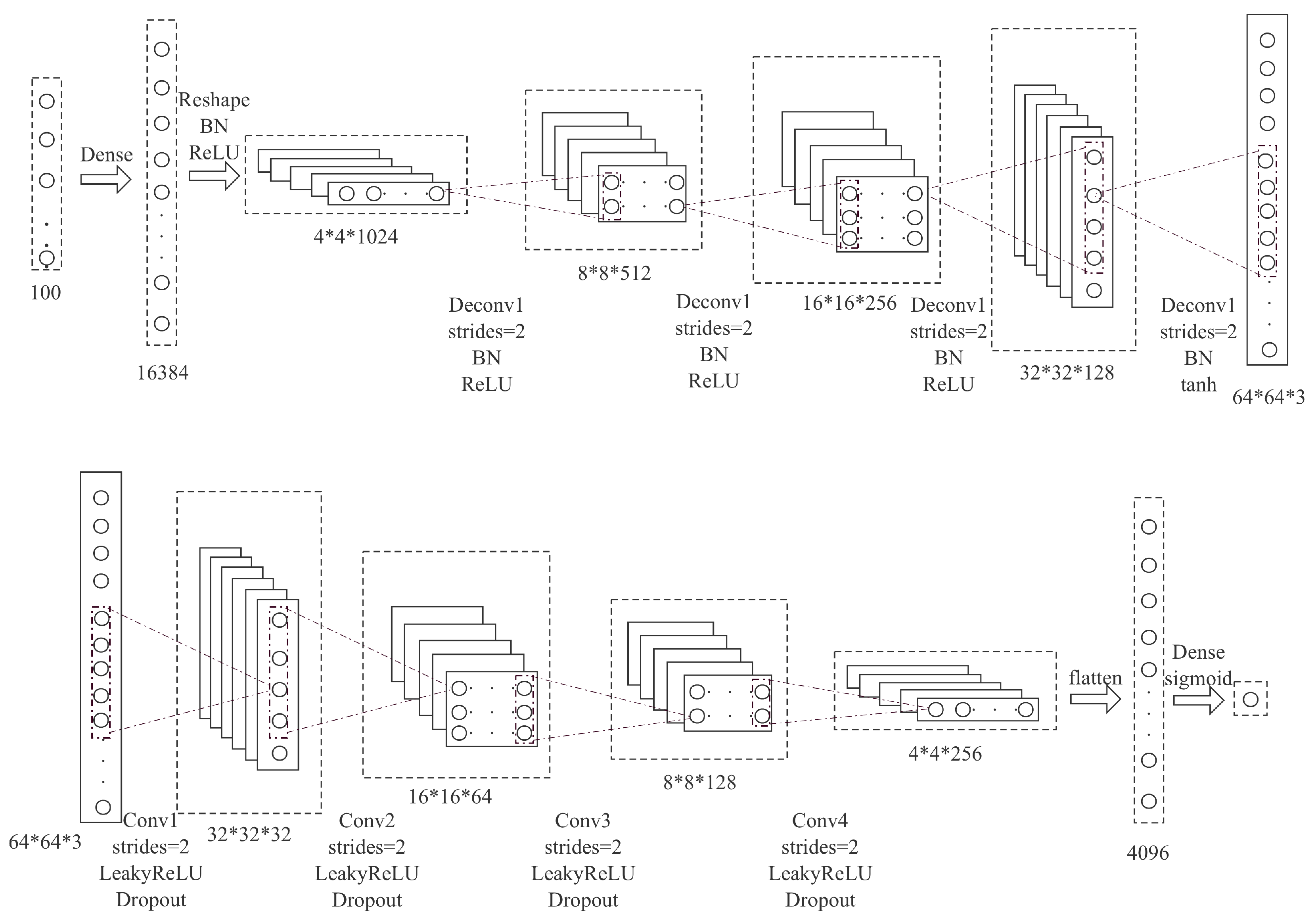
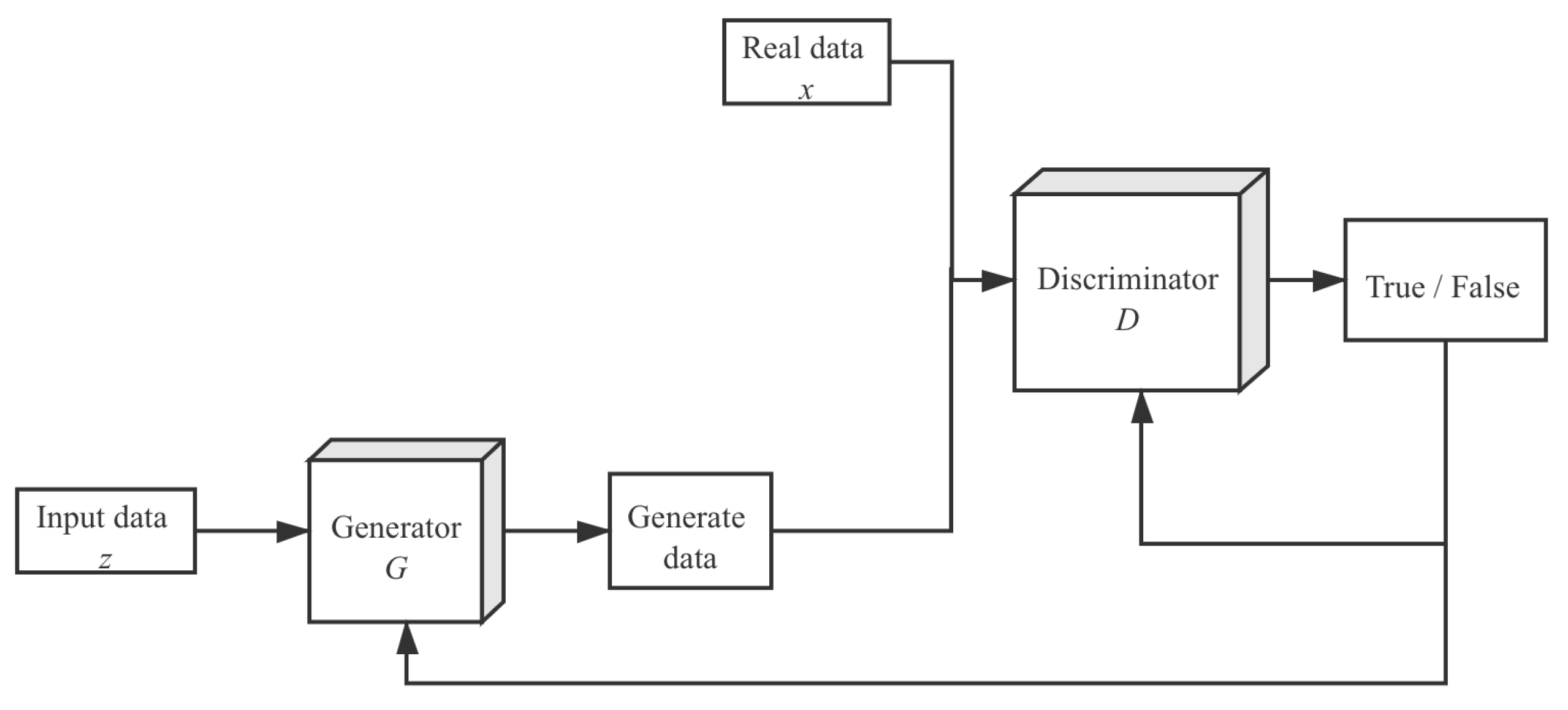
Given the available eigenvectors corresponding to the normal and defective ones, a synthetic data generator based on DCGAN [20] was conceived. The generator was used to produce more available eigenvectors corresponding to lesion images to enrich the training process. In the DCGAN, there were two participants: the generator G; and the discriminator D. Let denote the distribution of eigenvectors extracted from them. The goal of the generator model G was to generate probability distribution on the eigenvector data x. And this probability distribution was the estimated value of . Usually, the generator and discriminator are represented by two deep neural networks. The optimization objective of the DCGAN model can be mathematically represented as:
In Formula (4), x is the prior value of the input noise variable. During the training process, two deep neural network models were trained. The generative model G [21] and the discriminative model D [21] were pitted against each other by DCGAN. In other words, these two models will optimize their objective functions by playing games; however, to avoid finding the exact Nash balance that is challenging in the real world, the accuracy of the data generated in discriminator D was used as a stopping requirement. This means when the misclassified probability of the data generated from G is higher than a preset threshold, the training will stop. The training process is shown in Figure 5 and Figure 6.
2.4. ResNet Model Building
According to five models put forward in ResNet’s paper [8], the model structure was reformed in this paper. The input of the original model was RGB color three-channel images, while in this paper, the processed image was the grayscale image with one single channel. It is the 1000-classification task that the model mentioned in the original article aimed to achieve. In contrast, the problem processed in this paper was a binary classification problem, discriminating between defective pears and regular ones. Consequently, the in_planes parameter in the first convolution module of ResNet will be set to 1 (corresponding to the single-channel grayscale image); the num_classes parameter in the last fully connected layer will be set to 2, corresponding to the binary classification problems here.
Widely used in industry, ResNet is an ensemble of residual neural networks, including ResNet18, ResNet34, ResNet50, ResNet101, and ResNet152, where the numbers after the name represent parameter layers in need of training. In particular, the network layers of ResNet1202 are too deep to facilitate the training of small datasets, so it is inapplicable in most actual scenes, and the inspection of pears is no exception; therefore, the above five most frequently used models were taken as reference, whose parameters will be trained on the ImageNet datasets before being transferred for subsequent training and comparative experiments.
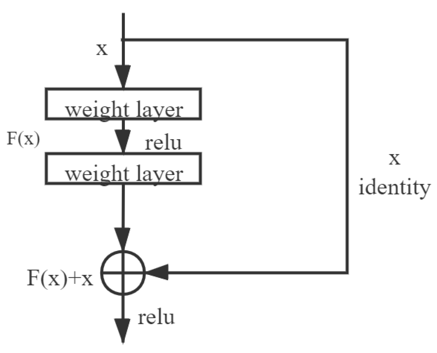
From a network structure introduced by ResNet, as shown in Figure 7, it can be seen that the residual structure guarantees that under no circumstances does the deep network work no worse than its corresponding shallower network. Before the structure was constructed, the dilemma haunted convolutional neural networks with the deepening of the network layer. The network performance declined once the depth reached a certain degree. The residual structure can effectively solve this problem.
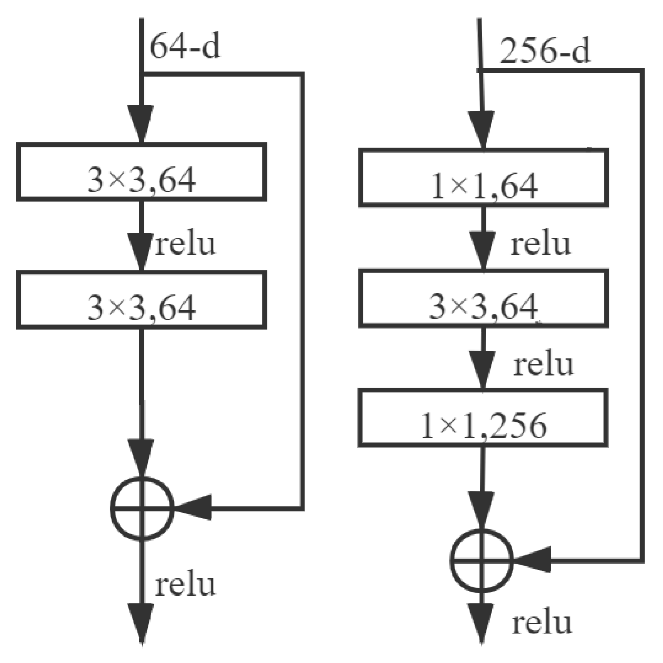
ResNet structure consists of 4 layers, and each layer contains multiple blocks divided into BasicBlock and Bottleneck. The BasicBlock has two convolution layers, two batch normalization layers, and two activation function layers. Bottleneck contains three convolution layers, three batch normalization layers, and three activation function layers. In the BasicBlock convolution layer, the convolution kernel size is 3 * 3. In the first and third Bottleneck convolution layers, the convolution kernel size is 1 * 1 for reducing and recovering the number of channels. In the middle convolution layer, i.e., the second layer, the convolution kernel size is 3 * 3.
BasicBlock and Bottleneck are two types of block in the ResNet where direct connections are neither between convolution layers nor blocks but between layers comprising blocks. The architecture is shown in Figure 8.
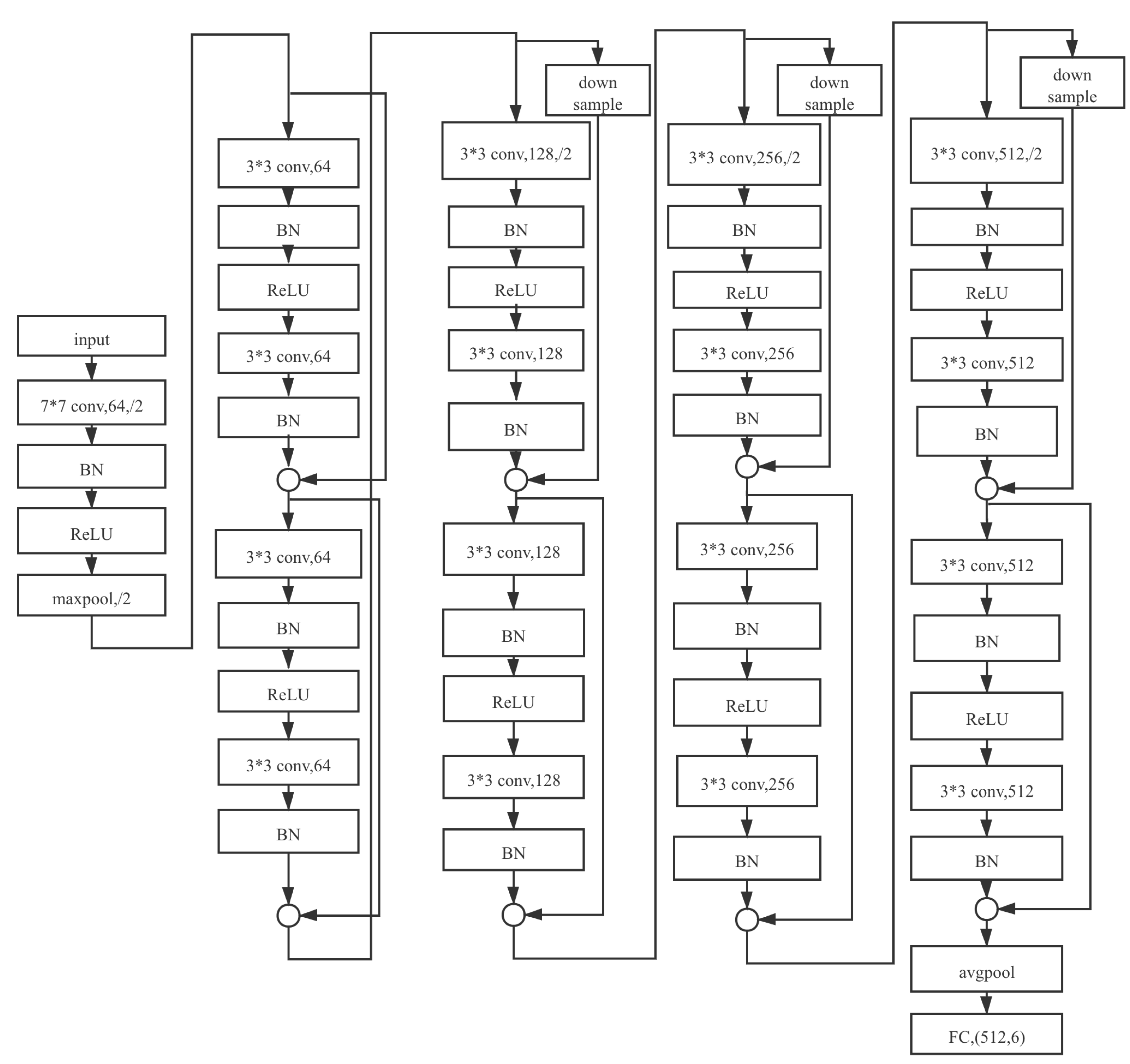
In the ResNet series, the types and counts of blocks in each layer vary from one network to another. ResNet18, whose architectures are shown in Figure 9 and ResNet34, are built with BasicBlock. While ResNet50, ResNet101, and ResNet152 are composed of Bottleneck. The block structures of them are shown in Table 2.
2.5. Model Training
2.5.1. Transfer Learning
Transfer learning is a machine learning method that can effectively use existing feature extraction and label classification networks to solve similar problems in different application scenarios. In addition to diminishing data dependency, transfer learning [22] can also raise the training efficiency of the network structure while speeding up the training.
After pre-training, the parameters of the convolution layer acting as feature extractor in the network structure have reached the optimal value, which were fixed during the first 50 iterations. That is, they did not execute the error back-propagation algorithm. The original classifier is designed for solving 1000-classification problems, whereas this paper tries to address the binary classification problem. Consequently, only parameters of the fully connected layer classifiers were adjusted through the first 50 iterations. In this way, the sheer quantity of model parameters that demanded to be trained was dramatically reduced. Hence, training times increased. All parameters in the network were updated in the subsequent training.
2.5.2. Parameter Initialization
Due to the particularity of the pear defect detection, the previous network model structure must be reformed. The parameters of original transfer learning cannot be applied to the first convolution layer and the last fully connected layer; therefore, it is essential to initialize the parameters of these two parameter layers properly.
2.5.3. Training Method
Train the prepared ResNet model. In this paper, a total of 20,250 images were augmented, including 13,500 positive samples and 6750 negative samples. Regarding the negative samples, 1500 images were sampled from the real world, and 5250 images were generated by DCGAN.
All samples were divided into training set and validation set with a ratio of 9:1 [25]. That is, 18,225 images were used to train network parameters, and 2025 images were used to validate network performance.
3. Results
In the paper, three indexes were adopted, namely precision [28], accuracy, and MCC (Matthews Correlation Coefficient) [29]. In the first place, the five ResNet models were compared. The one that outperformed the others was selected, which would then be compared with CNN models and traditional machine learning models.
3.1. Comparison of ResNet Series Models
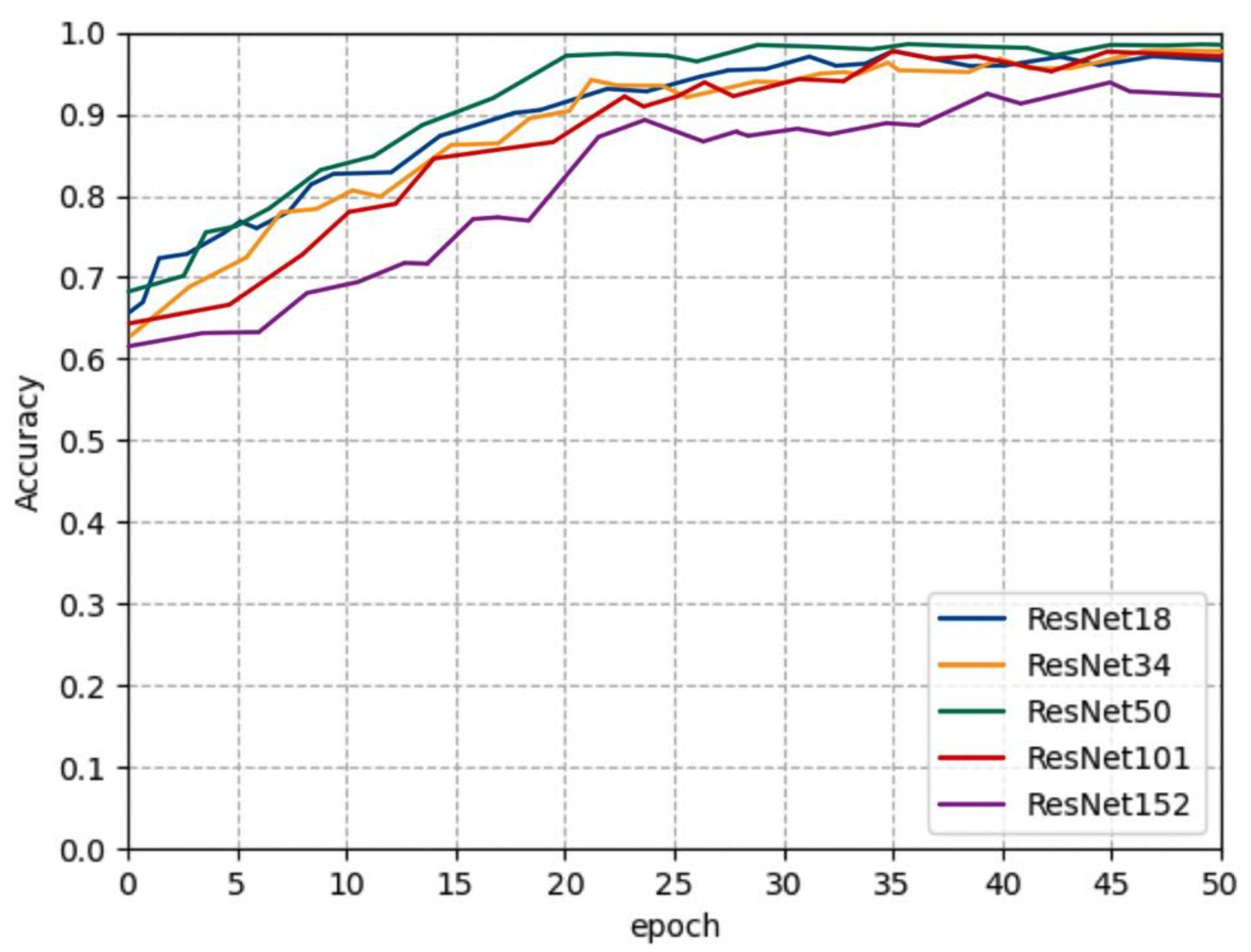
Through experiments, it is found that ResNet50 achieves the best performance where its accuracy on the test set was as high as 97.35%, as shown in Figure 10 and Table 3. The accuracy of the other two models was similar, (ResNet34 and ResNet101), reaching 96.81%, both higher than the rest. It adequately illuminates the powerful learning ability of the residual neural network. The accuracy of the model proposed in this paper can meet the requirements of pear defect detection in factories.
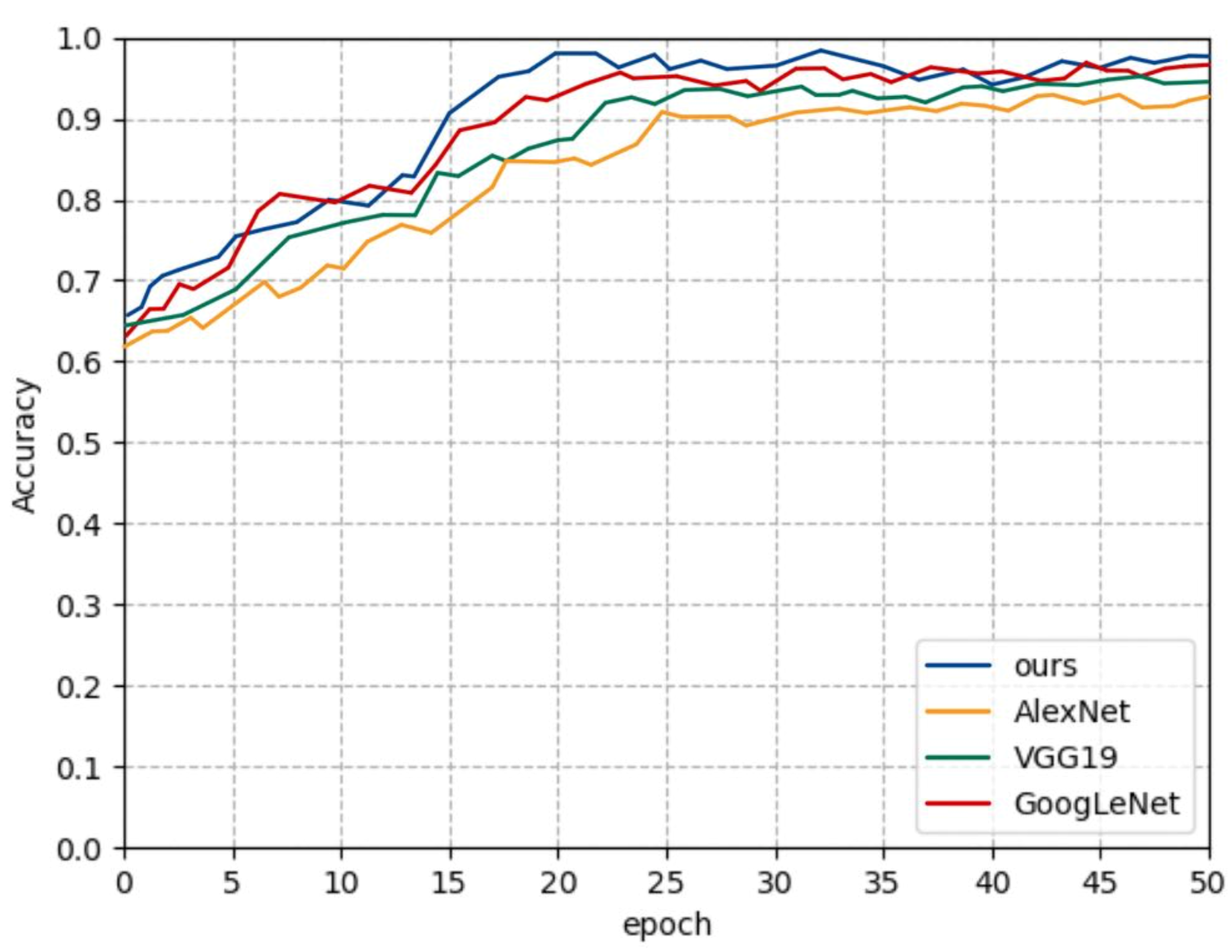
3.2. Comparison of CNN Models and Our Proposed Model
3.3. Comparison of Traditional ML Models and Ours
This paper picked three traditional machine learning models to conduct comparative experiments, including the support vector machine (SVM), random forests (RF) [30], and K-nearest neighbor (KNN) [31], whose cluster center is set to 2. Then the effectiveness and efficiency of our model were validated using the above-mentioned processed datasets and 10-fold validation. [25] The experimental results are shown in Table 5.
The accuracy of our model was 97.35%, which fully indicated that it is characterized by solid generalization capability and robustness. Concerning the other three traditional machine learning models, the support vector machine achieved an accuracy of 91.26% on the test set, the best performance among them. In conclusion, the experimental results revealed that ResNet50 transfer learning based on DCGAN has the best accuracy in the experiment with the superior structure. Meanwhile, the deep convolutional neural network can make end-to-end learning possible and reduce the time for manual feature extraction. It is efficient and effortless to operate, which is beneficial to the industrial production of factories.
4. Discussion
This paper validated the effectiveness of the model and tested its timing-based performance. The experimental results expounded that when the trained ResNet50 is utilized for inference, it takes 7–10 s to infer 100 images, meeting the production requirements.
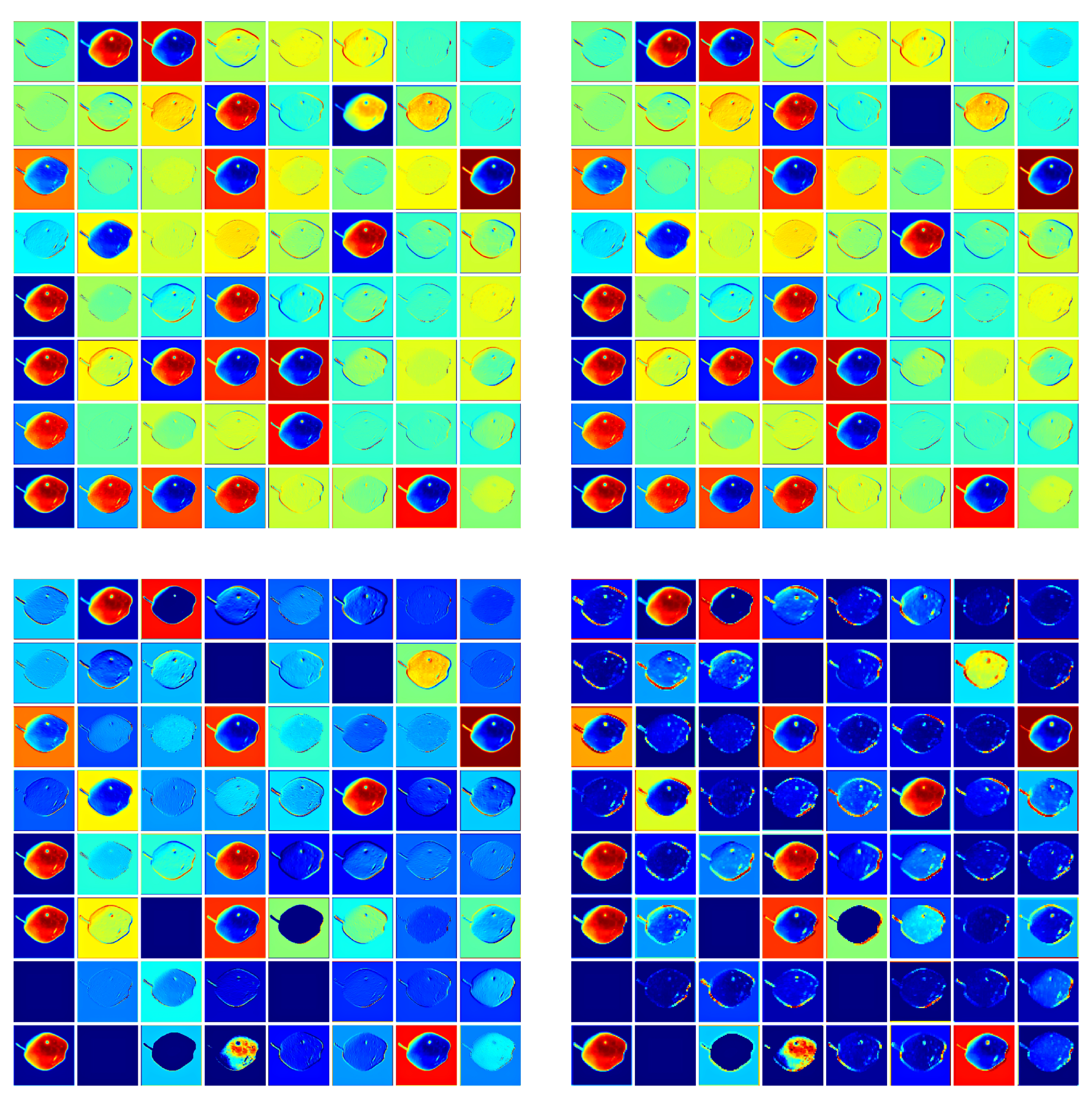
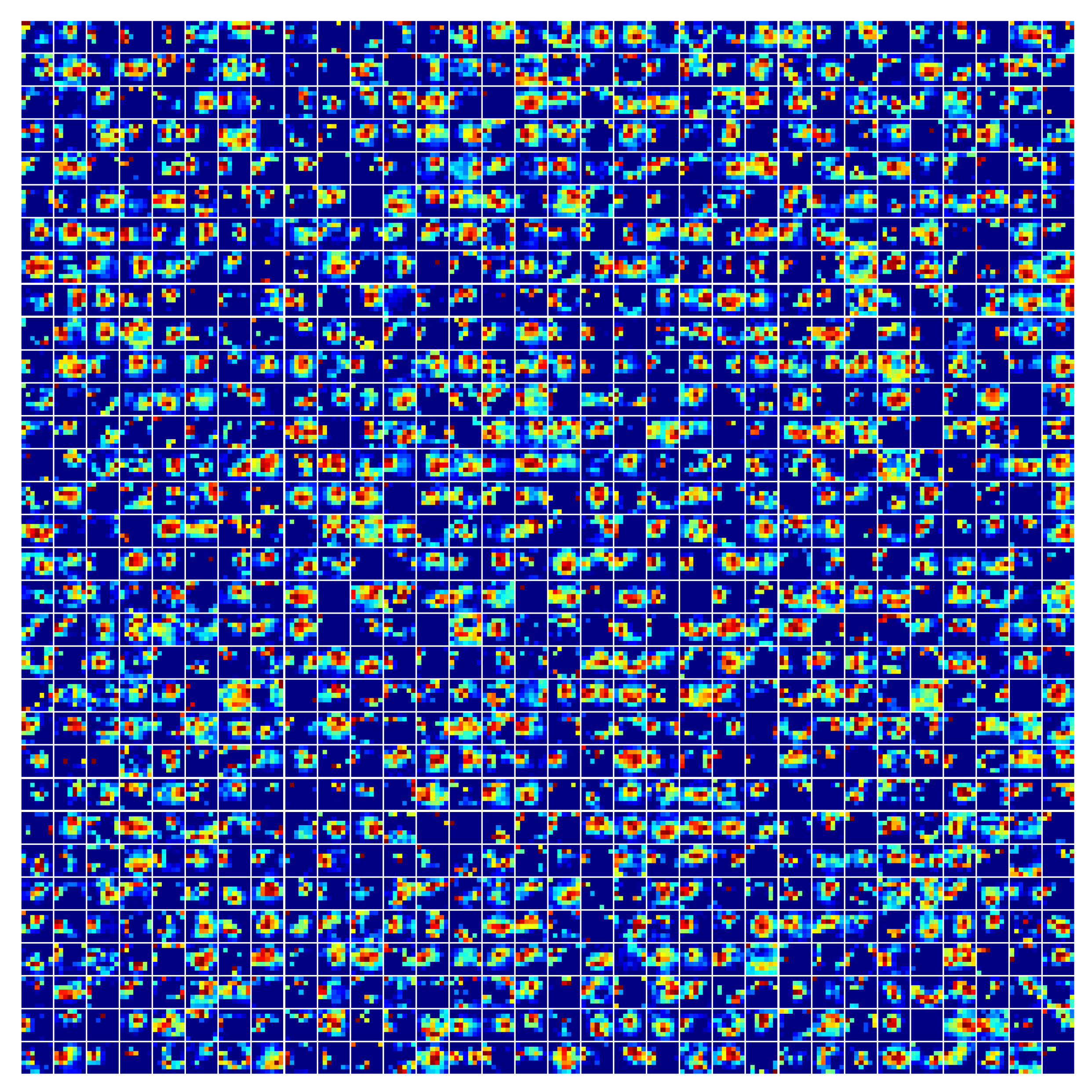
4.1. Visualization of Feature Map
The multi-channel feature maps, the output of ResNet50, were visualized with the highest accuracy in the experiment [32], as shown in Figure 12 and Figure 13. As can be seen from the figure, in the shallow layer feature maps, ResNet50 successfully extracted the lesion information of defective features. Even in Figure 13, the corresponding relationship between the highlighted color block area of the feature map and the defective feature in the original image can still be observed, which further proves the effectiveness of our model.
4.2. Ablation Experiments to Verify the Effectiveness of DCGAN
This paper carried out a comparative ablation experiment to validate the effectiveness of DCGAN-generated data. This paper adopted Cutmix [33] and Mosaic [34] methods to extend data on the original data set (the control group without data extending), avoiding data extending caused by adopting the DCGAN method. The number of processed data set is identical among the three methods. The processed results were introduced to the ResNet50 and SVM methods. Experimental results reflected that the accuracy of ResNet50 and SVM models is considerably improved when using the DCGAN method, with the best performance. Meanwhile, the accuracy of the DCGAN method was higher than that of the control group and the two other methods. The results are shown in Table 6.
4.3. Model Generalization Capability Validation
In order to verify the generalization capability of our model, ResNet50 model was selected from the above models and tested on two pear varieties that have not been trained before. As shown in Table 7, the experimental results show that our method is excellent.
4.4. Intelligent Pear Defect Detection System
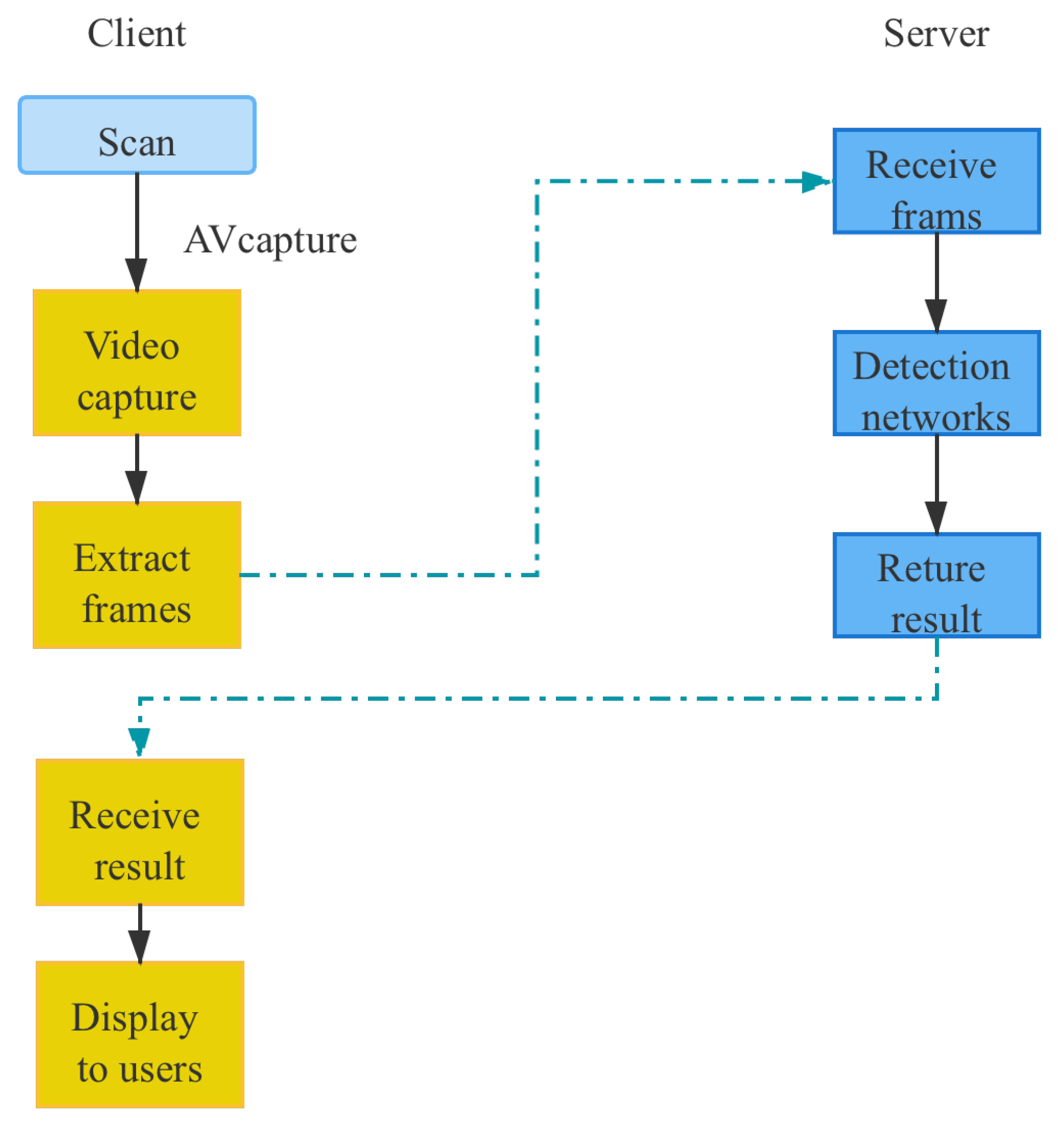
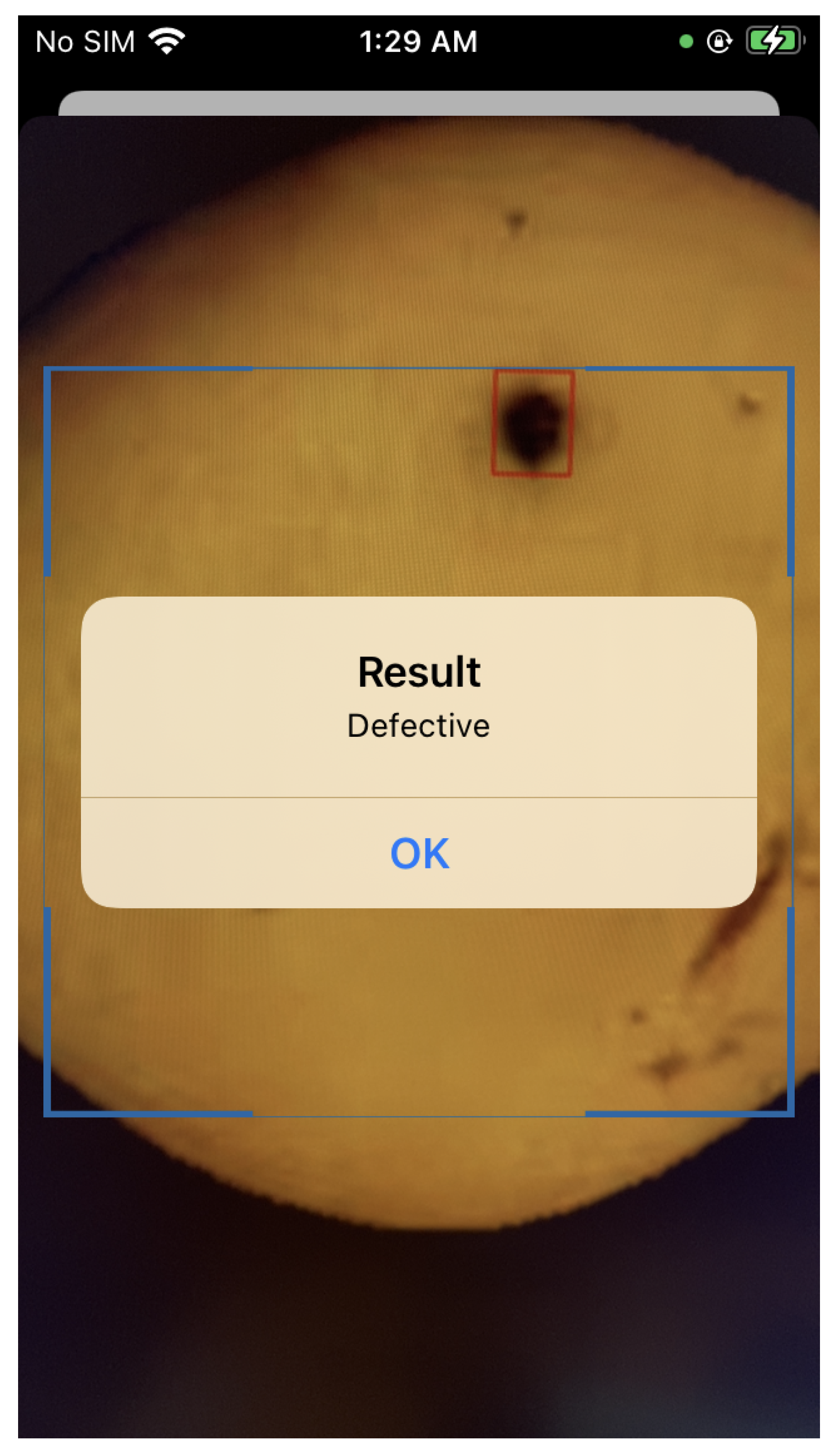
In order to realize the end-to-end mode of pear defect detection, and enable the model proposed in this paper to be applied to the agricultural production environment, an intelligent pear defect detection system on iOS based on Swift was developed. The workflow of the system is shown in Figure 14.
First, we obtain the video input stream from the iPhone camera. Then, frames are extracted and sent to the server. After that, the server transfers the received images to the model proposed in this paper. Finally, the recognition result is returned to the client. A screenshot of this system is shown in Figure 15.
4.5. Experimental Conclusions
With each index higher than traditional machine learning methods and other CNN models, the proposed model modified from ResNet50 has achieved outstanding performance in pear defect detection, living up to industry standards in both effectiveness and timeliness.
5. Conclusions
In this paper, a small number of negative samples were augmented by a deep convolutional generative adversarial network, and transfer learning was carried out by ResNet afterwards. The accuracy of pear defect detection was 97.35% in the validation set, which was visibly higher than traditional machine learning algorithms. To validate the robustness of the model, two pear varieties that have never been trained were tested, namely Shanxi bergamot pear and Dangshansu pear (Pyrus Bretschneider Rehd). The accuracy of the model can still reach 97.11%. The experimental results demonstrated that the proposed method has remarkable generalization capability and robustness.
From the perspective of pear defect detection industrialization, if the experimental method and process we proposed were introduced, the figure of negative samples needed to construct the deep learning model will notably dwindle, and the industrial cost will be cut consequentially.
Author Contributions
Conceptualization, Y.Z. and S.W.; methodology, P.S.; validation, Y.Z., S.W. and P.S.; writing—original draft preparation, Y.Z.; writing—review and editing, Y.Z.; visualization, Y.Z.; supervision, Y.W.; project administration, Y.Z.; funding acquisition, Y.W. All authors have read and agreed to the published version of the manuscript.
Funding
This work was supported by the Beijing Nunicipal Natural Science Foundation Youth Project (5214026), the 2115 Talent Development Program of China Agricultural University.
Institutional Review Board Statement
Not applicable.
Informed Consent Statement
Not applicable.
Data Availability Statement
Not applicable.
Acknowledgments
We are grateful to the ECC of CIEE in China Agricultural University for their strong support during our thesis writing.
Conflicts of Interest
The authors declare no conflict of interest.
Abbreviations
The following abbreviations are used in this manuscript:
| DCGAN | Deep convolutional generative adversarial networks |
| CNN | Convolutional neural network |
| SVM | Support vector machines |
| RF | Random forest |
| KNN | K-nearest neighbor |
| ML | Machine learning |
| AUC | Area under curve |
References
- Zhang, S.; Xie, Z. Current status, trends, main problems and the suggestions on development of pear industry in China. In Journal of Fruit Science; Magazines Publishing House: New York, NY, USA, 2019; Volume 36, pp. 1067–1072. [Google Scholar]
- Tanaka, S.H. Stucdies on black spot disease of the Japanese Pear (Pirus serotina Rehd). In Memoirs of the College of Agriculture; Number 28; Kyoto University: Kyoto, Japan, 1933. [Google Scholar]
- Jackel, L.; Lecun, Y.; Stenard, C.; Strom, B.; Sharman, D.; Zuckert, D. Optical character recogntion for automatic teller machines. In Industrial Applications of Neural Networks; World Scientific: Singapore, 1998; pp. 375–378. [Google Scholar]
- Krizhevsky, A.; Sutskever, I.; Hinton, G. ImageNet Classification with Deep Convolutional Neural Networks. Adv. Neural Inf. Process. Syst. 2012, 25, 1097–1105. [Google Scholar] [CrossRef]
- El-Sawy, A.; El-Bakry, H.; Loey, M. CNN for Handwritten Arabic Digits Recognition Based on LeNet-5; Springer International Publishing: Basel, Switzerland, 2016. [Google Scholar]
- Zhaoyong, Z.; Dongjian, H.; Haihui, Z.; Yu, L.; Dong, S.; Ketao, C. Non-Destructive Detection of Moldy Core in Apple Fruit Based on Deep Belief Network. Food Sci. 2017, 38, 304–310. [Google Scholar]
- Simonyan, K.; Zisserman, A. Very Deep Convolutional Networks for Large-Scale Image Recognition. arXiv 2014, arXiv:1409.1556v6. [Google Scholar]
- He, K.; Zhang, X.; Ren, S.; Sun, J. Deep Residual Learning for Image Recognition. In Proceedings of the 2016 IEEE Conference on Computer Vision and Pattern Recognition (CVPR), Las Vegas, NV, USA, 27–30 June 2016. [Google Scholar]
- Szegedy, C.; Vanhoucke, V.; Ioffe, S.; Shlens, J.; Wojna, Z. Rethinking the Inception Architecture for Computer Vision. In Proceedings of the 2016 IEEE Conference on Computer Vision and Pattern Recognition (CVPR), Las Vegas, NV, USA, 27–30 June 2016; pp. 2818–2826. [Google Scholar]
- Huang, G.; Liu, Z.; Laurens, V.; Weinberger, K.Q. Densely Connected Convolutional Networks. In Proceedings of the IEEE Conference on Computer Vision and Pattern Recognition (CVPR), Honolulu, HI, USA, 21–26 July 2017. [Google Scholar]
- Hearst, M.; Dumais, S.; Osman, E.; Platt, J.; Scholkopf, B. Support vector machines. IEEE Intell. Syst. Appl. 1998, 13, 18–28. [Google Scholar] [CrossRef] [Green Version]
- Tian, H.; Wang, T.; Liu, Y.; Qiao, X.; Li, Y. Computer vision technology in agricultural automation—A review. Inf. Process. Agric. 2020, 7, 1–19. [Google Scholar] [CrossRef]
- Gomes, J.F.S.; Leta, F.R. Applications of computer vision techniques in the agriculture and food industry: A review. Eur. Food Res. Technol. 2012, 235, 989–1000. [Google Scholar] [CrossRef]
- Patrício, D.I.; Rieder, R. Computer vision and artificial intelligence in precision agriculture for grain crops: A systematic review. Comput. Electron. Agric. 2018, 153, 69–81. [Google Scholar] [CrossRef] [Green Version]
- Chen, X.; Guo, C.; Zhang, C.; Liu, Z.; Jiang, H.; Lou, B.; He, Y. Visual detection study on early bruises of Korla pear based on hyperspectral imaging technology. Guang Pu Xue Yu Guang Pu Fen Xi = Guang Pu 2017, 37, 150–155. [Google Scholar] [PubMed]
- Jinhe, Z.; Futang, P. A Method of Selective Image Graying. Comput. Eng. 2006, 20, 198–200. [Google Scholar]
- Chen, S.; Haralick, R.M. Recursive erosion, dilation, opening, and closing transforms. IEEE Trans. Image Process. 1995, 4, 335–345. [Google Scholar] [CrossRef] [PubMed]
- Gil, J.Y.; Kimmel, R. Efficient dilation, erosion, opening, and closing algorithms. IEEE Trans. Pattern Anal. Mach. Intell. 2002, 24, 1606–1617. [Google Scholar] [CrossRef] [Green Version]
- Wand, M.P.; Schucany, W.R. Gaussian-based kernels. In Canadian Journal of Statistics; Wiley Online Library: Hoboken, NJ, USA, 1990; Volume 18, pp. 197–204. [Google Scholar]
- Radford, A.; Metz, L.; Chintala, S. Unsupervised representation learning with deep convolutional generative adversarial networks. arXiv 2015, arXiv:1511.06434. [Google Scholar]
- Goodfellow, I.J.; Pouget-Abadie, J.; Mirza, M.; Xu, B.; Warde-Farley, D.; Ozair, S.; Courville, A.; Bengio, Y. Generative Adversarial Networks. Adv. Neural Inf. Process. Syst. 2014, 3, 2672–2680. [Google Scholar] [CrossRef]
- Pan, S.J.; Yang, Q. A survey on transfer learning. IEEE Trans. Knowl. Data Eng. 2009, 22, 1345–1359. [Google Scholar] [CrossRef]
- Pateria, A.; Vyas, V.; Pratyush, M. Enhanced Image Capturing Using CNN, 1990. Int. J. Eng. Adv. Technol. 2019, 8, 320–324. [Google Scholar]
- He, K.; Zhang, X.; Ren, S.; Sun, J. Delving Deep into Rectifiers: Surpassing Human-Level Performance on ImageNet Classification. In Proceedings of the CVPR, Santiago, Chile, 7–13 December 2015. [Google Scholar]
- Blum, A.; Kalai, A.; Langford, J. Beating the hold-out: Bounds for k-fold and progressive cross-validation. In Proceedings of the Twelfth Annual Conference on Computational Learning Theory, Santa Cruz, CA, USA, 7–9 July 1999; pp. 203–208. [Google Scholar]
- Bottou, L. Stochastic Gradient Descent Tricks. In Neural Networks: Tricks of the Trade; Springer: Berlin/Heidelberg, Germany, 2012. [Google Scholar]
- Cutkosky, A.; Mehta, H. Momentum improves normalized sgd. In Proceedings of the International Conference on Machine Learning, PMLR, Virtual, 13–18 July 2020; pp. 2260–2268. [Google Scholar]
- Abdullahi, H.S.; Sheriff, R.; Mahieddine, F. Convolution neural network in precision agriculture for plant image recognition and classification. In Proceedings of the 2017 Seventh International Conference on Innovative Computing Technology (INTECH), Luton, UK, 16–18 August 2017; IEEE: Piscataway, NJ, USA, 2017; Volume 10. [Google Scholar]
- Jurman, G.; Riccadonna, S.; Furlanello, C. A Comparison of MCC and CEN Error Measures in Multi-Class Prediction; Public Library of Science: San Francisco, CA, USA, 2012. [Google Scholar]
- Breiman, L. Random forest. Mach. Learn. 2001, 45, 5–32. [Google Scholar] [CrossRef] [Green Version]
- Peterson, L.E. K-nearest neighbor. Scholarpedia 2009, 4, 1883. [Google Scholar] [CrossRef]
- Cristea, P.D. Application of neural networks in image processing and visualization. In GeoSpatial Visual Analytics; Springer: Berlin/Heidelberg, Germany, 2009; pp. 59–71. [Google Scholar]
- Yun, S.; Han, D.; Oh, S.J.; Chun, S.; Choe, J.; Yoo, Y. Cutmix: Regularization strategy to train strong classifiers with localizable features. In Proceedings of the IEEE/CVF International Conference on Computer Vision, Seoul, Korea, 27 October–3 November 2019; pp. 6023–6032. [Google Scholar]
- Ge, Z.; Liu, S.; Wang, F.; Li, Z.; Sun, J. Yolox: Exceeding yolo series in 2021. arXiv 2021, arXiv:2107.08430. [Google Scholar]
Figure 1.
All amplified images corresponding to a single image.

Figure 2.
Image comparison before and after image grayscale processing.

Figure 3.
Processing of dilation and erosion.

Figure 4.
Image comparison before and after the opening operation of the defective pear (kernel coefficients are 1, 3, 6, 9 respectively).
Figure 4.
Image comparison before and after the opening operation of the defective pear (kernel coefficients are 1, 3, 6, 9 respectively).

Figure 5.
A 100 dimensional uniform distribution z is projected and reshaped.

Figure 6.
Flow chart of generative adversarial networks.

Figure 7.
Schematic diagram of residual structure.

Figure 8.
Two blocks in ResNet series diagrams: the left is BasicBlock and the right is Bottleneck.

Figure 9.
Schematic diagram of ResNet18.

Figure 10.
Training process of ResNet series.

Figure 11.
Training process of CNN models.

Figure 12.
Visualization of shallow feature maps.

Figure 13.
Visualization of deep feature map.

Figure 14.
Intelligent pear defect detection system flow chart.

Figure 15.
Screenshot on iPhone SE.


Table 1.
Dataset details distribution.
| Normal Pears | Defective Pears | |
|---|---|---|
| Original data | 1500 | 500 |
| After data augmentation | 13,500 | 6750 |
| Training set | 12,150 | 6075 |
| Validation set | 1350 | 675 |
Table 2.
The number of blocks in each layer of ResNet series.
| ResNet18 | ResNet34 | ResNet50 | ResNet101 | ResNet152 | |
|---|---|---|---|---|---|
| Blocks | 2, 2, 2, 2 | 3, 4, 6, 3 | 3, 4, 6, 3 | 3, 4, 23, 3 | 3, 8, 36, 3 |
Table 3.
Performance comparison of ResNet series models.
| ResNet18 | ResNet34 | ResNet50 | ResNet101 | ResNet152 | |
|---|---|---|---|---|---|
| Accuracy | 96.03% | 96.81% | 97.35% | 96.17% | 92.96% |
| Precision | 0.961 | 0.974 | 0.973 | 0.953 | 0.917 |
| MCC | 0.854 | 0.859 | 0.863 | 0.861 | 0.819 |
Table 4.
Comparison of CNN models and our proposed model.
| Ours | AlexNet | VGG19 | GoogLeNet | |
|---|---|---|---|---|
| Accuracy | 97.35% | 92.25% | 94.88% | 96.04% |
| Precision | 0.973 | 0.927 | 0.943 | 0.958 |
| MCC | 0.863 | 0.848 | 0.851 | 0.859 |
Table 5.
Comparison of traditional ML models and ours.
| Ours | SVM | RF | KNN | |
|---|---|---|---|---|
| Accuracy | 97.35% | 91.26% | 87.14% | 73.29% |
| Precision | 0.973 | 0.919 | 0.851 | 0.741 |
| MCC | 0.863 | 0.829 | 0.733 | 0.591 |
Table 6.
Comparison of the models’ accuracy between using DCGAN and other situations.
| DCGAN | Cutmix | Mosaic | Without Data Extending | |
|---|---|---|---|---|
| ResNet50 | 97.35%(ours) | 95.71% | 96.93% | 95.37% |
| SVM | 91.26% | 88.31% | 91.14% | 88.39% |
Table 7.
Accuracy of detection of two pear varieties that have not been trained on the model.
| Shanxi Bergamot Pear | Dangshansu Pear | |
|---|---|---|
| Accuracy | 97.11% | 96.73% |
Publisher’s Note: MDPI stays neutral with regard to jurisdictional claims in published maps and institutional affiliations. |
© 2021 by the authors. Licensee MDPI, Basel, Switzerland. This article is an open access article distributed under the terms and conditions of the Creative Commons Attribution (CC BY) license (https://creativecommons.org/licenses/by/4.0/).
Share and Cite
MDPI and ACS Style
Zhang, Y.; Wa, S.; Sun, P.; Wang, Y. Pear Defect Detection Method Based on ResNet and DCGAN. Information 2021, 12, 397. https://0-doi-org.brum.beds.ac.uk/10.3390/info12100397
AMA Style
Zhang Y, Wa S, Sun P, Wang Y. Pear Defect Detection Method Based on ResNet and DCGAN. Information. 2021; 12(10):397. https://0-doi-org.brum.beds.ac.uk/10.3390/info12100397
Chicago/Turabian StyleZhang, Yan, Shiyun Wa, Pengshuo Sun, and Yaojun Wang. 2021. "Pear Defect Detection Method Based on ResNet and DCGAN" Information 12, no. 10: 397. https://0-doi-org.brum.beds.ac.uk/10.3390/info12100397
Note that from the first issue of 2016, this journal uses article numbers instead of page numbers. See further details here.