Financial Volatility Forecasting: A Sparse Multi-Head Attention Neural Network

Abstract

Accurately predicting the volatility of financial asset prices and exploring its laws of movement have profound theoretical and practical guiding significance for financial market risk early warning, asset pricing, and investment portfolio design. The traditional methods are plagued by the problem of substandard prediction performance or gradient optimization. This paper proposes a novel volatility prediction method based on sparse multi-head attention (SP-M-Attention). This model discards the two-dimensional modeling strategy of time and space of the classic deep learning model. Instead, the solution is to embed a sparse multi-head attention calculation module in the network. The main advantages are that (i) it uses the inherent advantages of the multi-head attention mechanism to achieve parallel computing, (ii) it reduces the computational complexity through sparse measurements and feature compression of volatility, and (iii) it avoids the gradient problems caused by long-range propagation and therefore, is more suitable than traditional methods for the task of analysis of long time series. In the end, the article conducts an empirical study on the effectiveness of the proposed method through real datasets of major financial markets. Experimental results show that the prediction performance of the proposed model on all real datasets surpasses all benchmark models. This discovery will aid financial risk management and the optimization of investment strategies.

1. Introduction

Finance is the core of the modern economy, and economic and financial globalization has exacerbated the generation, exposure, spillover, and contagion of financial market risks. The prediction of financial volatility plays an important role in studying financial risk management, asset pricing, and investment portfolio theory. Improving the accuracy of volatility forecasts, prompting decision-makers to decide on expected changes in advance, is of great significance to maintaining the stability of the financial market and improving investment returns. With the continuous development of computer technology, the ability to acquire and use financial market transaction data is increasing, and more asset price information can be used in research and practice. This type of data contains richer market information and can reflect the price fluctuations of financial assets. In the past 40 years, many scholars at home and abroad have carried out a significant amount of research work around volatility prediction, exploring the law of fluctuations in financial asset prices. Among them are classic time series forecasting models based on the law of large numbers and central limit theory, including the autoregressive model (AR), random walk model (RW), moving vector autoregressive model (ARIMA), etc. However, these models have strong assumptions about the constant variance of price fluctuation data and cannot effectively model the “spike”, “fat tail”, and “clustering” characteristics of volatility changes that reflect the complexity of the time series of financial volatility.

In 1982, Engle [1] first proposed the conditional heteroscedasticity (ARCH) model, which is an econometric model developed on the basis of the AR model, abandoning the ideal assumption that variance is constant. This model has a more powerful ability to fit and explain financial time series and has been widely used in financial time series analysis. However, the characteristics of ARCH inevitably produce a large number of parameters to be estimated and consume significant computational resources, which limits the popularity of the model. In 1986, Bollerslev [2] added the variance lag term of the ARCH model and creatively proposed generalized autoregressive conditional heteroscedasticity (GARCH) to improve the universality of the model. Subsequently, many variants or combinations of models based on GARCH have been proposed and widely used in financial volatility prediction and risk measurement [3,4,5,6]. F Klaassen [7] (2002) proposed the Markov regime-switching GARCH model to achieve multi-cycle volatility forecasts for the United States dollar. Abdalla and SZ Suliman [8] (2012) used GARCH to forecast currency exchange rate volatility. P Agnolucci [9] (2009) compared the predictive performance of the GARCH and implied volatility models using West Texas Intermediate Oil contract data. Nelson Daniel, B. (1992) examined the relation between stock returns and stock market volatility. They found evidence of a negative correlation between current returns and future returns and proposed the exponential general autoregressive conditional heteroskedastic (EGARCH) model [10].

Compared to GARCH, the stochastic volatility (SV) method can better describe the characteristics of financial price fluctuations and has good statistical characteristics. Melino, Turnbull, and Stuart M. [11] (1990) studied the impact of stochastic volatility on spot foreign currency option pricing and proposed a method of exchange rate diffusion with stochastic volatility to price foreign currency options and compare their pricing with observed market prices. Tse [12] (1991) used the stochastic volatility method to model and predict the volatility of the Japanese stock market, and through experiments proved that the stochastic volatility method (SV) is better than GARCH in the Asian market. Mariani et al. [13] (2018) proposed a random volatility method that relies on filtering techniques and compared it with GARCH. The results show that SV is a better forecasting tool than GARCH (1,1). Suk-Joon Byun, Sol Kim, Dongwoo Rhee [14] (2009) suggested using SV to predict future volatility from option prices.

The model of stochastic volatility (SV) improves the generalization ability of data by adding extra white noise to the variance equation, but this extra feature makes it difficult to estimate the SV model accurately, which restricts the application of the model. The realized volatility (RV) theory, proposed by Anderson [15] (2003), is another widely studied theory about modeling financial volatility. Compared to GARCH, SV, and other traditional models, this theory can reflect the macroscopic and microscopic information on volatility more fully. Moreover, it overcomes the shortcoming of the traditional model. There are many modeling methods based on the RV theory. Among them, Corsi, Audrino, and Renò [16] (2012) proposed the different value regression realized volatility (HAR-RV), which has attracted wide interest among scholars. This method calculates the average realized volatility of the day, week, or month, and obtains the corresponding realized volatility of the day, week, or month. Based on the HAR model, Qu and Ji [17] proposed an adaptive heterogeneous autoregressive (AHAR) model to optimize the original HAR model by genetic algorithm to adapt to the market with different time structures. The model can automatically adjust the structure and actively adapt to changes as the market changes over time. In addition, the model also characterizes the typical characteristics of high-frequency financial data such as long-term memory, peaks, and thick tails, and can use least squares estimation, so it has a wide range of application scenarios [18].

In recent decades, intelligent prediction technology represented by machine learning has made breakthroughs. It has powerful processing capabilities for massive, high-dimensional, high-noise, non-linear, and non-stationary data, so it has been widely used in the field of financial data analysis. Among the machine learning methods that can be used to predict volatility, especially the support vector machine [19] and neural network [20] methods are the most popular. SAH A and ZI B [21] (2004) applied the artificial neural network method to volatility prediction through the futures options pricing model. After comparing with the implied volatility of S&P 500 index futures options, they found that they were based on an artificial neural network. The forecasting performance is better than the implied volatility, and there is no significant difference between the predicted value and the actual volatility. LBTang, LXTang, and HYSheng [22] (2019) believed that conventional support vector machines could not accurately describe the aggregation phenomenon of stock market return volatility, and proposed a wavelet kernel function SVM, namely WSVM, and used real data to evaluate the model. Applicability and effectiveness are verified.

Kristjanpoller and Minutolo [23] (2016) proposed a hybrid model based on the combination of artificial neural networks and GARCH and applied it to the prediction of crude oil price volatility. E. Ramos-Pérez et al. [24] (2019) stack multiple machine learning methods such as random forest, support vector machine, and artificial neural network into a combined model. The experimental results of the volatility of the S&P500 index show that the model has higher prediction accuracy than the baseline method.

Deep learning is the most important subset of machine learning. It not only has made great achievements in pattern recognition and natural language processing but also has been widely used in the financial field. Many traditional complex problems have been solved with great breakthroughs [25]. LSTM [26] is a deep learning model that can analyze time-series data and has long-term memory ability and nonlinear fitting ability. At present, it has been used by many scholars to forecast financial asset price volatility. Kim and Won [27] put forward the GEW-LSTM model based on the combination of LSTM and GARCH. All of the MSE, MAE, and HMSE show that GEW-LSTM is better than the advanced forecasting methods.

Liu, Y. [28] (2019) used a long and short-term memory recurrent neural network (LSTM) to conduct a series of volatility prediction experiments. Experimental results show that this method is better than classical GARCH (SVM) prediction results, which benefit from the powerful data fitting ability of deep learning. Traditional deep learning methods such as LSTM and GRU have a long memory capacity, but the remote valuable information is transmitted to the current node in a hidden state with a lag time sequence. The longer the transmission distance, the more information is forgotten, and the risk of mission failure increases. Bahdanau, Cho, and Bengio [29] (2014) introduced the attention mechanism to neural networks for the first time, so that the model can capture and lock important information and improve the accuracy of machine translation. Since then, the attention mechanism has been continuously improved and has gradually become one of the mainstream technologies of natural language processing [30]. Google (2017, Ashish Vaswani et al. [31]) further proposed a deep learning model, transformer, based on a new self-attention mechanism, which has better output quality and more effective parallelism than previous machine translation methods.

LSTM and GRU add gate mechanisms based on RNN, but they are still recurrent neural networks in essence. In other words, the state of the nodes in such networks depends on the hidden information about the previous time step. Although the gate control mechanism alleviates the problem of gradient explosion and disappearance to some extent, it cannot completely solve the above problems. Furthermore, the recurrent neural network can only transfer information sequentially, which affects the speed of the model. Transformer realizes parallel computing, but there are many problems such as too many waiting parameters, quadratic time complexity, and large memory consumption, which limit its application for long time series analysis tasks. Zhou, Zhang [32] (2020) presents the Informer model, which is a variant based on the transformer. It includes a self-attention mechanism called ProbSparse. This mechanism uses a sparse mechanism to reduce the input feature information and the parameters to be learned by halving step by step, which effectively reduces the quadratic time complexity of LSTF tasks. Experiments on such datasets as electricity consumption showed that the performance of Informer is significantly better than that of the existing methods and provides a new solution to the LSTF problem.

The most significant contribution of our work is the proposal of a sparse multi-head attention (SP-M-Attention) based volatility prediction model, which draws inspiration from the design of transformer and Informer. This novel approach uses an encoder-decoder architecture. It makes full use of the parallel processing mechanism of multi-head attention to capture complex features, achieving the goal of improving the efficiency of data fitting. However, the problem of gradient disappearance during the learning of long-term autocorrelated features still cannot be solved if we rely on multiple attentions alone. Hence, we then introduced the approximate sparse measure in the multi-head attention module to obtain a sparse representation of the query. Subsequently, we could then compute the prediction results with relatively few key queries. As can be seen from the above description, the method makes full use of the sparse characteristics of financial volatility sequences and achieves learning and prediction of long-term memory features of volatility sequences without sacrificing prediction accuracy. Compared to traditional methods, this novel model is more effective for volatility prediction tasks with long-memory, non-stationary features, and significantly improves prediction accuracy.

The rest of this article is arranged as follows. Section 2 is related to the work, summarizing the preliminary related research, introducing some relevant technical background, and research strategy. Section 3 describes the core modules of the proposed approach. Section 4 presents the layout of experiments and evaluates the results. Finally, Section 5 summarizes the work of this paper.

2. Related Work

Volatility forecasting research is an active branch of finance research, and many methods have emerged in the last decades. However, none of these methods is perfect, and all of them have some insurmountable shortcomings in terms of model structure, estimation methods, and applicability. For example, the GARCH family models require a numerical balance between the degree of random factor shocks and the degree of volatility persistence, which makes it difficult to capture sudden and large fluctuations in financial markets during the estimation of GARCH-type models. In addition, the descriptive and predictive power of GARCH-type models depends heavily on the type of distribution of the stochastic disturbance term ε, which reduces the usefulness of GARCH-type models. The non-linear relationship between unobservable log volatility and returns in SV models makes the calculation and modeling of the likelihood function extremely difficult. RV has a strong volatility portrayal capability, but in the estimation stage of the model, the sampling frequency cannot obtain a consistent standard, which hinders the construction of a reasonable model. The heterogeneous autoregressive (HAR) model combines volatility components of different frequencies to capture heterogeneous market participant types, and although it is highly analytical, the complex structure of the data makes the model inadequate in characterizing certain features [33]. The above approaches based on traditional statistics or econometrics, which usually rely on linear regression, do not achieve the desired accuracy of prediction when the explanatory variables are strongly correlated or exhibit low signal-to-noise ratios, or when the data structure presents a high degree of nonlinearity. In contrast, general machine learning and deep learning algorithms rely on big data-driven and supervised learning methods with strong data-fitting superiority, but remain inadequate in areas such as learning of fine-grained and long-memory features.

Recent studies show that deep learning, especially recurrent neural networks, is the most effective method to predict volatility. RNN can learn the autocorrelation features of time series, but the risk of gradient disappearance or explosion increases with the increase in the length of the input series. This defect limits the learning of long sequence dependence and long-term memory features for recurrent neural network models. LSTM and GRU, which are variants of RNN, adjust the transmission and storage of information by gate control structure, to some extent reducing the negative effect of gradient problems. However, they do not solve the problem of long-term memory of information because of all RNN family models passing information in order. The state and output of each time node depend on the state of the previous history node, not just the current input. At present, LSTM mainly adopts the strategy of multi-layer stacking to capture long-term time-series features. The longer the time series interval and the more LSTM stack layers, the longer the path of information transmission will be. This situation increases the risk of information loss and reduces the model’s predictive performance.

The attention model draws on human thought patterns. It can directly learn the dependence between any two objects in time or space, ignoring the Euclidean distance. This advantage can help observers to quickly capture high-value information. The self-attention mechanism is a type of special attention that describes the autocorrelation of time series variables. It relies less on external information and is better at capturing the internal autocorrelation of time series data. Therefore, it has been applied in natural language processing and time series analysis.

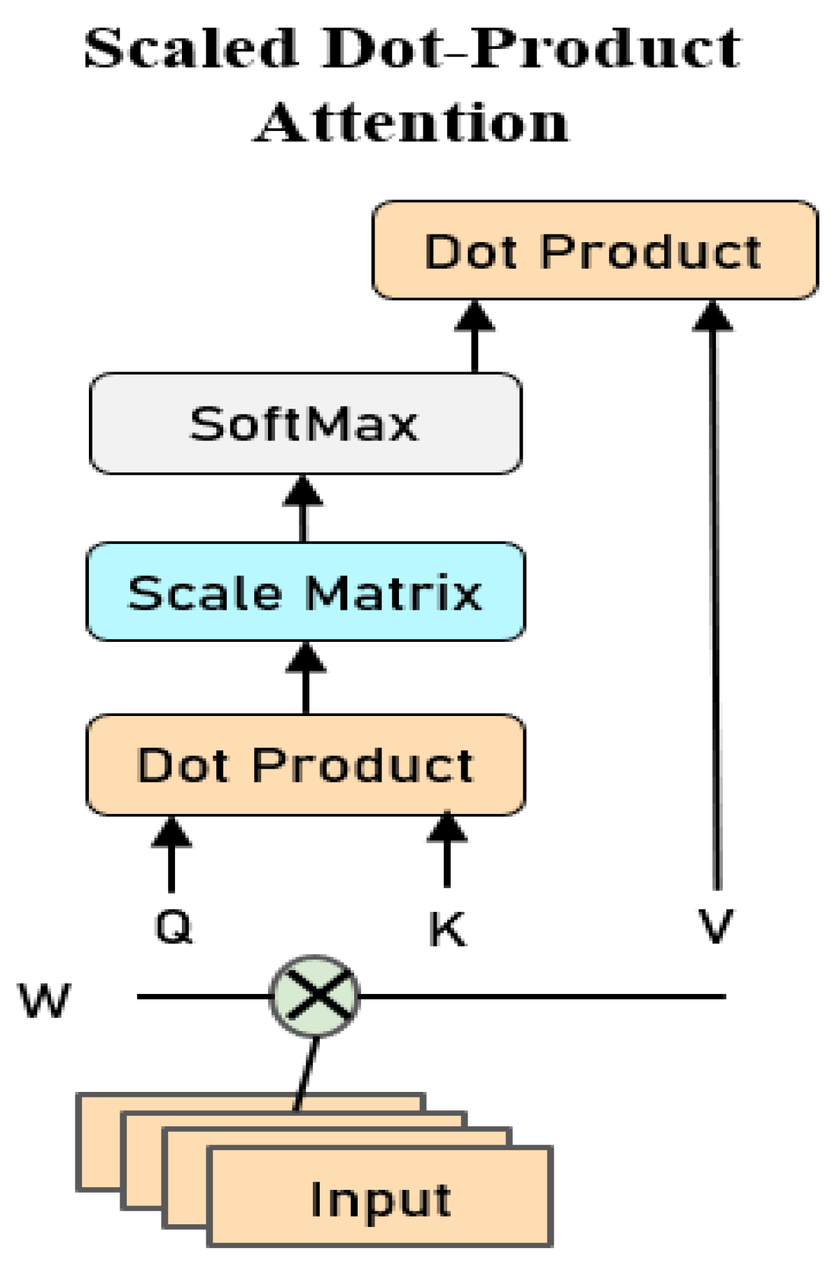
The essence of the attention mechanism is the process of focusing on important information or addressing it. Given a query vector q related to the task, calculate the probability distribution of the attention for each Key, and multiply it by the value to obtain the attention score. A typical self-attention framework named scaled dot-product attention is shown in Figure 1:

Step 1: In the embedding layer, we convert each input ${\mathrm{X}}_{:,\mathrm{t}}$ to a feature vector X with dimension d, where ${\mathrm{X}}_{:,\mathrm{t}}={\left\{{\mathrm{x}}_{1,\mathrm{t}},{\mathrm{x}}_{2,\mathrm{t}},\dots ,{\mathrm{x}}_{\mathrm{N}-1,\mathrm{t}},\dots {\mathrm{x}}_{\mathrm{N},\mathrm{t}}\right\}}^{\mathrm{T}}\in {ℝ}^{\mathrm{N}\times 1}$, which is the observation vector of N time series at the t-th time step.

Step 2: Multiply the embedding vector X by the weight matrix ${\mathrm{W}}^{\mathrm{Q}}\in {ℝ}^{\mathrm{d}\times {\mathrm{L}}_{\mathrm{k}}}$, ${\mathrm{W}}^{\mathrm{K}}\in {ℝ}^{\mathrm{d}\times {\mathrm{L}}_{\mathrm{K}}}$, ${\mathrm{W}}^{\mathrm{V}}\in {ℝ}^{\mathrm{d}\times {\mathrm{L}}_{\mathrm{V}}}$.

$$\mathrm{Q}=\mathrm{X}·{\mathrm{W}}^{\mathrm{Q}},\mathrm{K}=\mathrm{X}·{\mathrm{W}}^{\mathrm{K}},\mathrm{V}=\mathrm{X}·{\mathrm{W}}^{\mathrm{V}}$$

(1)

This is a linear transformation of the embedded vector process. K and Q make up the key-value combination, so ${\mathrm{W}}^{\mathrm{Q}}$ and ${\mathrm{W}}^{\mathrm{K}}$ have the same dimensions.

Step 3:$\frac{\mathrm{Q}{\mathrm{K}}^{\mathrm{T}}}{\sqrt{{\mathrm{d}}_{\mathrm{k}}}}$. Given the time cost and space efficiency of the calculations, we preferred scaled dot-product attention. Multiply $\mathrm{Q}{\mathrm{K}}^{\mathrm{T}}$ by scaling factor $\frac{1}{\sqrt{{\mathrm{d}}_{\mathrm{k}}}}$, so that the gradient can be kept stable, and the solution process can be correctly converged until the optimal solution is obtained. If the result after dot multiplication is too large, the gradient may fall into a very small region when the adjustment of the parameter propagates backward.

Step 4:$\mathrm{softmax}\left(\frac{\mathrm{Q}{\mathrm{K}}^{\mathrm{T}}}{\sqrt{{\mathrm{d}}_{\mathrm{k}}}}\right)$. Convert the vector to a probability distribution that has a range of [0, 1] and a sum of 1. The probability here can be understood as the weight multiplied by the value V.

Step5: Calculate and obtain the weighted attention score $\mathrm{Attention}(\mathrm{Q},\mathrm{K},\mathrm{V})$ of each input vector. This score determines the contribution of each input to the current location label.

$$\mathrm{Attention}(\mathrm{Q},\mathrm{K},\mathrm{V})=\mathrm{softmax}\left(\frac{\mathrm{Q}{\mathrm{K}}^{\mathrm{T}}}{\sqrt{{\mathrm{d}}_{\mathrm{k}}}}\right)\mathrm{V}$$

(2)

The SP-M-Attention model proposed in the next section of this paper is a special attention mechanism that has been improved and optimized to fit our problem.

3. Methodology

3.1. Problem Discussion

We will build an efficient forecasting model to capture the autocorrelation characteristics of volatility and the correlation with N-1 other time series at medium-grain or fine-grain. The input $\mathrm{X}=\left\{{\mathrm{X}}_{:,0,}{\mathrm{X}}_{:,1,}\dots ,{\mathrm{X}}_{:,\mathrm{t}},\dots \right\}$, where ${\mathrm{X}}_{:,\mathrm{t}}={\left\{{\mathrm{x}}_{1,\mathrm{t}},{\mathrm{x}}_{2,\mathrm{t}},\dots ,{\mathrm{x}}_{\mathrm{N}-1,\mathrm{t}},\dots {\mathrm{x}}_{\mathrm{N},\mathrm{t}}\right\}}^{\mathrm{T}}\in {ℝ}^{\mathrm{N}\times 1}$. X is a multivariate time series consisting of the predicted series itself and other N-1 auxiliary time series. Our goal is to predict the future values of volatility based on the observed historical data of the N correlated time series. It can be described by Equation (3).

$$\left\{{\mathrm{X}}_{:,\mathrm{t}+1},{\mathrm{X}}_{:,\mathrm{t}+2},\dots ,{\mathrm{X}}_{:,\mathrm{t}+\tau }\right\}={\mathrm{F}}_{\mathsf{\theta }}({\mathrm{X}}_{:,\mathrm{t}},{\mathrm{X}}_{:,\mathrm{t}-1},\dots ,{\mathrm{X}}_{:,\mathrm{t}-\mathrm{T}+1})$$

(3)

where θ denotes all the learnable parameters in model training, $\mathrm{F}(·)$ denotes the proposed model, and τ denotes the τ-step ahead prediction.

3.2. Sparse Multi-Head Self-Attention

3.2.1. Multi-Head Self-Attention

A single self-attention maps a query and a key into the same high-dimensional space to compute similarity, capturing only a limited set of dependencies on the timing data. However, a complex time series often has multiple dependencies. On the other hand, multi-head self-attention can describe the autocorrelation of different levels of subspaces in the sequence in parallel. Multifarious attention allows the model to focus on the characteristics of different levels of subspaces in time series and capture the dependencies on different time positions. Therefore, it has a more outstanding data representation ability than a single attention structure.

$$\mathrm{Multi}-\mathrm{head}(\mathrm{Q},\mathrm{K},\mathrm{V})=\mathrm{Concat}({\mathrm{head}}_1,{\mathrm{head}}_2,\cdots {\mathrm{head}}_{\mathrm{h}})·{\mathrm{W}}^{\mathrm{o}}$$

(4)

$${\mathrm{head}}_1=\mathrm{Attention}\left(\mathrm{Q}{\mathrm{W}}_{\mathrm{i}}^{\mathrm{Q}},\mathrm{K}{\mathrm{W}}_{\mathrm{i}}^{\mathrm{K}},\mathrm{V}{\mathrm{W}}_{\mathrm{i}}^{\mathrm{V}}\right)$$

(5)

where ${\mathrm{W}}_{\mathrm{i}}^{\mathrm{Q}}\in {ℝ}^{{\mathrm{d}}_{\mathrm{model}}\times {\mathrm{d}}_{\mathrm{k}}},{\mathrm{W}}_{\mathrm{i}}^{\mathrm{K}}\in {ℝ}^{{\mathrm{d}}_{\mathrm{moodel}}\times {\mathrm{d}}_{\mathrm{k}}},{\mathrm{W}}_{\mathrm{i}}^{\mathrm{V}}\in {ℝ}^{{\mathrm{d}}_{\mathrm{model}}\times {\mathrm{d}}_{\mathrm{v}}}$, ${\mathrm{W}}^{\mathrm{O}}\in {ℝ}^{\mathrm{h}{\mathrm{d}}_{\mathrm{v}}\times {\mathrm{d}}_{\mathrm{model}}}$.

The projection is the parameter matrix ${\mathrm{W}}_{\mathrm{i}}^{\mathrm{Q}}$, ${\mathrm{W}}_{\mathrm{i}}^{\mathrm{K}}$, ${\mathrm{W}}_{\mathrm{i}}^{\mathrm{V}}$. In practice, we perform multiple dot-product attention computations on input X in parallel to obtain multiple intermediate outputs. These intermediate output results are then spliced together. To keep the dimensions unchanged, we multiply the result by a weight matrix. We used h attention headers and then use an extra attention head ${\mathrm{head}}_{\mathrm{i}}$ to integrate all the attention and output. Since the dimension of each head is reduced, the total computational cost is similar to that of single head attention.

3.2.2. Sparse Self-Attention

The self-attention mechanism can arbitrarily model the sequence autocorrelation relationship. Each self-attention layer has a global receptive domain and can assign characterization capabilities to the most valuable features. Therefore, the neural network using this architecture is more flexible than the sequential connection mode network. However, this type of network also has its shortcomings, one of which is that the demand for memory and computing power increases twice as the sequence length increases. Therefore, the computational overhead limits its application in long-memory time series.

Because the probabilistic distribution of attention is sparse, the distribution of attention per query over all keys is far from uniform. The sparse representation characterizes the signal as much as possible with a small number of parameters, which helps to reduce computational and storage complexity. SP-M-Attention takes advantage of Informer’s sparse representation scheme and reduces computational complexity by limiting the number of query-key pairs [32]. The relative entropy method is used to measure the similarity of the probability distribution of queries and keys. Thus, the dot-product of the dominant top-n query-key is selected. The sparse high-dimensional signals in the original wave series are simplified into low-dimensional subspaces. The function of this operation is not only to ensure the effectiveness of training and learning but also to reduce the data noise and the complexity of computation and storage.

Suppose the i-th query’s attention to all keys is defined as a probability ${\mathrm{p}(\mathrm{k}}_{\mathrm{j}}{|\mathrm{q}}_{\mathrm{i}})$. From scaled dot-product attention, we can deduce ${\mathrm{p}(\mathrm{k}}_{\mathrm{j}}{|\mathrm{q}}_{\mathrm{i}})={\displaystyle \sum _{\mathrm{j}=1}^{\mathrm{d}}\frac{{\mathrm{q}}_{\mathrm{i}}{\mathrm{K}}_{\mathrm{j}}^{\mathrm{T}}}{\sqrt{{\mathrm{d}}_{\mathrm{k}}}}}$. Then, an algorithm called relative entropy is used to measure the “similarity” between queries Q and keys K and filter out the important queries. The relative entropy of the i-th query can be expressed as follows:

$$\mathrm{D}\left(\overline{\mathrm{q}}\left|\right|\mathrm{p}\right)=\ln \sum _{\mathrm{j}=1}^{{\mathrm{L}}_{\mathrm{K}}}{\mathrm{e}}^{\frac{{\overline{\mathrm{q}}}_{\mathrm{i}}{\mathrm{K}}_{\mathrm{j}}^{\top }}{\sqrt{\mathrm{d}}}}-\frac{1}{{\mathrm{L}}_{\mathrm{K}}}\sum _{\mathrm{j}=1}^{{\mathrm{L}}_{\mathrm{K}}}\frac{{\overline{\mathrm{q}}}_{\mathrm{i}}{\mathrm{K}}_{\mathrm{j}}^{\top }}{\sqrt{\mathrm{d}}}$$

(6)

Here, it is assumed that the attention $\overline{\mathrm{q}}$ of the i-th query ${\mathrm{Q}}_{\mathrm{i}}$ on all keys is uniformly distributed. ${\overline{\mathrm{q}}}_{\mathrm{i}}$ is the probability (weight) of the i-th query-key pair. Then ${\overline{\mathrm{q}}}_{\mathrm{i}}=1/{\mathrm{Q}}_{\mathrm{len}},\mathrm{i}\in \{1,2,\cdots {\mathrm{Q}}_{\mathrm{len}}\}$. If the i-th query-key pair obtains a larger $\mathrm{D}\left(\overline{\mathrm{q}}\left|\right|\mathrm{p}\right)$, it indicates that the attention of the i-th query ${\mathrm{Q}}_{\mathrm{i}}$ to all keys deviates from the uniform distribution, and the head of the long-tail self-attention distribution contains the dominant dot-product pair. The probability is higher.

However, measuring $\mathrm{D}\left(\overline{\mathrm{q}}\left|\right|\mathrm{p}\right)$ requires the calculation of each dot-product. Because the query has the same dimension as the key, that is ${\mathrm{L}}_{\mathrm{Q}}={\mathrm{L}}_{\mathrm{K}}$. The complexity is $\mathrm{O}({\mathrm{L}}_{\mathrm{Q}}{\mathrm{L}}_{\mathrm{K}})$ or $\mathrm{O}({\mathrm{L}}_{\mathrm{K}}^2)$. To reduce computational overhead, we apply an approximate query sparsity measure called maximum mean measurement.

From Equation (6), we can obtain:

$$\mathrm{D}\left(\overline{\mathrm{q}}\left|\right|\mathrm{p}\right)\le \underset{\mathrm{j}}{\max }\left\{\frac{{\overline{\mathbf{q}}}_{\mathrm{i}}{\mathbf{K}}_{\mathrm{j}}^{\top }}{\sqrt{\mathrm{d}}}\right\}-\frac{1}{{\mathrm{L}}_{\mathrm{K}}}\sum _{{\mathrm{L}}_{\mathrm{K}}}^{\mathrm{j}=1}\frac{{\overline{\mathbf{q}}}_{\mathrm{i}}{\mathbf{K}}_{\mathrm{j}}^{\top }}{\sqrt{\mathrm{d}}}$$

(7)

Then, the maximum mean value is:

$$\mathrm{M}\left(\overline{\mathrm{q}},\mathrm{p}\right)=\underset{\mathrm{j}}{\max }\left\{\frac{{\overline{\mathbf{q}}}_{\mathrm{i}}{\mathbf{K}}_{\mathrm{j}}^{\top }}{\sqrt{\mathrm{d}}}\right\}-\frac{1}{{\mathrm{L}}_{\mathrm{K}}}\sum _{{\mathrm{L}}_{\mathrm{K}}}^{\mathrm{j}=1}\frac{{\overline{\mathbf{q}}}_{\mathrm{i}}{\mathbf{K}}_{\mathrm{j}}^{\top }}{\sqrt{\mathrm{d}}}$$

(8)

Thus, in the case of sparse distribution of attention, we only need to randomly sample $\mathrm{N}={\mathrm{L}}_{\mathrm{Q}}\ln {\mathrm{L}}_{\mathrm{K}}$ pairs of queries and keys for dot-product calculations. Other positions in the sparse matrix are filled with zero values. Because the max operator in $\mathrm{M}(\overline{\mathrm{q}},\mathrm{p})$ is not sensitive to zero, the calculated value of $\mathrm{M}(\overline{\mathrm{q}},\mathrm{p})$ is stable. After optimization, the computational complexity is $\mathrm{O}\left({\mathrm{L}}_{\mathrm{Q}}\ln {\mathrm{L}}_{\mathrm{K}}\right)\le \mathrm{O}({\mathrm{L}}_{\mathrm{Q}}{\mathrm{L}}_{\mathrm{K}})$, which reduces the computational complexity and memory overhead.

Based on the approximate sparsity measure mentioned earlier, we obtain a sparse matrix composed of top-n pairs of predominant queries and keys. Finally, by multiplying the sparse matrix with V (Value), we obtain approximate self-attention scores:

$$\mathcal{A}(\overline{\mathbf{Q}},\mathbf{K},\mathbf{V})=\mathrm{Softmax}\left(\frac{\overline{\mathbf{Q}}{\mathbf{K}}^{\top }}{\sqrt{\mathrm{d}}}\right)\mathbf{V}$$

(9)

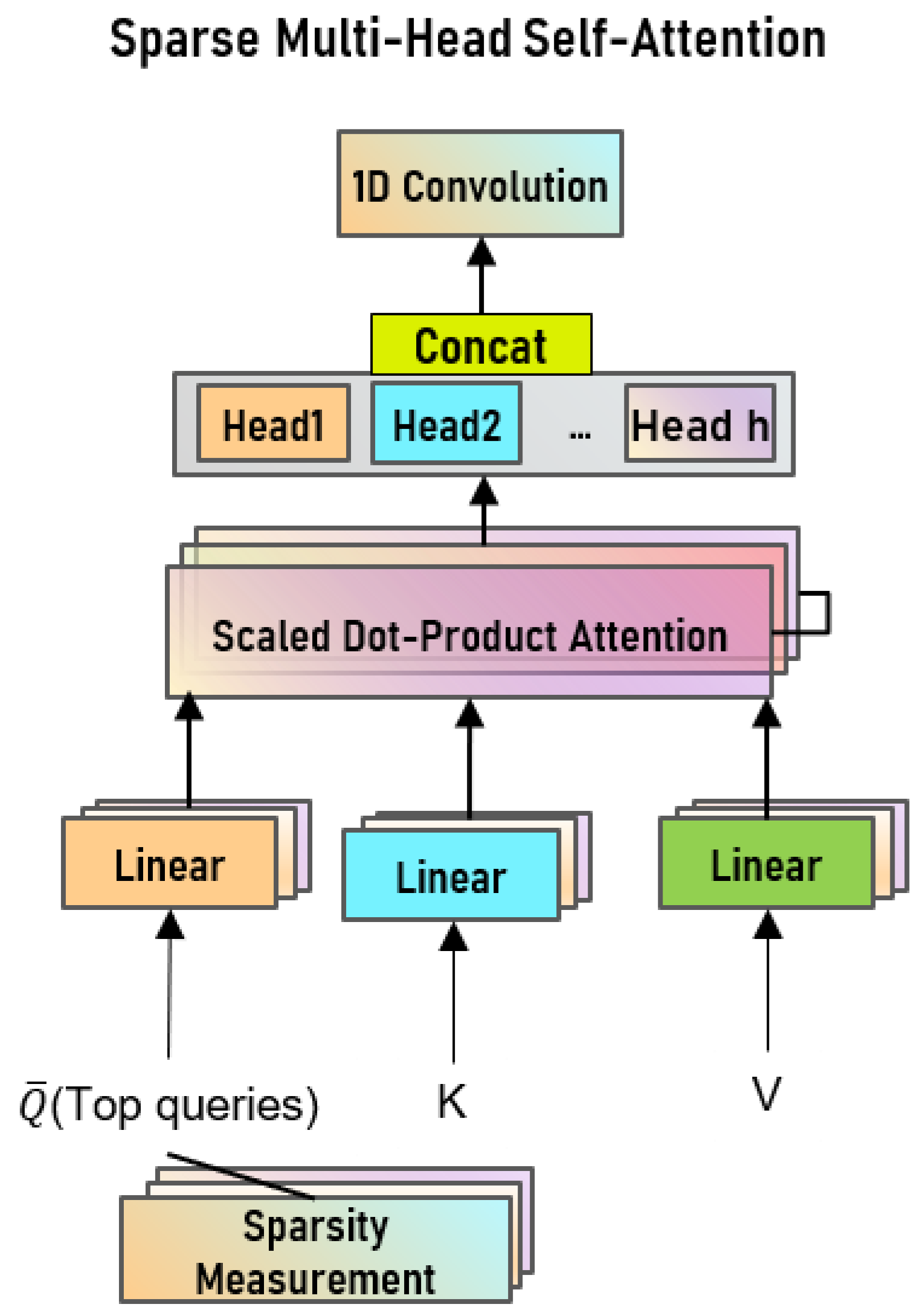
where, Q contains only the top-u queries after the sparse metric M (q, K). Figure 2 is a computational flowchart of multi-head sparse self-attention.

Sparse measurement is the compression of queries to obtain a sparse representation of the queries, i.e., a sparse matrix. An effective sparse representation not only ensures information quality but also reduces the computational complexity of model training. From Figure 2, we can easily observe that the multi-head attention module processes the input queries, keys, and values in a parallel manner, which is what makes it surpass the classical deep learning models LSTM and GRU. Not only that, although h attention heads are used, the total computational cost of all attention heads is similar to the full-dimensional single-head attention because the dimensionality of each head is reduced.

3.3. Model Architecture

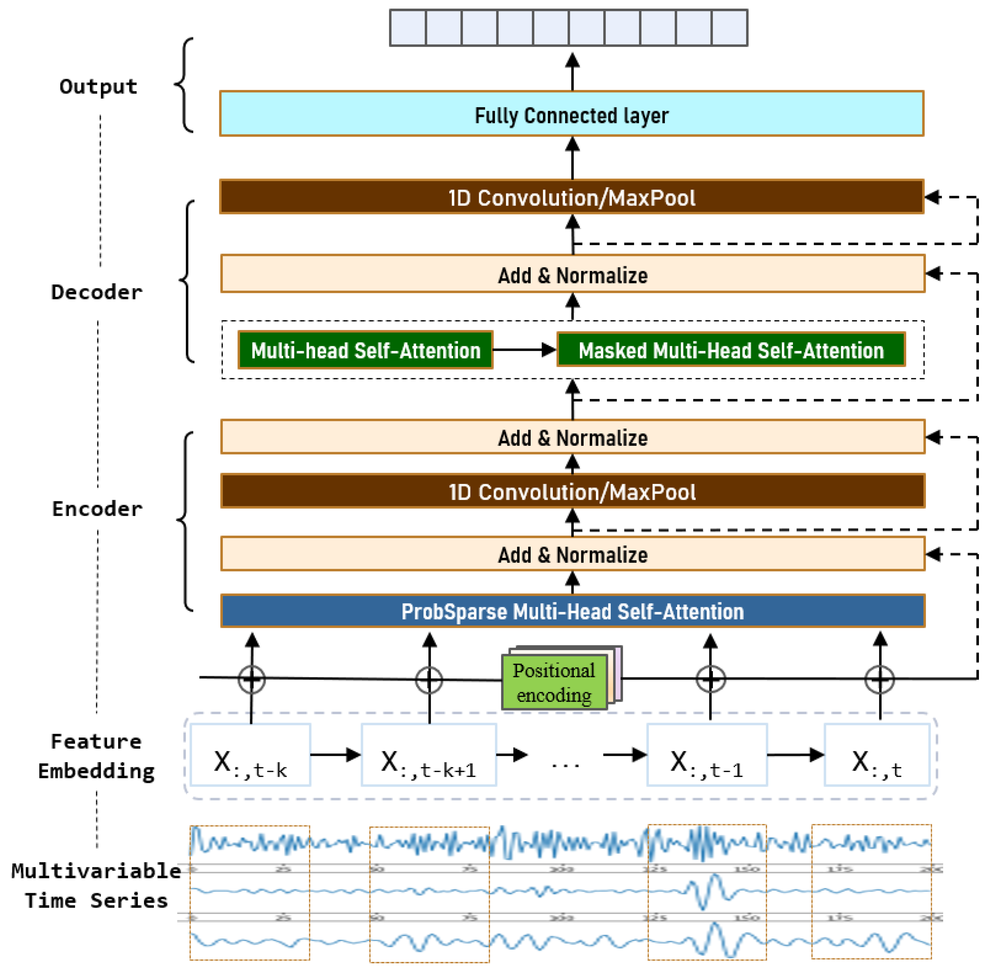
The self-attention model has been successfully used in the field of machine translation [34]. We propose an enhanced attention volatility model that uses the Encoder-Decoder architecture even though the data form is quite different from the former. Let us explain the structure of the proposed model in detail. The architecture is shown in Figure 3.

3.3.1. Encoder

Encoders can be stacked to obtain stronger data characterization capabilities. Each encoder includes two core sublayers. The first is the sparse multi-head self-attention layer, which is mainly responsible for the adaptive learning of data features. In the self-attention layer, all keys, values, and queries come from the output of the previous layer. The other core sublayer is a 1D convolutional neural network layer. In the encoder, the residual connection method is used between layers, and after each sub-layer, there is a normalization layer that plays an auxiliary role. Each position in the encoder can focus on all positions in the previous layer of the encoder.

3.3.2. Decoder

The decoder can also be stackable for performance enhancement. In addition to the two sublayers in the encoder layer, each decoder also has a masked multi-head self-attaching sublayer to prevent position i from noticing subsequent locations. This masking, combined with the fact that the output is embedded in a position offset, ensures that the prediction of position i depends only on known output less than position i.

3.3.3. 1D Convolution Neural Networks

Unlike feedforward neural networks in Transformer, encoders and decoders include 1D convolution neural networks in addition to the self-attention sublayer. A one-dimensional convolution neural network mainly deals with time series data and is often used in sequence models. The moving directions of convolution nuclei and pooled nuclei are one-dimensional. The translation invariance and parameter sharing of 1D convolution networks reduce the number of parameters that need to be learned.

3.3.4. Residual Connection and Normalization Layer

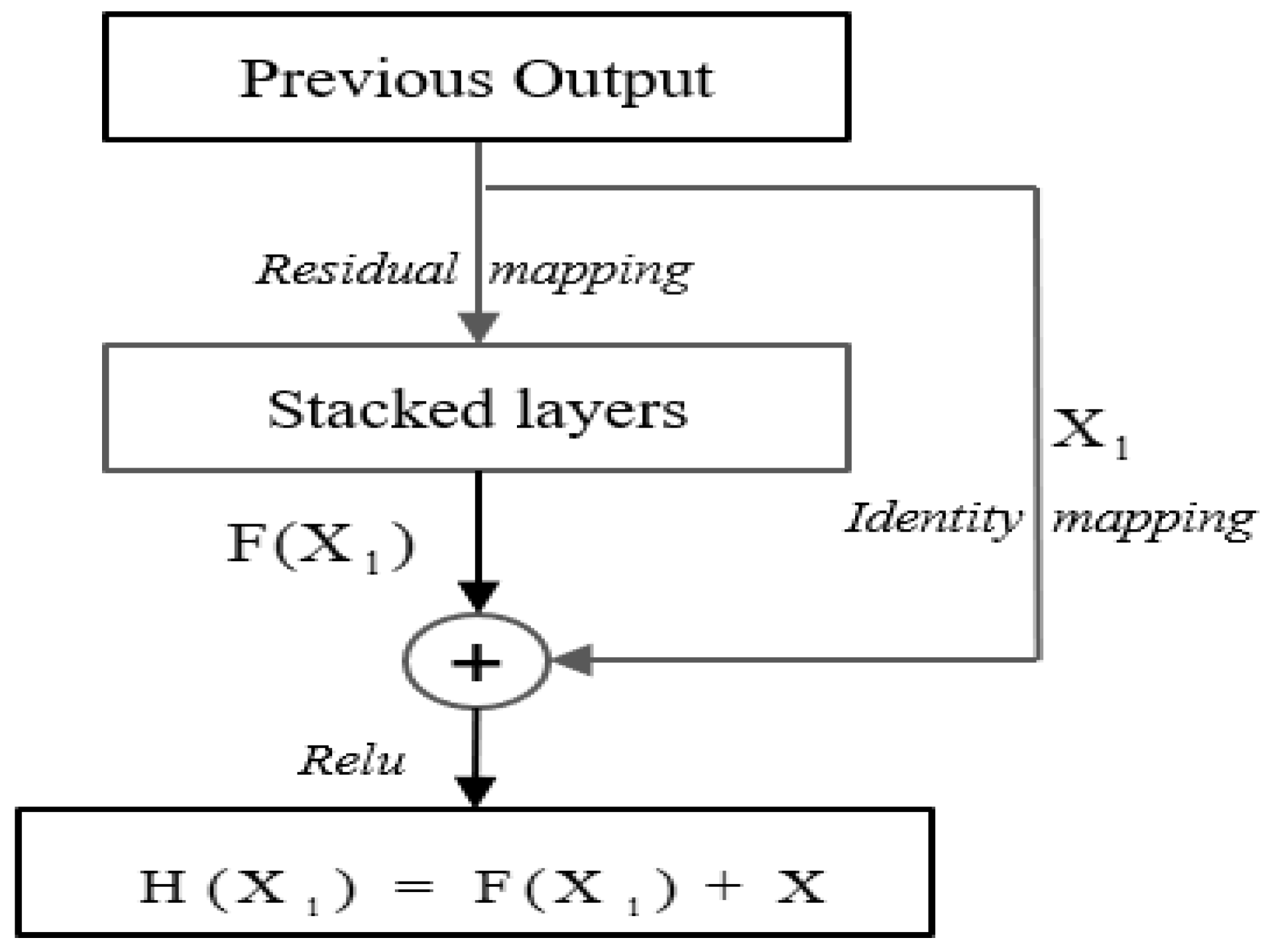
Encoder-Decoder is stacked with layers of neural networks. Theoretically, the deeper the neural network is, the stronger the ability to express data features is, and it seems easier to reduce the training error by increasing the network depth. In practice, however, adding more layers to the model at the appropriate depth can lead to a saturation of accuracy or even higher training errors. We call this phenomenon “degeneration”. To circumvent this type of risk, we use a residual connection between the network layers inside the Encoder-Decoder structure, so that the network output H(x) = F(x) + x. The structure of the residual connection is shown in Figure 4.

When the network is at its best, continue to deepen the networks, and the residual mapping will push to 0, leaving only the identity mapping. Therefore, in theory, the network is always in the optimal state, and the network performance does not decline with the increase in depth.

However, for deep neural networks, even if the input data has been standardized, the update of model parameters during training can still easily cause drastic changes in the output of the output layer. This instability of calculated values usually makes it difficult for us to train an effective depth model. Batch normalization is proposed to meet the challenge of deep model training. During model training, batch normalization uses the mean and standard deviation of the small batch to continuously adjust the intermediate output of the neural network, so that the value of the intermediate output of the entire neural network in each layer is more stable.

3.3.5. Embedding and Output

As with other sequence-to-sequence models, we use learning embedding to convert input and output tags into vectors. If it is a categorized task, enter the next token probability embedded in the model to convert the decoder output to a predicted value through linear transformations and activation functions. The volatility prediction is a regression task, so the output vector of the model represents the prediction result of the forward n-step.

3.3.6. Positional Encoding

The attention mechanism is different from classical deep learning models such as CNN, RNN, and LSTM with strict location information. During the transformation process of the multi-head self-attention module, the order of entries inside the input vectors will be disrupted. For our model to be able to take advantage of the position information in the original sequence, we added a “position encode” to the input embedding at the bottom of the encoder and decoder stack. Positional encoding and embedding have the same dimension d, so the two can be added. In this study, we use sine and cosine functions of different frequencies as position codes.

$$\begin{array}{l}{\mathrm{P}}_{(\mathrm{pos},2\mathrm{i})}^{\mathrm{encoder}}=\sin \left(\mathrm{pos}/{10000}^{2\mathrm{i}/\mathrm{d}}\right)\\ {\mathrm{P}}_{(\mathrm{pos},2\mathrm{i}+1)}^{\mathrm{encoder}}=\cos \left(\mathrm{pos}/{10000}^{2\mathrm{i}/\mathrm{d}}\right)\end{array}$$

(10)

where pos is the position and i is the dimension. That is, each dimension of the position code corresponds to a sine wave. We choose this function because we assume that it can make the model easy to learn by relative position. After all, for any fixed offset k, ${\mathrm{P}}_{\mathrm{pos}+\mathrm{k}}^{\mathrm{encoder}}$ can be expressed as a linear function of ${\mathrm{P}}_{\mathrm{pos}}^{\mathrm{encoder}}$.

4. Experiment

4.1. Dataset

In this study, three real financial datasets of Standard & Poor’s 500 Index (SPX500), West Texas Intermediate (WTI), and London Metal Exchange Gold Price (LGP) were used to verify the effectiveness of our proposed method. The Standard & Poor’s 500 Index (SPX500) represents the North American stock market. The daily data of West Texas Intermediate (WTI) crude oil prices represent oil prices. The LGP is the most influential precious metal price index.

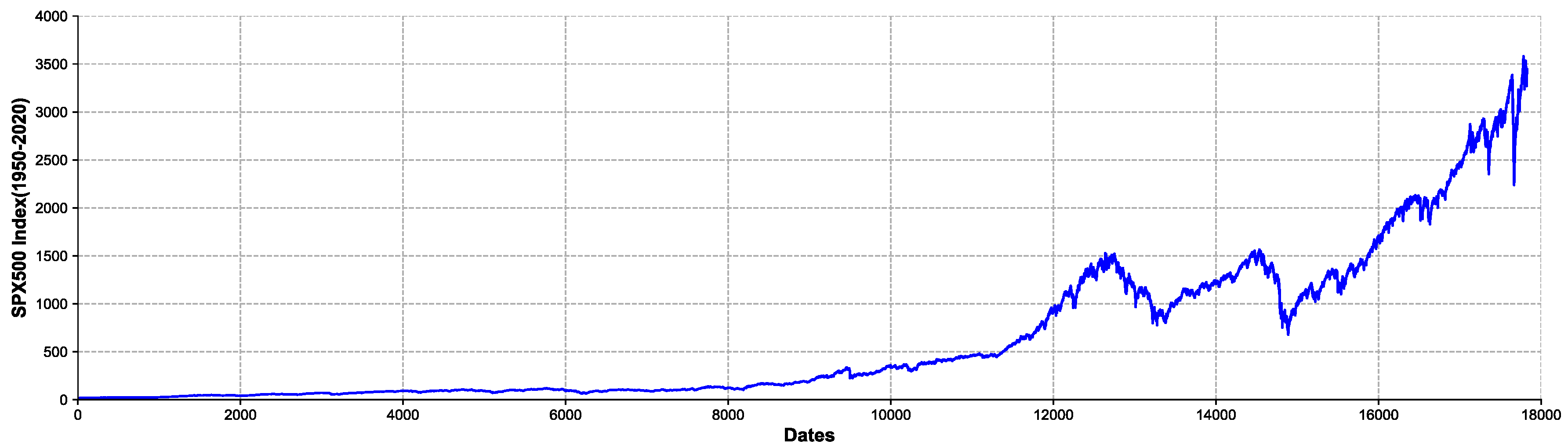
Take the SPX500 dataset as an example. The data coming from Yahoo! Samples are collected every minute from 3 January 1950, to 4 November 2020. The source dataset contains 17,827 observations, each of which contains the open, low, high, close, volume, and Adj close. Each feature constitutes an independent time series. In these series, we calculate the Adj close to obtain a continuous composite logarithmic rate of return and historical volatility. Figure 4 shows the trend of the SPX500 (1950–2020) index. From Figure 5, we can observe that the series has obvious nonlinear and wave aggregation characteristics.

Table 1. Descriptive statistics of log return.

Datasets	Mean	Std-Dev.	Skewness	Kurtosis	Jarque–Bera
SPX500	9.36 × 10−6	0.001525	−0.011905	20.75456	170,957.0
Oil	0.000180	0.022712	−0.540034	16.69873	62,169.60
Gold	0.000249	0.012181	0.062319	13.99408	66,698.44

shows us the descriptive statistics of the three datasets. The mean value of the log-return of the three datasets is all close to 0, which is significantly smaller than the corresponding standard error. The kurtosis of all the series is greater than 3, indicating that the three log-return series have obvious non-normal distribution and volatility agglomeration characteristics. The stock index and crude oil return series are left-skewed (skewness < 0), and their skewness differs from gold returns, which are positive. This reflects that stock market indexes and crude oil price return sequences are more volatile than gold prices. The kurtosis of all markets is above 3, that is, it has the characteristic of “high-peak” and “fat-tail” (kurtosis > 3), which shows that we cannot assume that the return distribution is normal. In addition, the Jarque–Bera test results also reject the normality hypothesis.

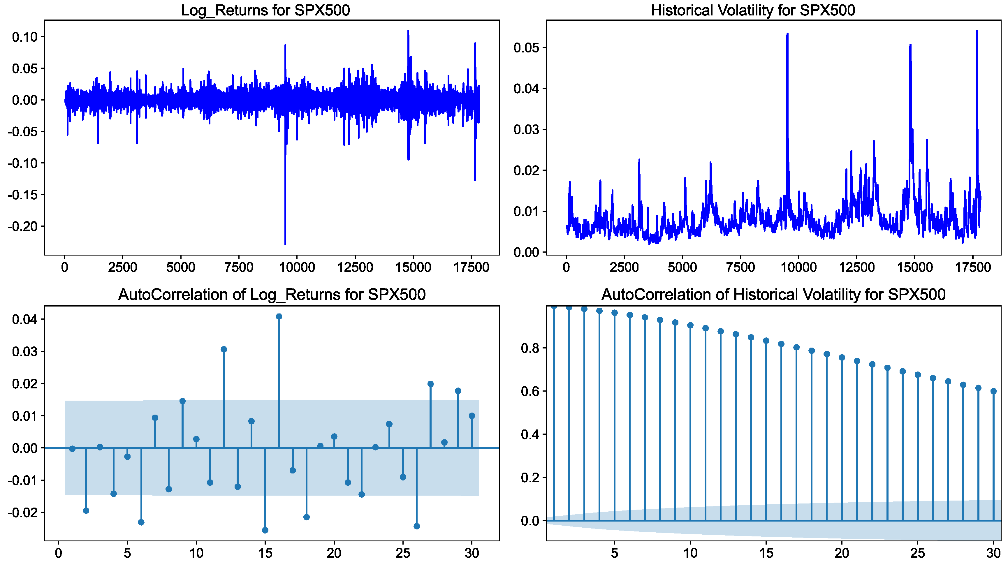
Figure 6 shows the log return, volatility, and autocorrelation of the SPX500 index. Volatility is defined as the deviation of asset returns from the mean. In this paper, we estimate volatility by calculating the standard deviation of log asset returns.

$${\mathrm{R}}_{\mathrm{i}}=\ln \left({\mathrm{S}}_{\mathrm{i}}\right)-\ln \left({\mathrm{S}}_{\mathrm{i}-1}\right)=\ln \left(\frac{{\mathrm{S}}_{\mathrm{i}}}{{\mathrm{S}}_{\mathrm{i}-1}}\right)$$

(11)

where ${\mathrm{R}}_{\mathrm{i}}$ denote the i-th log returns, ${\mathrm{S}}_{\mathrm{i}}$ is the asset price at the end of the i-th interval, and $\ln (·)$ is the natural logarithmic function.

$${\mathrm{V}}_{\mathrm{i}}=\sqrt{\frac{1}{\mathrm{N}-1}\sum _{\mathrm{i}=1}^{\mathrm{N}}{\left({\mathrm{R}}_{\mathrm{i}}-\overline{\mathrm{R}}\right)}^2}$$

(12)

$$\mathrm{V}=\{{\mathrm{V}}_0,{\mathrm{V}}_1,\cdots {\mathrm{V}}_{\mathrm{t}-1},{\mathrm{V}}_{\mathrm{t}}\}$$

(13)

where ${\mathrm{V}}_{\mathrm{i}}$ is the i-th volatility, V is the time series of volatility, and t is the length of V.

In the following experiments, we set windows of width 30 to calculate the standard deviation ${\mathrm{V}}_{\mathrm{i}}$ and historical volatility V. As can be seen from the left subgraph of Figure 6, the return sequence of stock indexes has obvious characteristics of volatility clustering. The autocorrelation function graph of the SPX500 index return sequence is truncated, which indicates it is a white noise sequence and does not have significant autocorrelation. The subgraph on the right side of Figure 6 shows that the autocorrelation function graph of the volatility has obvious tailing characteristics. We should reject the hypothesis that there is no autocorrelation in the volatility, i.e., accept that there are typical autocorrelation features in the volatility.

The Hurst exponent reflects the autocorrelation of time series, especially the long-term trend hidden in time series. The Hurst index is measured in terms of both V/S and R/S, which are generally considered more efficient and robust.

Table 2. Hurst exponent of volatility sequence.

Hurst Exponent	SPX500	WTI	Gold
t = 30	0.6440	0.6532	0.6486
t = 60	0.6501	0.6556	0.6503

shows the Hurst indices for the time windows 30 and 60. It can be seen that all the Hurst indices of the three series are greater than 0.6, which reflects the significant long-term memory of the above fluctuation series.

4.2. Baseline Methods

To evaluate the overall performance of our approach, we compared the proposed model with the widely used baseline and state-of-the-art models, including GARCH (1, 1), EGARCH (1, 1), SV, RV, HAR, SVR, and LSTM, as well as multiple combinatorial models of GW-LSTM, W-SVR, HAR-RV, etc.

For the SVR model in the baseline method, we selected the radial basis function as the kernel function (kernel = ‘rbf’) and set penalty parameters to 1.0 (C = 1.0). To evaluate the proposed model more fairly, all deep learning methods in SP-M-Attention and the baseline were unified using mean square error (MSE) as the loss function, and Adam function as the model optimizer. We set the batch size to 72, the learning rate to 0.1, and each neural network model trains 500 epochs. In the experiments of LSTM and GW-LSTM baseline models, we determined the number of neurons and other hyper-parameters in the hidden layer by grid search and pre-training. In this paper, all the experiments involving deep learning were performed and completed under the environment of Pytorch 1.7.0 and CUDA 10.1.

4.3. Metrics

In subsequent experiments, two popular metrics, mean absolute error (MAE) and mean squared error (MSE), were used to evaluate the performance of the model. Both MAE and MSE are often used to measure the deviation between observations and forecasting values in the task of machine learning models.

(1)

mean absolute error (MAE)

$$\mathrm{MAE}(\mathrm{y},\hat{\mathrm{y}})=\frac{1}{\mathrm{N}}{\displaystyle \sum _{\mathrm{i}=1}^{\mathrm{N}}\left|{\mathrm{y}}_{\mathrm{i}}-{\widehat{\mathrm{y}}}_{\mathrm{i}}\right|}$$

(14)

(2)

mean squared error (MSE)

$$\mathrm{MSE}(\mathrm{y},\widehat{\mathrm{y}})=\frac{1}{\mathrm{N}}{\displaystyle \sum _{\mathrm{i}=1}^{\mathrm{N}}{\left({\mathrm{y}}_{\mathrm{i}}-{\widehat{\mathrm{y}}}_{\mathrm{i}}\right)}^2}$$

(15)

where y denotes the observations, $\widehat{\mathrm{y}}$ is the prediction, and N is the number of samples. In practice, the smaller the values of these two metrics, the closer the predicted results are to the actual observations, that is, the higher the prediction accuracy.

(3)

Diebold–Mariano test (DM test)

$$\mathrm{DM}=\frac{\overline{\mathrm{d}}}{\sqrt{[{\widehat{\mathsf{\gamma }}}_{\mathrm{d}}(0)+2{\displaystyle \sum _{\mathrm{k}=1}^{\mathrm{h}-1}{\widehat{\mathsf{\gamma }}}_{\mathrm{d}}}(\mathrm{k})]/\mathrm{T}}}$$

(16)

where $\overline{\mathrm{d}}$ is the sample mean of the loss differential, ${\widehat{\mathsf{\gamma }}}_{\mathrm{d}}$ is the autocovariance, and $\mathrm{h}$ is the h-step-ahead. This metric is used to test the statistical significance of the forecast accuracy of two forecast methods. The null hypothesis of the DM test is that the two forecasts have the same accuracy. The null hypothesis will be rejected if the DM statistic falls outside the range of the z-value.

4.4. Experimental Result Analysis

What are the comparative advantages of our proposed approach versus the various advanced baseline approaches for financial volatility data? The out-of-sample predictions for the three real-world datasets above are shown in

Table 3. Comparison of volatility prediction errors between SP-M-Attention and baseline under a single time series input condition.

SPX500	MAE				MSE
Input Length	12	36	72	200	12	36	72	200
SP-M-Attention	1.433 × 10−3	6.401 × 10−4	4.548 × 10−4	2.565 × 10−4	5.406 × 10−6	1.091 × 10−6	6.329 × 10−7	2.511 × 10−7
GW-LSTM	1.533 × 10−3	9.042 × 10−4	1.135 × 10−3	1.209 × 10−3	5.456 × 10−6	1.936 × 10−6	2.609 × 10−6	3.053 × 10−6
W-SVR	2.607 × 10−3	2.300 × 10−3	2.500 × 10−3	3.300 × 10−3	1.733 × 10−5	1.260 × 10−5	1.446 × 10−5	2.749 × 10−5
LSTM	2.217 × 10−3	1.928 × 10−3	2.110 × 10−3	3.210 × 10−3	2.209 × 10−5	1.342 × 10−5	1.172 × 10−5	1.992 × 10−5
SVR	3.500 × 10−3	3.300 × 10−3	3.600 × 10−3	5.500 × 10−3	3.112 × 10−5	2.749 × 10−5	3.354 × 10−5	1.369 × 10−4
HAR-RV	2.340 × 10−3				8.877 × 10−6
SV	2.600 × 10−3				1.733 × 10−5
EGARCH	3.045 × 10−3				2.033 × 10−5
GARCH	3.400 × 10−3				2.806 × 10−5
WTI	MAE				MSE
Input Length	12	36	72	200	12	36	72	200
SP-M-Attention	1.434 × 10−3	6.487 × 10−4	4.598 × 10−4	4.251 × 10−4	5.674 × 10−6	1.160 × 10−6	6.637 × 10−7	5.230 × 10−7
GW-LSTM	1.525 × 10−3	9.438 × 10−4	1.140 × 10−3	1.212 × 10−3	5.911 × 10−6	2.125 × 10−6	2.958 × 10−6	3.087 × 10−6
W-SVR	2.669 × 10−3	2.376 × 10−3	2.505 × 10−3	3.376 × 10−3	1.765 × 10−5	1.267 × 10−5	1.457 × 10−5	2.790 × 10−5
LSTM	2.230 × 10−3	1.823 × 10−3	2.114 × 10−3	3.210 × 10−3	1.155 × 10−5	7.145 × 10−6	9.867 × 10−6	2.525 × 10−5
SVR	3.549 × 10−3	3.330 × 10−3	3.605 × 10−3	5.521 × 10−3	3.448 × 10−5	2.771 × 10−5	3.373 × 10−5	1.370 × 10−4
HAR-RV	2.014 × 10−3				9.167 × 10−6
SV	2.625 × 10−3				1.775 × 10−5
EGARCH	3.037 × 10−3				2.048 × 10−5
GARCH	3.442 × 10−3				2.823 × 10−5
LGP	MAE				MSE
Input Length	12	36	72	200	12	36	72	200
SP-M-Attention	8.579 × 10−4	5.767 × 10−4	4.546 × 10−4	2.016 × 10−4	1.860 × 10−6	8.685 × 10−7	6.217 × 10−7	1.316 × 10−7
GW-LSTM	1.146 × 10−3	7.730 × 10−4	8.126 × 10−4	1.125 × 10−3	2.474 × 10−6	1.155 × 10−6	1.221 × 10−6	2.563 × 10−6
W-SVR	1.900 × 10−3	1.734 × 10−3	1.616 × 10−3	1.706 × 10−3	6.533 × 10−6	7.507 × 10−6	5.398 × 10−6	7.507 × 10−6
LSTM	1.409 × 10−3	1.315 × 10−3	1.280 × 10−3	3.445 × 10−3	4.822 × 10−6	3.938 × 10−6	3.677 × 10−6	2.034 × 10−5
SVR	2.800 × 10−3	2.726 × 10−3	2.900 × 10−3	2.932 × 10−3	1.485 × 10−5	1.386 × 10−5	1.598 × 10−5	1.679 × 10−5
HAR-RV	1.364 × 10−3				3.656 × 10−6
SV	1.800 × 10−3				6.216 × 10−6
EGARCH	2.102 × 10−3				7.913 × 10−6
GARCH	2.314 × 10−3				1.204 × 10−5

. From this table, we can judge the fitting difference of each model and the performance of one-step forward prediction. Columns in Table 3 (12, 36, 72, 200) represent the lengths of the input sequence, respectively. We gradually lengthened the input sequence and observed the prediction performance of various models on data fitting ability and long-term memory sequence.

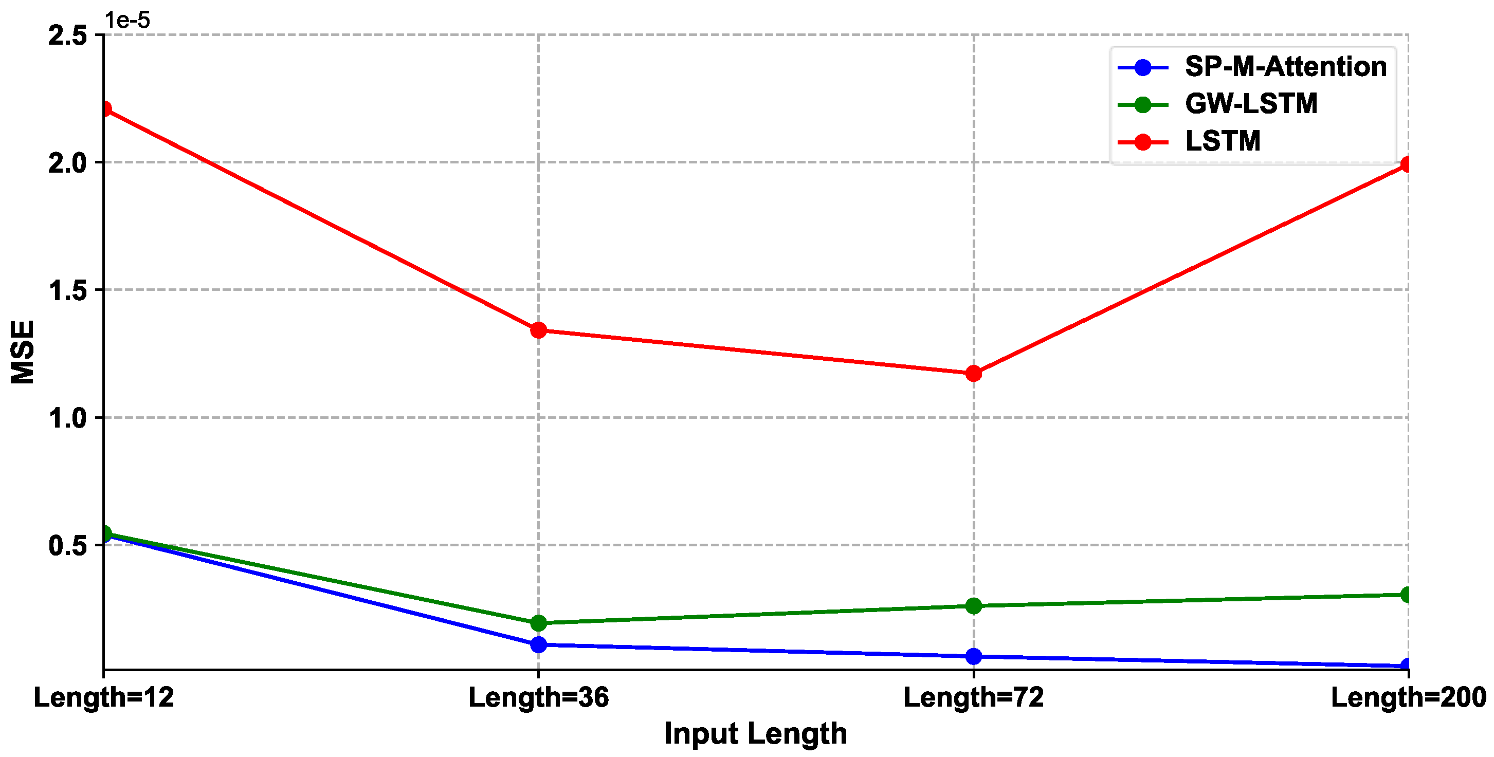
Looking at Table 3, we can see that all the evaluation functions of the proposed SP-M-Attention model are the smallest compared to other baseline models, which shows that the proposed model balances the short-term and long-term predictions very well and achieves the best performance overall with length distances. LSTM of the deep learning model is more effective than other machine learning and econometric methods, which shows that the deep learning model has a stronger ability of data feature fitting than traditional methods. We also observed that GW-LSTM, a hybrid model of recurrent neural networks and GARCH, surpasses other single models including LSTM to obtain the second prediction performance. Machine learning SVM and W-SVM are increasing in the input sequence, and the prediction accuracy is weakening, which shows that SVM has shortcomings in processing long sequences. EGARCH has a better prediction result than GARCH, which indicates that the financial volatility is asymmetric. With the increase in the length of the input sequence, the evaluation function of the GARCH method is stable and has no significant change, which reflects that the mathematical interpretation of this method is good, but the prediction accuracy is not ideal. When the length of the input reaches 100, the prediction performance of SVM is not improved and even deteriorates, which shows that the long-term memory ability of SVM is not significant. At the beginning of LSTM, as the length of input increases, the prediction accuracy increases slowly, and the acceleration decreases, which reflects that LSTM has some long-term memory ability, but the prediction effect is not obvious. With the increase in the length of the input sequence, the value of the prediction error function decreases at a steady speed, and the improvement of the prediction accuracy is obvious. Figure 7 shows the loss (MSE) trends of the SP-M-Attention, GW-LSTM, and LSTM models under different input lengths of SPX500.

The proposed method is a variant of the Transformer method and still belongs to the sequence-to-sequence structure in essence. Therefore, it has the ability of multi-step ahead prediction.

Table 4. Comparison errors (MSE) of multi-step ahead prediction between SP-M-Attention and other baseline methods.

Steps	SP-M-Attention	GW-LSTM	W-SVR	LSTM	SVR	HAR-RV	SV	EGARCH	GARCH
5	2.537 × 10−6	1.176 × 10−5	1.372 × 10−5	1.215 × 10−5	3.334 × 10−5	9.674 × 10−6	2.069 × 10−5	2.233 × 10−5	3.0174 × 10−5
10	2.824 × 10−6	1.294 × 10−5	1.509 × 10−5	1.336 × 10−5	3.668 × 10−5	1.064 × 10−5	2.276 × 10−5	2.457 × 10−5	3.087 × 10−5
20	3.152 × 10−6	1.424 × 10−5	1.660 × 10−5	1.470 × 10−5	4.035 × 10−5	1.171 × 10−5	2.504 × 10−5	2.703 × 10−5	3.396 × 10−5

lists the mean of multi-step ahead prediction errors(MSE) based on SP-M-Attention and other baseline methods on spx500. We obtain the information similar to the previous one-step ahead prediction, (a). The proposed method achieves the best prediction performance in all periods, which proves the effectiveness of the proposed method, (b). The MSE of all methods increases gradually with the increase in the step ahead, and the deterioration of SP-M-Attention is the slowest. This indicates that the proposed method has less error in multi-step ahead prediction of wave series. In the prediction of different forward steps, the relative improvement of the proposed model was over 5%. Overall, the results show that SP-M-Attention can accurately capture spatial and temporal correlations in related business sequences, which are of high predictive value.

Finally, we compared the predictive performance of different models under univariate and multivariate time series input conditions. In the case of the SPX500, volatility was entered into the model along with other variables (volume, the highest price, the lowest price, etc.) under the input condition of a multivariate time series. As shown in

Table 5. Comparison of MSE of SP-M-Attention with other baseline models for the multivariate volatility forecasting task.

	SP-M-Attention	GW-LSTM	W-SVR	LSTM	SVR	HAR-RV	SV	EGARCH	GARCH
MSE	2.340 × 10−7	1.801 × 10−6	1.172 × 10−5	1.090 × 10−5	2.557 × 10−5	8.256 × 10−6	1.612 × 10−5	1.891 × 10−5	2.610 × 10−5

, for the baseline deep learning model and our model, the average prediction error of multiple time series input conditions was smaller than that of the univariate input conditions. This phenomenon indicates that the deep learning model can learn the hidden correlation characteristics of multiple time series. SP-M-Attention achieves the best predictive accuracy overall baseline methods of multiple time series inputs.

To assess the statistical significance of these experimental results, we applied the Diebold–Mariano test to the comparisons between our proposed model and each of the baselines. As seen in

Table 6. The Diebold–Mariano (DM) test on volatility forecasting between SP-M-Attention and other baselines.

DM Test	BASELINES
	GW-LSTM	W-SVR	LSTM	SVR	HAR-RV	SV	EGARCH	GARCH
SP-M-Attention	−10.357 (0.00)	−16.819 (0.00)	−15.432 (0.00)	−33.762 (0.00)	−13.018 (0.00)	−20.664 (0.00)	−24.256 (0.00)	−35.246 (0.00)

The numbers outside the parentheses are statistics; p-values are inside the parentheses.

, the results of all Diebold–Mariano tests rejected the hypothesis that our model is insignificant compared to the baselines. Therefore, we can infer that our model has an advantage over all other models.

4.5. Discussions

In the previous section, we analyzed the prediction performance of the proposed model for low and medium frequency fluctuation series, such as the SPX500, WTI, and LGP index. The empirical results showed that the proposed model has an important advantage in predicting low-frequency data. Then, is the model proposed in this paper robust to emerging financial markets and high-frequency financial data? The robustness of a prediction method in finance is the key to its real practical application [35]. This section further uses the 5-min high-frequency data on the Shanghai Composite Index from January 2005 to December 2017 for modeling analysis to verify the robustness of the prediction model presented in this paper.

Table 7. Volatility prediction of different models on the high frequency of the Shanghai Composite Index.

	SP-M-Attention	GW-LSTM	W-SVR	LSTM	SVR	HAR-RV	SV	EGARCH	GARCH
MSE	3.153 × 10−8	2.592 × 10−7	1.715 × 10−6	1.615 × 10−6	3.692 × 10−6	1.196 × 10−6	2.331 × 10−6	2.742 × 10−6	3.850 × 10−6

shows the forecast metric (MSE) of different models outside the 5-min high-frequency data sample of the Shanghai Stock Exchange Composite Index.

From Table 7, we can see that each model’s forecast of high-frequency stock volatility was lower than the low-frequency data MSE, that is, had a smaller forecast error. At the same time, we found that the performance of SP-M-Attention was significantly improved by more than 10% compared to other baseline models in the volatility prediction task using high-frequency data from Asian stock markets. Our proposed model is still the best predictive model, and this conclusion is consistent with the conclusions of the previous section. This experiment confirms once again the value and robustness of our proposed method.

5. Conclusions

In this paper, we proposed a novel deep learning model, SP-M-Attention, for volatility prediction, which is a sparsely optimized, multi-headed, self-attentive neural network model. Because of the parallel processing mechanism of multi-headed attention, the proposed model has a larger perceptual field and captures complex features of volatility at different time scales and granularity more easily than classical time-series-like deep learning algorithms such as LSTM and GRU. Not only that, SP-M-Attention obtains the sparse representation of features using approximate sparse measurements, which greatly reduces the computational complexity of attention and the risk of gradient disappearance for long time series. Experiments on SPX500, WTI, and LGP showed that the proposed SP-M-Attention model has significant advantages and performs well in various types of financial volatility forecasting tasks. In addition, we analyzed the robustness of the proposed research methodology by using high-frequency data from emerging markets. The empirical results were consistent with the conclusions drawn from the low-frequency data. This fully demonstrates the robustness of the proposed model.

The SP-M-Attention model proposed in this paper is used to improve the accuracy of volatility forecasting. However, this does not mean that this approach can only solve this particular problem. It can also be extended to solve more time series problems with nonlinear and long-term memory characteristics, including complex forecasting problems in multiple domains such as traffic flow, energy consumption, disaster preparedness, and infectious disease prevention.

However, there are still limitations in our method that need further refinement. For example, (i) although we have found favorable evidence of the effectiveness of our method on several real datasets, the high-reward and high-risk nature of financial markets require a more in-depth and careful evaluation of the method before it can be applied in industry. We will continue our research work with the “paper trading” simulators. The proposed model is more effective and secure than others. In the absence of an actual capital commitment, these simulators can produce rolling forecasts of real-time data in the market through a rolling window, thus helping to correctly measure the value of the proposed model and further facilitating model optimization. Furthermore, (ii) in this paper, we only considered the joint modeling of volatility and other synchronous time variables. Still, many factors affect volatility, including non-synchronous time variables and even static variables and known future inputs. However, our current proposed model is not sufficient to solve such complex multi-span input forecasting problems. Therefore, volatility forecasting based on complex multi-span inputs will be the next step in our research. These are also directions for our continued research in the future.

References

- Engle, R.E. Autoregressive Conditional Heteroskedasticity with Estimates of the Variance of United Kingdom Inflation. Econometrica 1982, 50, 987–1007. [Google Scholar] [CrossRef]
- Bollerslev, T. Generalized autoregressive conditional heteroskedasticity. Econometrica 1986, 31, 307–327. [Google Scholar] [CrossRef] [Green Version]
- Brooks, C. A Double-threshold GARCH Model for the French Franc/Deutschmark exchange rate. J. Forecast. 2001, 20, 135–143. [Google Scholar] [CrossRef]
- Efimova, O.; Serletis, A. Energy markets volatility modelling using GARCH. Energy Econ. 2014, 43, 264–273. [Google Scholar] [CrossRef]
- Garcia, R.C.; Contreras, J.; Akkeren, M.V.; Garcia, J.B.C. A GARCH forecasting model to predict day-ahead electricity prices. IEEE Trans. Power Syst. 2005, 20, 867–874. [Google Scholar] [CrossRef]
- Kaiser, T. One-Factor-GARCH Models for German Stocks. Estim. Forecast. 1996, 30, 56–57. [Google Scholar]
- Klaassen, F. Improving GARCH volatility forecasts with regime-switching GARCH. Empir. Econ. 2002, 27, 363–394. [Google Scholar] [CrossRef] [Green Version]
- Abdalla, S.Z.S. Modelling Exchange Rate Volatility using GARCH Models: Empirical Evidence from Arab Countries. Int. J. Econ. Financ. 2012, 4, 216–229. [Google Scholar] [CrossRef]
- Agnolucci, P. Volatility in crude oil futures: A comparison of the predictive ability of GARCH and implied volatility models. Energy Econ. 2009, 31, 316–321. [Google Scholar] [CrossRef]
- Nelson, D.B. Conditional Heteroskedasticity in Asset Returns: A New Approach. Model. Stock Mark. Volatility 1991, 59, 347–370. [Google Scholar] [CrossRef]
- Melino, A.; Turnbull, S.M. Pricing foreign currency options with stochastic volatility. J. Econom. 1990, 45, 239–265. [Google Scholar] [CrossRef]
- Tse, Y.K. Stock returns volatility in the Tokyo stock exchange. Jpn. World Econ. 1991, 3, 285–298. [Google Scholar] [CrossRef]
- Mariani, M.C.; Bhuiyan, M.A.M.; Tweneboah, O.K.; Gonzalez-Huizar, H.; Florescu, I. Volatility models applied to geophysics and high frequency financial market data. Phys. A Stat. Mech. Appl. 2018, 503, 304–321. [Google Scholar] [CrossRef] [Green Version]
- Byun, S.-J.; Kim, S.; Rhee, D. Forecasting Future Volatility from Option Prices under the Stochastic Volatility Model. Ssrn Electron. J. 2009. [Google Scholar] [CrossRef]
- Andersen, T.G.; Benzoni, L. Realized Volatility. Ssrn Electron. J. 2008, 71, 555–575. [Google Scholar]
- Corsi, F.; Audrino, F.; Renò, R. HAR Modeling for Realized Volatility Forecasting; John Wiley & Sons, Inc.: New York, NY, USA, 2012. [Google Scholar]
- Qu, H.; Ji, P. Adaptive Heterogeneous Autoregressive Models of Realized Volatility Based on a Genetic Algorithm. Abstr. Appl. Anal. 2014, 2014, 943041. [Google Scholar] [CrossRef]
- Wei, Y. Forecasting volatility of fuel oil futures in China: GARCH-type, SV or realized volatility models? Phys. A Stat. Mech. Appl. 2012, 391, 5546–5556. [Google Scholar] [CrossRef]
- Gavrishchaka, V.V.; Banerjee, S. Support Vector Machine as an Efficient Framework for Stock Market Volatility Forecasting. Comput. Manag. Sci. 2006, 3, 147–160. [Google Scholar] [CrossRef]
- Bucci, A. Realized Volatility Forecasting with Neural Networks. J. Financ. Econom. 2019, 18, 502–531. [Google Scholar] [CrossRef]
- Hamid, S.A.; Iqbal, Z. Using neural networks for forecasting volatility of S&P 500 Index futures prices. J. Bus. Res. 2004, 57, 1116–1125. [Google Scholar]
- Tang, L.; Sheng, H.; Tang, L. Financial Prediction Based on Wavelet Support Vector Machine. Nat. Sci. J. Xiangtan Univ. 2009, 31, 58–63. [Google Scholar]
- Kristjanpoller, R.W.; Michell, V.K. A stock market risk forecasting model through integration of switching regime, ANFIS and GARCH techniques. Appl. Soft Comput. 2018, 67, 106–116. [Google Scholar] [CrossRef]
- Ramos-Pérez, E.; Alonso-González, P.J.; Núñez-Velázquez, J.J. Forecasting volatility with a stacked model based on a hybridized Artificial Neural Network. Expert Syst. Appl. 2019, 129, 1–9. [Google Scholar] [CrossRef]
- Fischer, T.; Krauss, C. Deep learning with long short-term memory networks for financial market predictions. Eur. J. Oper. Res. 2018, 270, 654–669. [Google Scholar] [CrossRef] [Green Version]
- Hochreiter, S.; Schmidhuber, J. Long Short-Term Memory. Neural Comput. 1997, 9, 1735–1780. [Google Scholar] [CrossRef] [PubMed]
- Kim, H.Y.; Won, C.H. Forecasting the Volatility of Stock Price Index: A Hybrid Model Integrating LSTM with Multiple GARCH-Type Models. Expert Syst. Appl. 2018, 103, 25–37. [Google Scholar] [CrossRef]
- Liu, Y. Novel volatility forecasting using deep learning–Long Short Term Memory Recurrent Neural Networks. Expert Syst. Appl. 2019, 132, 99–109. [Google Scholar] [CrossRef]
- Bahdanau, D.; Cho, K.; Bengio, Y. Neural Machine Translation by Jointly Learning to Align and Translate. arXiv 2014, arXiv:1409.0473v7. [Google Scholar]
- Cho, K.; Courville, A.; Bengio, Y. Describing Multimedia Content Using Attention-Based Encoder-Decoder Networks. IEEE Trans. Multimed. 2015, 17, 1875–1886. [Google Scholar] [CrossRef] [Green Version]
- Vaswani, A.; Shazeer, N.M.; Parmar, N.; Uszkoreit, J.; Jones, L.; Gomez, A.N.; Kaiser, L.; Polosukhin, I. Attention is All you Need. arXiv 2017, arXiv:abs/1706.03762. [Google Scholar]
- Zhou, H.; Zhang, S.; Peng, J.; Zhang, S.; Zhang, W. Informer: Beyond Efficient Transformer for Long Sequence Time-Series Forecasting. In Proceedings of the AAAI, Virtual Online, 2–9 February 2021. [Google Scholar]
- Álvarez-Díaz, M. Is it possible to accurately forecast the evolution of Brent crude oil prices? An answer based on parametric and nonparametric forecasting methods. Empir. Econ. 2020, 59, 1285–1305. [Google Scholar] [CrossRef]
- Lewis, M.; Liu, Y.; Goyal, N.; Ghazvininejad, M.; Zettlemoyer, L. BART: Denoising Sequence-to-Sequence Pre-training for Natural Language Generation, Translation, and Comprehension. arXiv 2019, arXiv:1910.13461. [Google Scholar]
- Gandhmal, D.P.; Kumar, K. Systematic analysis and review of stock market prediction techniques. Comput. Sci. Rev. 2019, 34, 100190. [Google Scholar] [CrossRef]
Figure 1.
Scaled dot-product attention.
Figure 2.
Computational flowchart of multi-head sparse self-attention.
Figure 3.
The architecture of SP-M-Attention.
Figure 4.
Residual learning block.
Figure 5.
Trends in the SPX500 Index (1950–2020).
Figure 6.
SPX500 Logarithmic return, historical volatility, and autocorrelation graphs.
Figure 7.
The LOSS (MSE) trends of SP-M-Attention, GW-LSTM, and LSTM models under different input lengths.