
On Training Knowledge Graph Embedding Models


1
Data Science Institute, National University of Ireland, H91 TK33 Galway, Ireland
2
Faculty of Informatics, Masaryk University, 602 00 Brno, Czech Republic
*
Author to whom correspondence should be addressed.
Information 2021, 12(4), 147; https://0-doi-org.brum.beds.ac.uk/10.3390/info12040147
Submission received: 8 February 2021
/
Revised: 17 March 2021
/
Accepted: 22 March 2021
/
Published: 31 March 2021
(This article belongs to the Collection Knowledge Graphs for Search and Recommendation)
Abstract
:Knowledge graph embedding (KGE) models have become popular means for making discoveries in knowledge graphs (e.g., RDF graphs) in an efficient and scalable manner. The key to success of these models is their ability to learn low-rank vector representations for knowledge graph entities and relations. Despite the rapid development of KGE models, state-of-the-art approaches have mostly focused on new ways to represent embeddings interaction functions (i.e., scoring functions). In this paper, we argue that the choice of other training components such as the loss function, hyperparameters and negative sampling strategies can also have substantial impact on the model efficiency. This area has been rather neglected by previous works so far and our contribution is towards closing this gap by a thorough analysis of possible choices of training loss functions, hyperparameters and negative sampling techniques. We finally investigate the effects of specific choices on the scalability and accuracy of knowledge graph embedding models.
1. Introduction
The recent advent of knowledge graph embedding (KGE) models has allowed for scalable and efficient manipulation of large knowledge graphs (KGs) such as RDF Graphs, improving the results of a wide range of tasks such as link prediction [1,2,3], entity resolution [4,5] and entity classification [6]. KGE models operate by learning embeddings in a low-dimensional continuous space from the relational information contained in the KG while preserving its inherent structure. Specifically, their objective is to rank knowledge facts—relational triples connecting subject and object entities s and o by a relation type p—based on their relevance. Various interactions between their entity and relation embeddings are used for computing the knowledge fact ranking. These interactions are typically reflected in a model-specific scoring function.
For instance, TransE [1] uses a scoring function defined as the distance between the o embedding and the translation of the embedding associated with s by the relation type p embedding. DistMult [7], ComplEx [8] and HolE [9] use multiplicative composition of the entity embeddings and the relation type embeddings. This leads to a better reflection of the relational semantics and leads to state-of-the-art performance results (refer to [10] for a review). Although there is a growing body of literature proposing different KG models (mostly focusing on the design of new scoring functions), other parts of the knowledge graph embedding learning process, e.g., loss functions, and negative sampling strategies have not received much attention to date [11].
This has already been shown to influence the behaviour of the KGE models. For instance, Ref. [12] observed that, despite the different motivations behind HolE and CompleEx models, they have equivalent scoring functions. However, their performance still differs. Trouillon et al. [13] have concluded that this difference is caused by the fact that HolE uses a max-margin loss while ComplEx a log-likelihood loss. This shows that cost functions are important for thorough understanding, and even improvement of the performance of different KGE models.
Other than loss function selection, the studies of Dettmers et al. [14] and Lacroix et al. [15] have shown that using 1-vs.-all negative sampling strategy can significantly enhance the accuracy of KGE models. Furthermore, Kadlec et al. [16] have also shown that the accuracy of KGE models is sensitive to the training parameters where minor changes to the parameters can significantly change the output models’ accuracy. Despite the importance of all the previously mentioned parts of the KGE learning process, a comprehensive study is still missing. This study is a step towards improving our understanding of the influence of the different parts of the training pipeline on the behaviour of KGE models. Our analysis specifically focuses on investigating the effects of training parts on both the scalability and accuracy of KGE models. We first investigate KGE loss functions and their different approaches, and we assess the effects of the loss function choice on different KGE models. We then study KGE negative sampling strategies and effects on both accuracy and scalability. We finally discuss the effects of training parameters such as the embedding size, batch size, among others, on the scalability and accuracy of different KGE models.
Despite the growing number of KGE models and their different new approaches, we limit our study to a basic set of models: the TransE [1], DistMult [7], TriModel [17], CP [18], and Complex [8] models which represent the most popular and publicly available methods. We use these methods as simple examples to examine and showcase the different parts of the KGE learning process, where each of these model act as a representative of a unique class of knowledge graph embedding models. For example, the TransE model is distance-based model which update the knowledge graph embeddings based on the distance between the entities in the vector space. On the other hand, the DistMult and ComplEx models are factorization based models which operate using a matrix factorization procedure, the complex model, however, belong to the class of the multi-vector embedding models where it represents each entity and relation in the graph using two embedding vectors.
The summary of our contributions is as follows:
- We provide a comprehensive analysis of training loss functions as used in several state-of-the-art KGE models in Section 3. We also preform an empirical evaluation of different KGE models with different loss functions and we show the effect of these losses on the KGE models predictive accuracy.
- We study negative sampling strategies and we examine their effects on the accuracy and scalability of KGE models.
- We study the effects of changes in the different hyperparameters and their effects on the accuracy and scalability of KGE models during the training process.
2. Background
In this section, we discuss the concepts and notation used throughout the study. We discuss knowledge graph embedding models, learn to rank training objectives and the different metrics for evaluating knowledge graph embedding models in the task of link prediction.
We use the following notation in the rest of the paper. Let be a set of objects (triples) to be ranked. Let be a labelling function where is the label of object x (e.g., true/false or an arbitrary integer in case of multi-label problems). By default, we assume a binary labelling for triples, , where 0 and 1 represent false and true labels, respectively.
Let be the set of possible scoring functions. Given a KGE model, is its scoring function, where f aims to score triples in X such that positive triples are scored higher than negative ones, formally, . Finally, denotes the rank position of element according to scoring function f, or the position of score in a descending order of all scores for all .
2.1. Loss Functions in Learning to Rank
In learning to rank, models typically use loss functions to learn the optimal scoring function parameters from training data. The learning process then involves minimising a loss function defined on the basis of the objects, their labels, and the scoring function. In learning to rank models, the objective is to score a set of labelled objects such that: for each two objects with different label values, the object with greater label value also has greater model score. Next, we present the several approaches proposed in learning to rank to learn optimal scoring functions.
- Pairwise approach. The loss is defined as the summation of the differences between the predicted score of an element and the scores of other elements with a smaller labels’ value. The formula is as follows:where the function can be the hinge function as in Translating Embeddings model [1] or the exponential function as in RankBoost [20].
- Listwise approach. The loss is defined as a comparison between the rank permutation probabilities of model scores and values of actual labels [21]. Let be an increasing and strictly positive function. We define the probability of an object being ranked on the top (a.k.a. top one probability), given the scores of all the objects as:where is the score of object i, . The listwise loss can then be defined as:where is a model-dependent loss and is a labelling function which returns the true label of x. Possible examples include cross-entropy in ListNet [21] or likelihood loss as in ListMLE [22].
2.2. Knowledge Graph Embedding Process
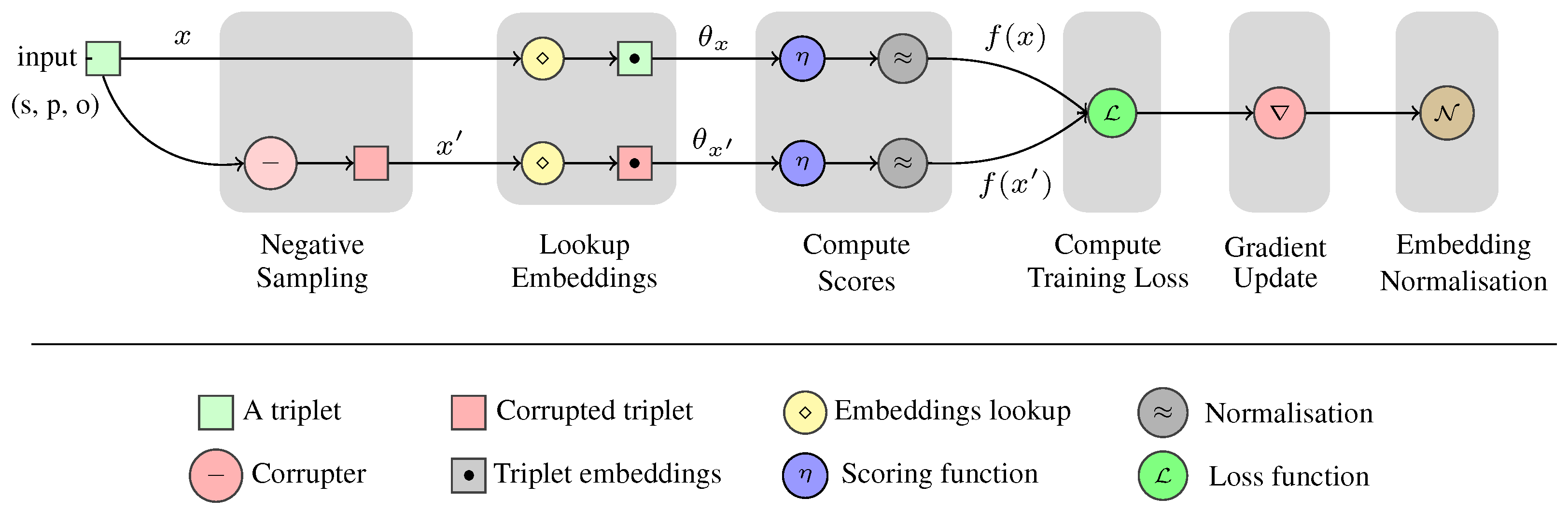
Knowledge graph embedding models learn low rank vector representation i.e., embeddings for graph entities and relations. In the link prediction task, they learn embeddings in order to rank knowledge graph facts according to their factuality. The process of learning these embeddings consists of different phases as shown in Figure 1. First, they initialise the embeddings of both relations and entities using random noise. These embeddings are then used to score a set of true and false facts, where the scores of facts are generated by computing the interaction between their subject, predicate and object embeddings using a model dependent scoring function. Finally, embeddings are updated through a gradient descent routine which minimises a training loss that usually represents a min-max loss over the scored facts. The objective is then to maximise the scores of true facts and minimise the scores of other facts.
2.2.1. Negative Sampling
In learning to rank approaches, models use a ranking loss, e.g., pointwise or pairwise loss, to rank a set of true and negative instances [23], where negative instances are generated by corrupting true training facts with a given ratio of negative to positive instances [1]. This corruption happens by changing either the subject or object of the true triple instance. In this configuration, the ratio of negative to positive instances is traditionally learnt using a grid search, where models compromise between the accuracy achieved by increasing the ratio and the runtime required for training.
On the other hand, multi-class based models train to rank positive triples against all their possible corruptions as a multi-class problem, where the range of classes is the set of all entities. For example, training on a triple is achieved by learning the right classes “s” and “o” for the pairs and , respectively, where the set of possible classes is E of size . Despite the enhancement of predictions’ accuracy achieved by such approaches [14,15], their negative sampling procedure is exhaustive and requires a high space complexity due to the usage of the whole entity vocabulary per each triple.
2.2.2. Embedding Interactions
After KGE models produce negative samples from input triples, they generate scores for both the true and negative (corrupted) triples. These scores are generated using embedding interaction function, i.e., scoring functions. First, the model looks up the embeddings of the subject, predicate and object of triples. Then, the model uses an embedding interaction function to learn a score for each triple using its embeddings.
The embedding interaction functions are model-dependent and they operate using different approaches such as embedding translation [1], linear products [7] and convolutional filters [14]. For example, the TransE model uses a translation-based scoring function which encodes embedding interactions as a translation from the subject embedding vector to the object embedding vector through the predicate vector [1]. Such an approach allowed highly scalable knowledge graph embedding with linear time and space complexity. However, it suffered from limited ability to encode 1-to-many predicates in knowledge graphs due to dependence on direct additive translations [7]. Later models such as DistMult used a linear product-based scoring functions which allowed better encoding of 1-to-many predicates while preserving the linear time and space complexity. However, DistMult model’s scoring function suffered of limited ability to preserve the predicate direction due to a dependence on a symmetric operation [7].
More recent approaches, such as ComplEx [8], ConvE [14], TriModel [17], among others, propose new scoring mechanisms which allow for encoding both 1-to-many relations and preserve the predicate directionality within linear time and space complexity. Since these scoring functions are well covered in previous studies, we will not discuss the details of their mechanisms-of-action in our study. For further information and technical details about these knowledge graph embedding scoring functions, we refer the readers to the reviews of Nickel et al. [9] and Wang et al. [10].
In the following, we provide a further discussion and definition of the embedding interaction functions of the models that we examine in our study, where we discuss them within their embedding strategy.
- Distance-based embeddings’ interactions
The Translating Embedding model (TransE) [1] is one of the early models that use distance between embeddings to generate triple scores. It interprets triple’s embeddings interactions as a linear translation of the subject to the object such that , and generates a score for a triple as follows:
where true facts have zero score and false facts have higher scores. This approach provides scalable and efficient embeddings learning as it has linear time and space complexity. However, it fails to provide efficient representation for interactions in one-to-many, many-to-many and many-to-one predicates as its design assumes one object per each subject–predicate combination:
- Factorisation-based embedding interactions
Interactions based on embedding factorisation provide better representation for predicates with high cardinality. They have been adopted in models like DistMult [24] and ComplEx [8]. The DistMult model uses the bilinear product of embeddings of the subject, the predicate, and the object as their interaction, and its scoring function is defined as follows:
where is the k-th component of subject entity s embedding vector . DistMult achieved a significant improvement in accuracy in the task of link prediction over models like TransE. However, the symmetry of embedding scoring functions affects its predictive power on asymmetric predicates as it cannot capture the direction of the predicate. On the other hand, the ComplEx model uses embedding in a complex form to model data with asymmetry. It models embeddings interactions using the the product of complex embeddings, and its scores are defined as follows:
where represents the real part of complex number x and all embeddings are in complex form such that , and are respectively the real and imaginary parts of e, and is the complex conjugate of the object embeddings such that and this introduces asymmetry to the scoring function. Using this notation, ComplEx can handle data with asymmetric predicates and keep scores in the real spaces; it only uses the real part of embeddings’ product outcome. ComplEx preserves both linear time and linear space complexities as in TransE and DistMult; however, it surpasses their accuracy in the task of link prediction due to its ability to model a wider set of predicate types.
2.3. Ranking Evaluation Metrics
Learning to rank models are evaluated using different ranking measures including Mean Average Precision (MAP), Normalised Discounted Cumulative Gain (NDCG), and Mean Reciprocal Rank (MRR) [25]. Below, we discuss MAP and MRR based on a set of queries . (Note that our experiments will also use Hits@k metric for the model comparison; our proposed cost function design is independent of that metric and therefore we do not provide detailed definitions here.)
- Mean Average Precision (MAP). MAP is a ranking measure that evaluates the quality of a rank depending on the whole rank of its true (relevant) elements. First, we need to define Precision at position k (denoted as ):where and is an indicator function that is equal to 1 when x is a relevant element and 0 otherwise.The Average Precision (AP) is defined by:where n is the total number of objects associated with query q, and is the number of objects with label one. The MAP is then defined as the mean of AP over all queries Q:
- Mean Reciprocal Rank (MRR). The Reciprocal Rank (RR) is a statistical measure used to evaluate the response of ranking models depending on the rank of the first correct answer. The MRR is the average of the reciprocal ranks of results for different queries in Q. Formally, MRR is defined as:where is the highest ranked relevant item for query . Values of RR and MRR have a maximum of 1 for queries with true items ranked first, and get closer to 0 when the first true item is ranked in lower positions. Therefore, we can define the MRR error as . This error starts from 0 when the first true item is ranked first, and increases towards 1 for less successful rankings.
- Hits@k. This metric represents the number of correct elements predicted among the top-k elements in a rank, where we use Hits@1, Hits@3 and Hits@10. This metric indicates that the model’s probability of ranking a relevant (true) fact in the top-k element scores in the rank.
2.4. Experimental Evaluation
For this study, we have selected three highly studied models in the state of the art and selected five commonly used datasets for link prediction. Our goal here is to learn knowledge graph embeddings for each dataset applying different losses and analysing their performance. We describe the setup of our experiments using the TransE [1], DistMult [7], and ComplEx [8] KGE models. Then, we present the characteristics of the benchmarking datasets, and also provide the relevant implementation details.
Table 1 contains statistics of the five benchmarking datasets used in our experiments (All the benchmarking datasets can be downloaded using the following URL: https://0-doi-org.brum.beds.ac.uk/10.6084/m9.figshare.14213894, accessed on 20 March 2021). Three of them, namely, WN18RR, FB15k-237, and YAGO10 are among the most frequently used datasets for benchmarking KGE models. In addition, here we consider the NELL239 and PSE, which contain a higher number of entities and triples for studying the scalability of KGE models.
- ●
- Benchmarking Datasets. In our experiments, we use five knowledge graph benchmarking datasets:
- PSE: a poly-pharmacy side-effects dataset [33] containing facts about drug combinations and their related side-effects. The dataset was introduced by Zitnik et al. [33] to study modelling poly-pharmacy side-effects using knowledge graph embedding models. Since the dataset is significantly larger than the available standard benchmark we use it to study the effects of hyperparameters and accuracy of the knowledge graph embedding models.
- ●
- Evaluation Protocol. We evaluate the KGE models using a unified protocol that assesses their performance in the task of link prediction. Let X be the set of facts, i.e., triples; be the embeddings of entities E, and be the embeddings of relations R. The KGE evaluation protocol works in three steps:
- (1)
- Corruption: For each , x is corrupted times by replacing its subject and object entities with all the other entities in E. The corrupted triples can be defined as:where and . These corruptions effectively provide negative examples for the supervised training and testing process due to the Local Closed World Assumption [34], frequently adopted for knowledge graph mining tasks.
- (2)
- Scoring: Both original triples and corrupted instances are evaluated using a model-dependent scoring function. This process involves looking up embeddings of entities and relations, and computing scores depending on these embeddings.
- (3)
- Evaluation: Each triple and its corresponding corruption triples are evaluated using the RR ranking metric as a separate query, where the original triples represent true objects and their corruptions false ones. It is possible that corruptions of triples may contain positive instances that exist among training or validation triples. In our experiments, we alleviate this problem by filtering out positive instances in the triple corruptions. Therefore, MRR and Hits@k are computed using the knowledge graph original triples and non-positive corruptions only [1].
3. Loss Functions in KGE Models
Generally, KGE models are cast as learning to rank problems. They employ multiple training loss functions that comply with the ranking loss approaches. In the state-of-the-art KGE models, loss functions have been designed according to various pointwise and pairwise approaches that we review next.
3.1. KGE Pointwise Losses
First, we discuss current pointwise loss functions for KGE models including SE, hinge, and logistic losses. We then propose a new pointwise loss function, namely, the Pointwise Square Loss (PSL) that combines the square growth of SE and the configurable margin of hinge loss.
- Pointwise square error loss (SE). It is a pointwise ranking loss function used in RESCAL [4]. It models training losses with the objective of minimising the squared difference between model predicted scores for triples and their true labels:The optimal score for true and false facts is 1 and 0, respectively. A nice to have characteristic of the SE loss is that it does not require configurable training parameters, shrinking the search space of hyperparameters compared to other losses (e.g., the margin parameter of the hinge loss).
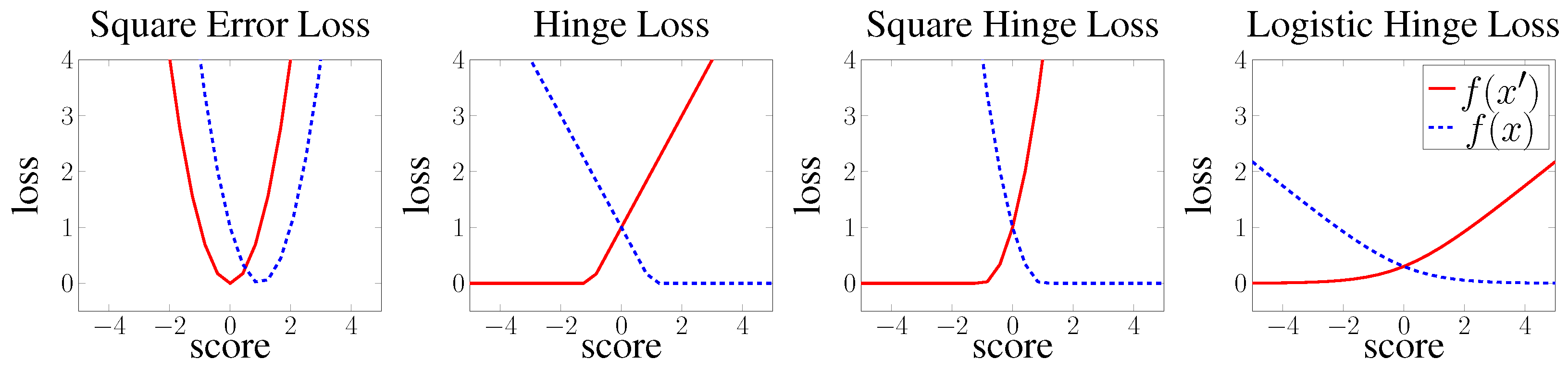
- Pointwise hinge loss. Hinge loss can be interpreted as a pointwise loss, where the objective is to generally minimise the scores of negative facts and maximise the scores of positive facts to a specific configurable value. This approach is used in HolE [9], and it is defined as:where is an abbreviation for pointwise to clarify the type of the loss, if x is true and otherwise, and denotes the function. This effectively generates two different loss slopes for positive and negative scores as shown in Figure 2. Thus, the objective resembles a pointwise loss that minimises negative scores to reach , and maximises positives scores to reach .
- Pointwise logistic loss. The ComplEx [8] model uses a logistic loss, which is a smoother version of pointwise hinge loss without the configurable margin parameter. Logistic loss uses a logistic function to minimise the negative triples score and maximise the positive triples score. This is similar to hinge loss, but uses a smoother linear loss slope defined as:where is the true label of fact x, which is equal to 1 for positive facts and equal to otherwise.
3.2. KGE Pairwise Losses
Here, we discuss established pairwise loss functions in KGE model which are summarised in Figure 3.
- Pairwise hinge loss. Hinge loss is a linear learning to rank loss that can be implemented in both a pointwise or pairwise loss settings. In both, the TransE [1] and DistMult [7] models the hinge loss is used in its pairwise form and defined as follows:where the term is an abbreviation for pairwise, is the set of true facts, is the set of false facts, and is a configurable margin that separates positive from negative facts.
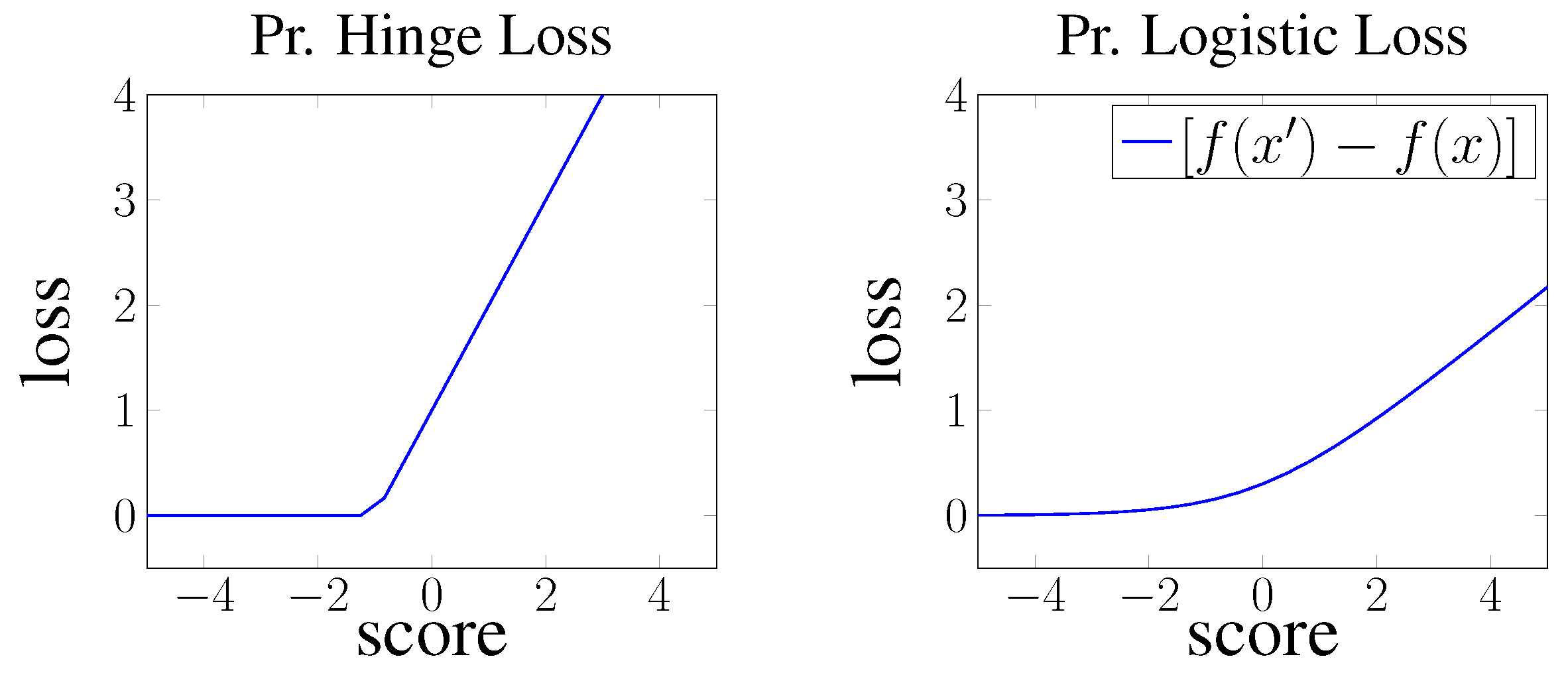
In this case, the objective is to minimise the marginal difference (difference of scores with the added margin) between the scores of negative and positive instances. This approach optimises towards having embeddings that satisfy as shown in Figure 3.
- Pairwise logistic loss. Logistic loss can also be interpreted as pairwise margin based loss following the same approach as in hinge loss. The loss is then defined as:where the objective is to minimise the marginal difference between negative and positive scores with a smoother linear slope than hinge loss as shown in Figure 3.
3.3. KGE Multi-Class Losses
In the following, we discuss KGE loss functions that are used to cast the KGE process into a multi-class classification problem.
- Binary cross entropy loss (BCE). The authors of the ConvE model [14] proposed a new binary cross entropy multi-class loss to model the training error of KGE models in link prediction. In this setting, the whole vocabulary of entities is used to train each positive fact such that for a triple , all facts with and are considered false. The BCE loss can be defined as follows:where is the true label of triplet . Despite the extra computational cost of this approach, it allowed ConvE to generalise over a larger sample of negative instances, therefore surpassing other approaches in accuracy [14].
- Negative-log softmax loss (NLS). In a recent work, Lacroix et al. [15] introduced a soft-max regression loss to model training error of the ComplEx model as a multi-class problem. In this approach, the objective for each triple is to minimise the following loss:where is the model score for the triple , and , , and . This resembles a log-loss of the soft-max value of the positive triple compared to all possible object and subject corruptions where the objective is to maximise positive fact scores and minimise all other scores. This approach achieved significant improvement to the prediction accuracy of ComplEx model over all benchmark datasets when used with the 3-nuclear norm regularisation of embeddings [15].
3.4. Effects of Training Objectives on Accuracy
We performed an experimental evaluation for the effect of loss function on the accuracy of KGE models in the link prediction task in terms of MRR and Hits@10. For simplicity, we have only experimented with three KGE models: TransE, DistMult and ComplEx. These models are used as examples where we assess their performance on different benchmarks under different loss function configurations.
Table 2 summarises the outcome of our experiments, comparing the accuracy of the models on both ranking and multi-class loss approaches in terms of MRR and Hits@10. Interestingly, in the context of the ranking loss configuration, we can observe that the default loss functions of the examined models do not always yield the best results. On the contrary, The DistMult and ComplEx models which by default use the pointwise hinge and logistic losses, respectively, obtain their best result using the pointwise square error loss with all the examined benchmarks. This shows that changing the default loss function of these models can help enhance their predictive accuracy. The results of the TransE model also show that its default loss configuration achieves the best results on 4 out of 6 examined evaluation metrics. On the other hand, the pairwise logistic loss configuration of TransE achieves best results in 3 out of 6 of the examined evaluation metrics. Given that the pairwise logistic loss does not require parameters—unlike the margin-based hinge loss—the pairwise logistic loss can be a preferred configuration for TransE as it can significantly reduce the grid search time.
Our results also show that the multi-class loss versions of the CP, DistMult, ComplEx models have significantly better results than their ranking based losses. For example, on the NELL239 dataset, the best performing ranking-based approach, the complex model with the pointwise square error loss, achieves 0.35 and 0.52 scores in terms of MRR and Hits@10, respectively, compared to its NLS loss version which achieves 0.40 and 0.58 scores, respectively. The results also show that the best multi-class loss results are obtained using the negative log soft-max loss. It is noteworthy that both multi-class based versions of the DistMult and ComplEx achieve their best results using the negative soft-max loss.
3.5. Effects of Training Objectives on Scalability
We have shown that different training objectives yield significantly different results for the same KGE models. Our experimental results also suggested that the multi-class loss functions achieve the best results in terms of MRR and Hits@10 on all the investigated datasets. However, this approach uses a 1-vs.-all negative sampling strategy which is time-consuming due to its higher time and space complexity compared to usual 1-vs.-n sampling. In the following, we compare the ranking losses and multi-class losses in terms of the runtime required for training a KGE on different dataset size to study the scalability of both approaches.
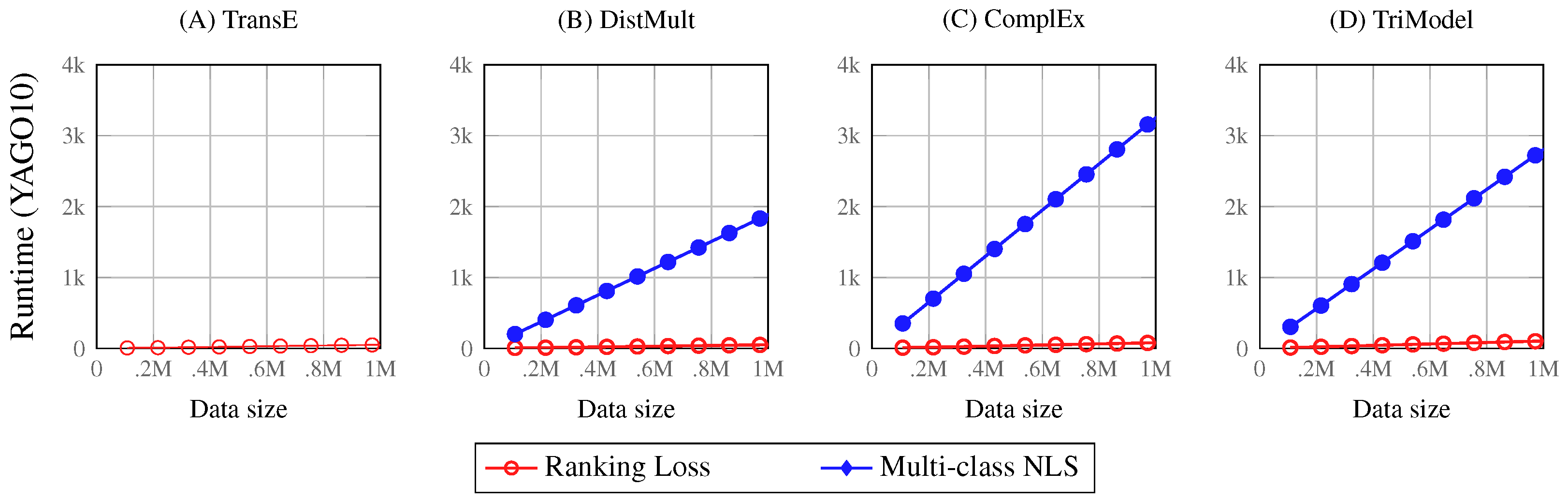
We execute an experiment using the YAGO10 benchmark, where we train KGE models on different percentages of the dataset and study the relation between the growth of the dataset size and the required training runtime. Moreover, we compare the training runtime of different KGE models with the negative soft-max loss (NLS) and the pointwise square error loss as representatives of their respective loss class.
Figure 4 shows the outcomes of our experiments, presenting a series of plots which describe the relation between the growth of the dataset size and the growth of training runtime of both ranking and multi-class loss approaches. As expected, the results show that the multi-class losses have significantly higher training runtime than ranking losses for all the KGE models. The runtime of the ranking loss functions appears to be constant; however, it is growing with a constant increase related to the growth of the training data. On the other hand, the multi-class loss functions have a linear growth which correlates to the growth of the training data. This shows the significant difference between both training loss approaches in terms of the scalability of the training process.
The results also show that the multi-class losses have different growth slopes than the DistMult, ComplEx and TriModel approaches. These different results from their different techniques in modelling embedding interactions that have a significant effect on the training time with 1-vs.-all negative sampling (multi-class losses). The different slopes corresponding to the DistMult, ComplEx and TriModel are a result of the different number of embedding vectors they use. While the DistMult model uses one embedding vector, the ComplEx model uses two and the TriModel uses three, which affects their scalability.
4. KGE Training Hyperparameters
In this section, we discuss the effects of training hyperparameters on both the accuracy and scalability of knowledge graph embedding models. We first discuss the effects in terms of scalability and we then discuss the implications of changes of hyperparameters on the accuracy of KGE models in the task of link prediction.
4.1. Training Hyperparameters Effects on KGE Scalability
Knowledge graph embedding models are famous for their high quality predictions with high scalability [34]. Most of the KGE methods employ linear transformations such as vector translations and vector diagonal products to learn interactions between embeddings, therefore, they operate within linear time and space complexity [8,15,17].
Despite the high scalability of the training process KGE models, they require the hyperparameters’ training routine which is time consuming due to the large hyperparameters’ search space. Traditionally, the hyperparameters search is executed using grid search to find the best hyperparameters for each model on each new dataset. The training hyperparameters of KGE models include embedding size, negative samples per positive, batch size, etc. Kadlec et al. [16] have shown that minor changes to these hyperparameters can yield significantly different results in terms of the models’ resulting accuracy. The changes in these hyperparameters also have an impact on their runtime where changes in hyperparameters such as the embedding size and the number of sampled negatives can affect the memory space used during training.
We performed an experimental evaluation for four different KGE models: TransE, DistMult, Complex and TriModel, where we examine the effects of changes of the training hyperparameters and data size on their training runtime. We use the PSE benchmarking dataset [33]—our largest benchmarking dataset—to show the effect of hyperparameters on training runtimes of KGE models.
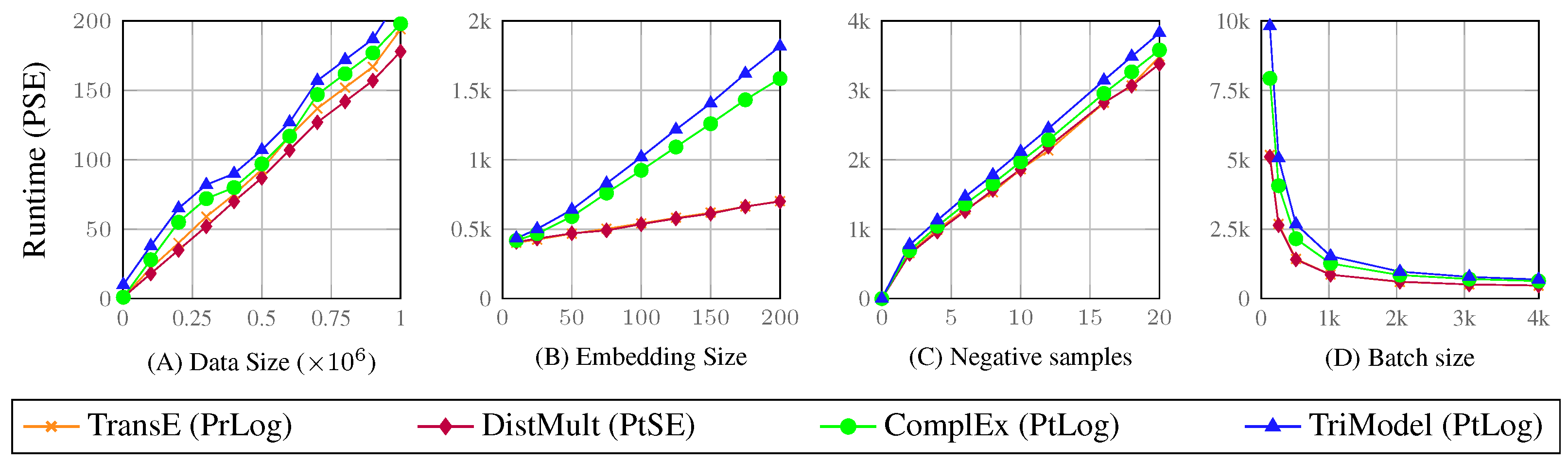
Figure 5 shows the outcome results of our experiments across the different investigated training hyperparameters. In these experiments, we use a set of fixed hyperparameters (embedding size = 150, batch size = 2048, negative samples = 2, training iterations = 500) and we use a set of values for each of the investigated hyperparameter in their respective experiment to show the relation between the changes of the hyperparameters and the KGE model’s accuracy and runtime. The plot “A” shows the relation between the training runtime and the size of the processed data. The plot shows that all the four investigated models have a linear relation between their training runtime and the data size. We can also observe that the models have a consistent growth in terms of their runtime across all the data sizes. The DistMult model consistency achieves the smallest runtime followed by the TransE, TriModel and ComplEx models.
Plot “B” shows the relationship between the training runtime and the model embedding size. The plot shows that all the investigated models have a linear growth of their training runtime corresponding to the growth of the embeddings size. However, the growth rate of the TransE and DistMult models is considerably smaller than the growth of both the ComplEx and TriModel models. This occurs as both the TransE and DistMult models use a single vector to represent each of their embeddings while the ComplEx and TriModel models use two and three vectors, respectively. Despite the better scalability of both the TransE and DistMult models, the ComplEx and TriModel models generally achieve better predictive accuracy [17].
The plot “C” shows the relation between the runtime of KGE models and the number of negative samples they use during training. The plot shows that there is a positive linear relation between training runtime and the number of negative samples—where all the KGE models have similar results across all the investigated sampling sizes. The TriModel, however, consistently have the highest runtime compared to other models.
Plot “D” shows the effects of the size of the batch on the training runtime. The plot shows an exponential decay of the training runtime with the linear growth of the data batch size. The KGE models process all the training data for each training iteration (i.e., epoch), where the data are divided into batches for scalability and generalisation purposes. Therefore, the increase of the training data batch sizes leads to a decrease of the number of model executions for each training iteration. Despite the high scalability that can be achieved with large batch sizes, the best predictive accuracy is often achieved using small data batch sizes. Usually, the most efficient training data batch size is chosen during a hyperparameter grid search along with other hyperparameters such as the embedding size and the number of negative samples.
The runtime of the models reported in Figure 5 looks very similar or almost identical for all the models as they all operate using the same training procedure, where they differ only on the way they represent the embeddings and compute their interactions. This is significantly shown in the plot (B) in Figure 5, which shows a significant difference in terms of runtime between models that use single embedding vectors such as TransE and DistMult and other models which use multi-vector embeddings such as ComplEx and TriModel.
The reported predictive accuracy of the models in terms of the MRR scores in Figure 6 looks similar as the models parameters were not properly tuned. The reported models are also known to produce very similar or almost identical results on the WN18RR benchmark [17]. The purpose of the figure is also to study the change of the models predictive accuracy in relation to the change of the values of the models’ hyperparameters and not the best possible model accuracy.
Analysis of the Predictive Scalability Experiments
Our experiments on the effects of training parameters of KGE models on the models’ scalability suggest the following:
- The results confirm that KGE models have linear time complexity as shown in Figure 5 where the models’ runtime grows linearly corresponding to increase of both data size and embedding vector sizes.
- The results also confirm that models such as the TriModel and Complex model which have more than one embedding vector for each entity, and relations require more training time compared to models with only one embedding vector.
- The results also show that the training batch size has a significant effect on the training runtime, therefore, using larger batch sizes are suggested to significantly decrease the training runtime of the training of KGE models.
4.2. Training Hyperparameters’ Effects on KGE Accuracy
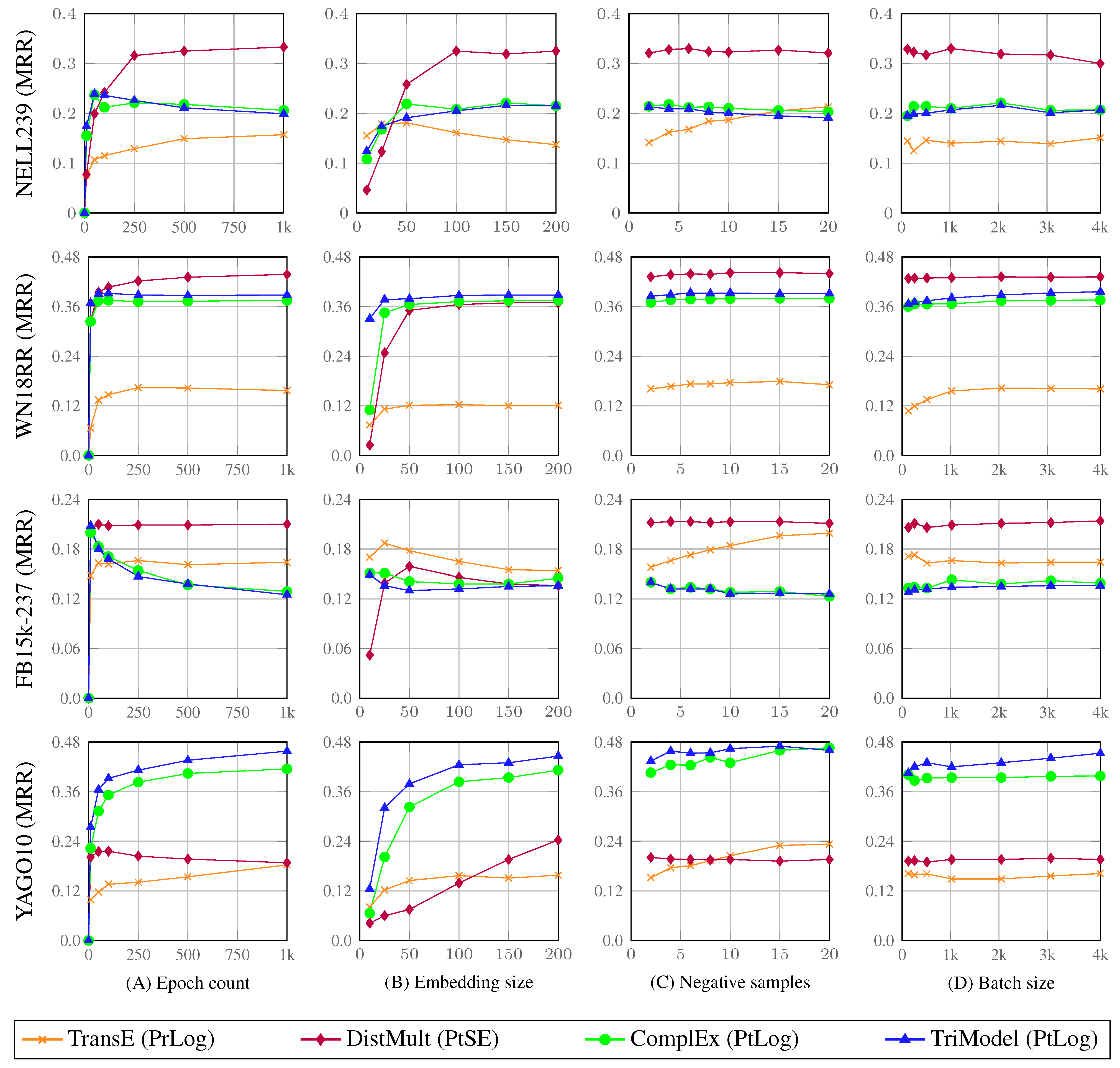
In the following, we study the relation between changes in different training hyperparameters and the accuracy of KGE models. We perform an experimental evaluation where we examine the changes of the accuracy of KGE models in terms of MRR compared to the changes of the model’s training hyperparameters. Figure 6 shows the outcome of our experiments where the plots present the changes on MRR corresponding to changes of the training hyperparameters of different KGE models on the NELL239, WN18RR, FB15k-237 and YAGO10 datasets.
The datasets reported in Figure 6 are sorted in a descending order from top to down in terms of the number of facts contained in the dataset (dataset size). The first row of plots corresponds to the experiments which are done on the NELL239 dataset (the smallest dataset); these results show that changing the number of training iteration (epochs) and the embedding size has a significant effect on models’ accuracy. On the other hand, the negative samples and batch size hyperparameters have less effect on the models’ MRR score where the change in the batch size and the number of negative samples insignificantly affects the MRR score—except by the TransE model which has a positive MRR score relation with the number of negative samples.
The results corresponding to the WN18RR dataset also show that the epoch count and embedding size have a significant effect of the model’s accuracy. We can also observe that both hyperparameters have a positive relation with the MRR score of KGE models compared to the variable relation on the NELL dataset. The results also show that the MRR score of KGE models stabilises after 250 training iterations with an embedding size of 50—increases above these values do not have significant effects on the MRR score of models. Similar to the results on the NELL239, the negative samples and batch size hyperparameters show no significant relation with the MRR scores of different KGE models.
The results of the FB15k-237 dataset have a different relation pattern corresponding to the number of training iterations compared to other datasets where the MRR scores of different KGE models have negative or no relation with the changes of the number of training iterations. For example, the MRR scores TransE and DistMult approximately have the sample values corresponding to all the different values of the number of training iterations. On the other hand, the TriModel and ComplEx models have a negative relation with the number of training iteration where their MRR scores decrease with the growth of the training iterations count. The changes of the embedding size on KGE models on the FB15k-237 dataset also show variant patterns where different KGE models have different relation to the change of the size of the embeddings.
On the other hand, the changes of the batch size and number of negative samples follow a similar pattern as in the NELL239 dataset: the models’ MRR scores have no significant relation with the changes of both hyperparameters. However, an exception was observed for the TransE model, which has a positive MRR score relation with the number of negative samples.
The results of the YAGO10 dataset (the largest dataset in this experiment) show a positive relation between the number of training iterations and the MRR score of the TransE, TriModel and ComplEx models. Conversely, the DistMult model has a negative relation with the the number of training iterations. These results show that all models have a positive relation between their MRR scores and the size of the embeddings. For the batch size and negative samples’ hyperparameters, we can observe that there is a lower correlation to the MRR scores as in the previous dataset; however, there is a noticeable low positive correlation between the number of negative samples and the MRR scores of the TransE, TriModel and ComplEx models.
Finally, based on the observations previously presented, we can provide a list of practical suggestions for anyone experimenting with KGE models:
- Changes on the embedding vectors’ size have the biggest effect on the predictive accuracy of KGE models. Thus, we suggest to carefully select this parameter by searching through a larger search space, which can help with ensuring that the models can reach their best representations of the knowledge graph.
- The increased number of training iterations can sometimes have a negative effect on the outcome predictive accuracy. Thus, we suggest using early stopping techniques to decide when to stop model training before accuracy starts to decrease.
- Both the number of negative samples and batch sizes showed a small effect on the predictive accuracy of KGE models. Thus, this parameter can either be assigned fixed values or be found using a small search spaces to help decrease the hyperparameters search space, and thus the hyperparameters’ tuning runtime.
5. Discussion
In this section, we discuss the compromise between scalability and accuracy in the training of KGE models. We also discuss the properties of some datasets and their relation with KGE interaction functions. We finally discuss the compatibility between specific KGE scoring and loss functions.
5.1. The Compromise between Scalability and Accuracy
We have shown that KGE models achieve their best result in terms of accuracy using multi-class loss functions. However, these functions depend on the 1-vs.-all negative sampling which is time-consuming as we have shown in Section 3.5. On the other hand, KGE models with ranking-based loss function are significantly more scalable, but they have less accurate predictions compared to the multi-class losses. This variability between the capabilities of the two approaches results in a compromise between the scalability and accuracy of KGE models when choosing loss functions for KGE models. In our experiments, we found that the training runtime of multi-class loss functions is affected by the entity count in the dataset along with the dataset size where datasets with a higher number of entities require more training time than others even if they have the same size.
We ran all our experiments on GPU where we found out that the multi-class based models consume a large amount of the GPU memory. This, therefore, forced us to use small training batch sizes to fit to the GPU’s memory especially on large datasets. The use of these smaller batches resulted in longer training runtime due to the increased number of training iterations over the batches. Wang et al. [10] provided a detailed study of the theoretical time-complexity of such approaches. On the other hand, ranking based loss functions have significantly lower GPU memory consumption compared to the multi-class loss functions. However, the memory consumption grows positively with relation to the number of used negative samples.
We thus suggest that KGE models with multi-class losses can be used comfortably used for training of small size (less than 5M facts) knowledge graphs. We also recommend using multiple GPUs when available for running the grid-search process of KGE models with multi-class objectives.
5.2. The Relationship between Datasets and Embedding Interaction Functions
From our experiments, it is noticeable that the tensor factorisation based methods such as the DistMult, TriModel and ComplEx models consistently have better accuracy than distance based models such as the TransE model on all benchmark in the ranking losses’ configuration. However, we can also see that the TransE model significantly outperforms all other ranking based models on the FB15k-237 dataset.
A further study of Nguyen et al. [35] also shows that translation based methods achieve significantly higher accuracy than tensor factorisation based methods in terms of both MRR and Hits@10. We think that this can be due to specific properties of the dataset which is compatible with translation based embedding interaction approaches compared to tensor factorisation methods. We also intend to study this specific relation in future works where we intend to investigate different properties of knowledge graph and their possible relations to specific KGE embedding components.
5.3. Compatibility between Scoring and Loss Functions
In the ranking loss functions experiments, we can see that the TransE model achieves its best result using pairwise loss functions while its version with the pointwise loss function has significantly worse results. On the other hand, other tensor factorisation based approaches such as the DistMult and ComplEx models achieve their best results with their version which uses pointwise loss functions such as the pointwise squared error and logistic losses. The pairwise loss function versions of these models also have significantly worse results in terms of both the MRR and Hits@10 metrics on all benchmarks as shown in Table 2.
5.4. Limitations of Knowledge Graph Embedding Models
Despite the high accuracy and scalability of knowledge graph embedding models, they suffer from various limitations that we discuss in the following:
- Lack of interpretability. In knowledge graph embedding models, the learning objective is to model nodes and edges of the graph using low-rank vector embeddings that preserve the graph’s coherent structure. The embedding learning procedure operates mainly by transforming noise vectors to useful embeddings using gradient decent optimisation on a specific objective loss. These procedures, however, work as a black box that is hard to interpret compared to other association rule mining and graph traversal approaches that can be interpreted based on the features they use.
- Sensitivity to data quality. KGE models generate vector representations of entities according to their prior knowledge. Therefore, the quality of this knowledge affects the quality of the generated embeddings.
- Hyperparameter sensitivity. The outcome predictive accuracy of KGE embeddings is sensitive to their hyperparameters [16]. Therefore, minor changes in these parameters can have significant effects on the outcome predictive accuracy of KGE models. The process of finding the optimal parameters of KGE models is traditionally achieved through an exhausting brute-force parameter search. As a result, their training may require rather time-consuming grid search procedures to find the right parameters for each new dataset.
5.5. Future Directions
We intend to extend the scope of this study to examine a new set of models such as the convolution based models and graph neural network based KGE models to further validate the findings of our study. We also intend to examine re-evaluating state-of-the-art approaches with various loss function configurations to see how these loss objectives can affect their predictive accuracy on the standard evaluation benchmarks.
6. Conclusions
In this study, we have examined different approaches for defining training objectives in KGE models where we have studied their effects on the models’ accuracy and scalability. We have then shown by experimental evaluation that most of the studied KGE models achieve better accuracy in the link prediction task using a different loss function than their originally published functions.
We have also studied the differences between multi-class based loss functions and ranking based loss functions and their associated negative sampling strategies with a focus on their relation to the scalability and accuracy of the KGE models. Finally, we have studied the hyperparameter tuning process in the KGE models’ training process, and we examined the effect of different training hyperparameters on KGE models’ accuracy and scalability.
Author Contributions
S.K.M. and E.M. theoretical study, analysis, findings and wrote the manuscript. V.N. fund acquisition, design review, manuscript review and supervise; All authors discussed the results and contributed to the final manuscript. All authors have read and agreed to the published version of the manuscript.
Funding
Insight Centre for Data Analytics at the National University of Ireland Galway, Ireland is supported by the Science Foundation Ireland grant (12/RC/2289_P2).
Data Availability Statement
All the benchmarking datasets used in this study can be downloaded using the following URL: https://0-doi-org.brum.beds.ac.uk/10.6084/m9.figshare.14213894, accessed on 20 March 2021.
Conflicts of Interest
The authors declare no conflict of interest.
References
- Bordes, A.; Usunier, N.; García-Durán, A.; Weston, J.; Yakhnenko, O. Translating Embeddings for Modeling Multi-relational Data. In Proceedings of the Neural Information Processing Systems (NIPS) 2013, Lake Tahoe, NV, USA, 5–10 December 2013; pp. 2787–2795. [Google Scholar]
- Wang, Z.; Zhang, J.; Feng, J.; Chen, Z. Knowledge Graph Embedding by Translating on Hyperplanes. In Proceedings of the AAAI Conference on Artificial Intelligence 2014, Quebec City, QC, Canada, 27–31 July 2014; pp. 1112–1119. [Google Scholar]
- Nie, B.; Sun, S. Knowledge graph embedding via reasoning over entities, relations, and text. Future Gener. Comp. Syst. 2019, 91, 426–433. [Google Scholar] [CrossRef]
- Nickel, M.; Tresp, V.; Kriegel, H. A Three-Way Model for Collective Learning on Multi-Relational Data. In Proceedings of the 28th International Conference on International Conference on Machine Learning, Washington, DC, USA, 28 June–2 July 2011; pp. 809–816. [Google Scholar]
- Bordes, A.; Glorot, X.; Weston, J.; Bengio, Y. A semantic matching energy function for learning with multi-relational data—Application to word-sense disambiguation. Mach. Learn. 2014, 94, 233–259. [Google Scholar] [CrossRef] [Green Version]
- Nickel, M.; Tresp, V.; Kriegel, H. Factorizing YAGO: Scalable machine learning for linked data. In Proceedings of the 21st international conference on World Wide Web 2012, Lyon, France, 16–20 April 2012; pp. 271–280. [Google Scholar]
- Yang, B.; Yih, W.; He, X.; Gao, J.; Deng, L. Embedding Entities and Relations for Learning and Inference in Knowledge Bases. In Proceedings of the International Conference on Learning Representations (ICLR) 2015, San Diego, CA, USA, 7–9 May 2015. [Google Scholar]
- Trouillon, T.; Welbl, J.; Riedel, S.; Gaussier, É.; Bouchard, G. Complex Embeddings for Simple Link Prediction. In Proceedings of the International Conference on Machine Learning 2016, New York, NY, USA, 19–24 June 2016; Volume 48, pp. 2071–2080. [Google Scholar]
- Nickel, M.; Rosasco, L.; Poggio, T.A. Holographic Embeddings of Knowledge Graphs. In Proceedings of the AAAI Conference on Artificial Intelligence, Phoenix, ZA, USA, 12–17 February 2016; pp. 1955–1961. [Google Scholar]
- Wang, Q.; Mao, Z.; Wang, B.; Guo, L. Knowledge Graph Embedding: A Survey of Approaches and Applications. IEEE Trans. Knowl. Data Eng. 2017, 29, 2724–2743. [Google Scholar] [CrossRef]
- Mohamed, S.K.; Novácek, V.; Vandenbussche, P.; Muñoz, E. Loss Functions in Knowledge Graph Embedding Models. In DL4KG@ESWC—CEUR Workshop Proceedings, Proceedings of the 16th European Semantic Web Conference, Portoroz, Slovenia, 2 June 2019; CEUR-WS.org: Aachen, Germany, 2019; Volume 2377, pp. 1–10. [Google Scholar]
- Hayashi, K.; Shimbo, M. On the Equivalence of Holographic and Complex Embeddings for Link Prediction. In Proceedings of the Association for Computational Linguistics, Vancouver, BC, Canada, 30 July–4 August 2017; pp. 554–559. [Google Scholar]
- Trouillon, T.; Nickel, M. Complex and Holographic Embeddings of Knowledge Graphs: A Comparison. arXiv 2017, arXiv:1707.01475. [Google Scholar]
- Dettmers, T.; Minervini, P.; Stenetorp, P.; Riedel, S. Convolutional 2D Knowledge Graph Embeddings. In Proceedings of the AAAI Conference on Artificial Intelligence, New Orleans, LA, USA, 2–7 February 2018. [Google Scholar]
- Lacroix, T.; Usunier, N.; Obozinski, G. Canonical Tensor Decomposition for Knowledge Base Completion. arXiv 2018, arXiv:1806.07297. [Google Scholar]
- Kadlec, R.; Bajgar, O.; Kleindienst, J. Knowledge Base Completion: Baselines Strike Back. In Proceedings of the Rep4NLP@ACL. Association for Computational Linguistics, Vancouver, BC, Canada, 28 April 2017; pp. 69–74. [Google Scholar]
- Mohamed, S.K.; Novácek, V. Link Prediction Using Multi Part Embeddings. In Lecture Notes in Computer Science, Proceedings of the European Semantic Web Conference, Portorož, Slovenia, 2–6 June 2019; Springer: Berlin/Heidelberg, Germany, 2019; Volume 11503, pp. 240–254. [Google Scholar]
- Hitchcock, F.L. The expression of a tensor or a polyadic as a sum of products. J. Math. Phys. 1927, 6, 164–189. [Google Scholar] [CrossRef]
- Cossock, D.; Zhang, T. Statistical Analysis of Bayes Optimal Subset Ranking. IEEE Trans. Inf. Theory 2008, 54, 5140–5154. [Google Scholar] [CrossRef]
- Freund, Y.; Iyer, R.D.; Schapire, R.E.; Singer, Y. An Efficient Boosting Algorithm for Combining Preferences. J. Mach. Learn. Res. 2003, 4, 933–969. [Google Scholar]
- Cao, Z.; Qin, T.; Liu, T.; Tsai, M.; Li, H. Learning to rank: From pairwise approach to listwise approach. In Proceedings of the 24th International Conference on Machine Learning 2007, Corvallis, OR, USA, 13–15 April 2007; Volume 227, pp. 129–136. [Google Scholar]
- Xia, F.; Liu, T.; Wang, J.; Zhang, W.; Li, H. Listwise approach to learning to rank: Theory and algorithm. In Proceedings of the International Conference on Machine Learning, Helsinki, Finland, 5–9 July 2008; Volume 307, pp. 1192–1199. [Google Scholar]
- Chen, W.; Liu, T.; Lan, Y.; Ma, Z.; Li, H. Ranking Measures and Loss Functions in Learning to Rank. Adv. Neural Inf. Process. Syst. 2009, 22, 315–323. [Google Scholar]
- Yang, B.; Yih, W.; He, X.; Gao, J.; Deng, L. Learning Multi-Relational Semantics Using Neural-Embedding Models. arXiv 2015, arXiv:1411.4072. [Google Scholar]
- Liu, T. Learning to Rank for Information Retrieval; Springer: Berlin/Heidelberg, Germany, 2011. [Google Scholar]
- Mitchell, T.; Cohen, W.; Hruschka, E.; Talukdar, P.; Yang, B.; Betteridge, J.; Carlson, A.; Dalvi, B.; Gardner, M.; Kisiel, B.; et al. Never-ending learning. Commun. ACM 2018, 61, 103–115. [Google Scholar] [CrossRef] [Green Version]
- Gardner, M.; Mitchell, T.M. Efficient and Expressive Knowledge Base Completion Using Subgraph Feature Extraction. In Proceedings of the 2015 Conference on Empirical Methods in Natural Language Processing, Lisbon, Portugal, 17–21 September 2015; pp. 1488–1498. [Google Scholar]
- Miller, G.A. WordNet: A Lexical Database for English. Commun. ACM 1995, 38, 39–41. [Google Scholar] [CrossRef]
- Bollacker, K.D.; Evans, C.; Paritosh, P.; Sturge, T.; Taylor, J. Freebase: A collaboratively created graph database for structuring human knowledge. In Proceedings of the 2008 ACM SIGMOD International Conference on Management of Data, Vancouver, BC, Canada, 10–12 June 2008; pp. 1247–1250. [Google Scholar]
- Toutanova, K.; Chen, D.; Pantel, P.; Poon, H.; Choudhury, P.; Gamon, M. Representing Text for Joint Embedding of Text and Knowledge Bases. In Proceedings of the 2015 Conference on Empirical Methods in Natural Language Processing, Lisbon, Portugal, 17–21 September 2015; pp. 1499–1509. [Google Scholar]
- Mahdisoltani, F.; Biega, J.; Suchanek, F.M. YAGO3: A Knowledge Base from Multilingual Wikipedias. In Proceedings of the 7th Biennial Conference on Innovative Data Systems Research 2014, Asilomar, CA, USA, 4–7 January 2015. [Google Scholar]
- Bouchard, G.; Singh, S.; Trouillon, T. On approximate reasoning capabilities of low-rank vector spaces. In Proceedings of the AAAI Spring Syposium on Knowledge Representation and Reasoning (KRR): Integrating Symbolic and Neural Approaches, Palo Alto, CA, USA, 23–25 March 2015. [Google Scholar]
- Zitnik, M.; Agrawal, M.; Leskovec, J. Modeling polypharmacy side effects with graph convolutional networks. Bioinformatics 2018, 34, i457–i466. [Google Scholar] [CrossRef] [PubMed] [Green Version]
- Nickel, M.; Murphy, K.; Tresp, V.; Gabrilovich, E. A review of relational machine learning for knowledge graphs. Proc. IEEE 2016, 104, 11–33. [Google Scholar] [CrossRef]
- Nguyen, D.Q.; Nguyen, T.D.; Nguyen, D.Q.; Phung, D. A Novel Embedding Model for Knowledge Base Completion Based on Convolutional Neural Network. In Proceedings of the 16th Annual Conference of the North American Chapter of the Association for Computational Linguistics: Human Language Technologies (NAACL-HLT), New Orleans, LA, USA, 1–6 June 2018; pp. 327–333. [Google Scholar]
Figure 1.
An illustration of the process of training a knowledge graph embedding model over an example triple —the original triple—and refers to a corrupted (negative) version of it.
Figure 1.
An illustration of the process of training a knowledge graph embedding model over an example triple —the original triple—and refers to a corrupted (negative) version of it.

Figure 2.
Plot of the loss growth of different types of pointwise knowledge graph embedding loss functions.
Figure 2.
Plot of the loss growth of different types of pointwise knowledge graph embedding loss functions.

Figure 3.
Plot of the loss growth of different types of pairwise knowledge graph embedding loss functions. The term Pr. is an abbreviation for pairwise.
Figure 3.
Plot of the loss growth of different types of pairwise knowledge graph embedding loss functions. The term Pr. is an abbreviation for pairwise.

Figure 4.
A set of plots that describe the relation between the training runtime (in seconds) and the dataset size for the multi-class and ranking losses for different models on the YAGO10 dataset. The results reported in this figure are acquired by training KGE models with a small embedding of dimension 10 for 20 iterations. The TransE model’s plot reports only results for ranking loss functions.

Figure 5.
A set of line plots which describe the changes of training data sizes and training hyperparameters and their effects on the training runtime of the TransE, DistMult, TriModel and ComplEx models on the PSE dataset. The runtime is reported in second for all the plots.
Figure 5.
A set of line plots which describe the changes of training data sizes and training hyperparameters and their effects on the training runtime of the TransE, DistMult, TriModel and ComplEx models on the PSE dataset. The runtime is reported in second for all the plots.

Figure 6.
A set of plots which describe the effects of training hyperparameters of KGE models and their effects on the models’ accuracy in terms of MRR on different benchmarking datasets. The base hyperparameters for our experiments are: embedding size (), negative samples per positive (n = 2), batch size (), number of epochs (), optimizer (AMSgrad), learning rate ().


Table 1.
Statistics of entities, relations, and triples count per split of the benchmarking datasets which we use in this study.
Table 1.
Statistics of entities, relations, and triples count per split of the benchmarking datasets which we use in this study.
| Dataset | Entity Count | Relation Count | Train | Valid | Test |
|---|---|---|---|---|---|
| NELL239 | 48K | 239 | 74K | 3K | 3K |
| WN18RR | 41K | 11 | 87K | 3K | 3K |
| FB15k-237 | 15K | 237 | 272K | 18K | 20K |
| YAGO10 | 123K | 37 | 1M | 5K | 5K |
| PSE | 32K | 967 | 3.7M | 459K | 459K |
Table 2.
Link prediction results for KGE models with different loss functions on standard benchmarking datasets. The abbreviations , , stand for multi-class, pairwise and pointwise, respectively. The * mark is used to denote the model’s original loss function as first proposed by the authors. In the ranking losses, the best results are computed per model and highlighted using bold font, and underlined values represent the best result in each respective loss approach.
| Model | Loss | NELL239 | WN18RR | Fb15k-237 | |||||
|---|---|---|---|---|---|---|---|---|---|
| MRR | H10 | MRR | H10 | MRR | H10 | ||||
| Ranking Loss | TransE | Pr | * Hinge | 0.28 | 0.43 | 0.20 | 0.47 | 0.27 | 0.43 |
| Logistic | 0.27 | 0.43 | 0.21 | 0.48 | 0.26 | 0.43 | |||
| Pt | Hinge | 0.19 | 0.32 | 0.12 | 0.34 | 0.12 | 0.25 | ||
| Logistic | 0.17 | 0.31 | 0.11 | 0.31 | 0.01 | 0.23 | |||
| SE | 0.01 | 0.02 | 0.00 | 0.00 | 0.01 | 0.01 | |||
| DistMult | Pr | Hinge | 0.20 | 0.32 | 0.40 | 0.45 | 0.10 | 0.16 | |
| Logistic | 0.26 | 0.40 | 0.39 | 0.45 | 0.19 | 0.36 | |||
| Pt | * Hinge | 0.25 | 0.41 | 0.43 | 0.49 | 0.21 | 0.39 | ||
| Logistic | 0.28 | 0.43 | 0.43 | 0.50 | 0.20 | 0.39 | |||
| SE | 0.31 | 0.48 | 0.43 | 0.50 | 0.22 | 0.40 | |||
| ComplEx | Pr | Hinge | 0.24 | 0.38 | 0.39 | 0.45 | 0.20 | 0.35 | |
| Logistic | 0.27 | 0.43 | 0.41 | 0.47 | 0.19 | 0.35 | |||
| Pt | Hinge | 0.21 | 0.36 | 0.41 | 0.47 | 0.20 | 0.39 | ||
| * Logistic | 0.14 | 0.24 | 0.36 | 0.39 | 0.13 | 0.28 | |||
| SE | 0.35 | 0.52 | 0.47 | 0.53 | 0.22 | 0.41 | |||
| Multi-class losses | CP | MC | BCE | - | - | - | - | - | - |
| NLS | - | - | 0.08 | 0.12 | 0.22 | 0.42 | |||
| DistMult | MC | BCE | - | - | 0.43 | 0.49 | 0.24 | 0.42 | |
| NLS | 0.39 | 0.55 | 0.43 | 0.50 | 0.34 | 0.53 | |||
| ComplEx | MC | BCE | - | - | 0.44 | 0.51 | 0.25 | 0.43 | |
| NLS | 0.40 | 0.58 | 0.44 | 0.52 | 0.35 | 0.53 | |||
Publisher’s Note: MDPI stays neutral with regard to jurisdictional claims in published maps and institutional affiliations. |
© 2021 by the authors. Licensee MDPI, Basel, Switzerland. This article is an open access article distributed under the terms and conditions of the Creative Commons Attribution (CC BY) license (https://creativecommons.org/licenses/by/4.0/).
Share and Cite
MDPI and ACS Style
Mohamed, S.K.; Muñoz, E.; Novacek, V. On Training Knowledge Graph Embedding Models. Information 2021, 12, 147. https://0-doi-org.brum.beds.ac.uk/10.3390/info12040147
AMA Style
Mohamed SK, Muñoz E, Novacek V. On Training Knowledge Graph Embedding Models. Information. 2021; 12(4):147. https://0-doi-org.brum.beds.ac.uk/10.3390/info12040147
Chicago/Turabian StyleMohamed, Sameh K., Emir Muñoz, and Vit Novacek. 2021. "On Training Knowledge Graph Embedding Models" Information 12, no. 4: 147. https://0-doi-org.brum.beds.ac.uk/10.3390/info12040147
Note that from the first issue of 2016, this journal uses article numbers instead of page numbers. See further details here.